The Making of the NEAM Tsunami Hazard Model 2018 (NEAMTHM18)

Introduction

Tsunamis can be triggered by earthquakes, landslides, volcanic processes, meteorological events, and asteroid impacts. Earthquakes, and especially megathrust earthquakes in subduction zones, are the primary cause of the largest tsunamis. PTHA (all acronyms and abbreviations used herein are listed in Table 1) aims at evaluating the probability that a given tsunami hazard “intensity measure,” such as the MIH or run-up, exceeds a predetermined threshold in a certain period. In the last 10–15 years, the techniques for computation-based PTHA, which is based on multiple tsunami numerical simulations starting from a probabilistic source model, have progressively evolved after the seminal works by Lin and Tung (1982) and Rikitake and Aida (1988). These authors extended the methods introduced at the end of the 60s for PSHA (Esteva, 1967; Cornell, 1968), recently reviewed by McGuire (2008) and Gerstenberger et al. (2020), to tsunamis (Geist and Parsons, 2006; Geist and Lynett, 2014; Grezio et al., 2017; Mori et al., 2018). The availability of modern HPC has made computational tsunami hazard assessment feasible at a global scale while retaining relatively high-resolution and extensive exploration of source uncertainty (Davies et al., 2018; Davies and Griffin, 2020).

TABLE 1

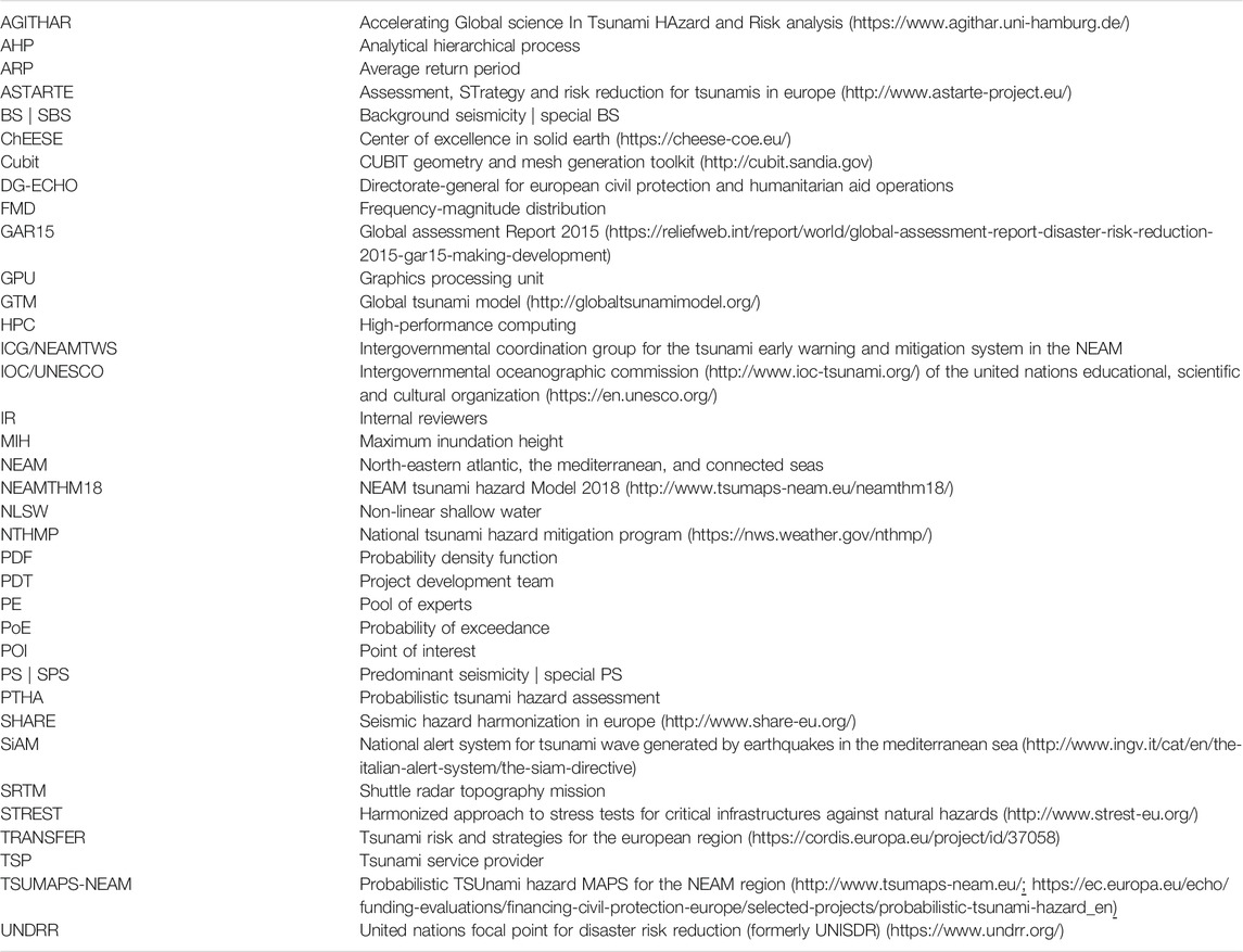
TABLE 1. List of Acronyms, abbreviations, and relevant websites.

The ICG/NEAMTWS was established in response to the Indian Ocean tsunami of December 26, 2004. NEAMTWS operates under IOC/UNESCO’s umbrella and is currently based on five national monitoring centers in France, Greece, Italy, Portugal, and Turkey that act as TSPs. Other ICGs support the development and maintenance of TWS in other oceans of the world (Figure 1). Tsunami risk assessment and warning systems need PTHA as input and reference to achieve effective risk reduction (IOC, 2017). Before 2004, it was already well-known that several destructive tsunamis had occurred in the NEAM region, such as the tsunamis caused by the caldera collapse in the Santorini Island in the Minoan Era, the Mw∼8 Crete earthquake in 365 CE and the Lisbon earthquake in 1755, and the Mw∼7 Messina and Reggio Calabria earthquake in 1908 whose associated tsunami was possibly enhanced by a seismically-induced submarine landslide (Maramai et al., 2014; Papadopoulos et al., 2014). Some of these events are among the most destructive tsunamis in history. Nonetheless, hazard analysis efforts for the NEAM Region started being pursued only in the wake of the 2004 disaster in the Indian Ocean. Often, they are high-resolution studies focusing on specific sub-domains (Tinti et al., 2005; Papadopoulos et al., 2010; Tonini et al., 2011; Álvarez-Gómez et al., 2011; Grezio et al., 2012; Sørensen et al., 2012; Omira et al., 2015), or are included in global assessments with a relatively limited spatial resolution (Løvholt et al., 2012; Løvholt et al., 2015; Davies et al., 2018). Others are methodological analyses that considered case studies in the NEAM Region (Grezio et al., 2010; Grezio et al., 2015; Lorito et al., 2015; Selva et al., 2016).

FIGURE 1

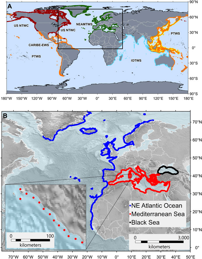
FIGURE 1. (A) ICGs global area of coverage map of TWS (IOC, 2015). The black rectangle shows the location of the map in the lower panel covering a large part of the NEAMTWS (Table 1). US NTWC, US national tsunami warning center (brownish red); IOTWS, indian ocean tsunami warning and mitigation system (turquoise); PTWC, pacific tsunami warning center (orange); CARIBE-EWS: interim of PTWC and US NTWC; PTWS: Northwest Pacific Tsunami Advisory Center/Japan Meteorological Agency (yellow), PTWC, and US NTWC. (B) Distribution of the Points of Interest (POIs) where the NEAMTHM18 hazard is calculated. The inset shows a close-up view of the POIs to appreciate their spacing and offshore location. Topo-bathymetry is from the ETOPO1 Global Relief Model (NOAA, 2009; Amante and Eakins, 2009).

During 2016 and 2017, the EU project TSUMAPS-NEAM developed the first long-term PTHA from earthquake-induced tsunamis for the NEAM Region (Figure 1), and in 2018 released the NEAM Tsunami Hazard Model 2018 (NEAMTHM18) (Basili et al., 2018). A large community of scientists and decision-makers were actively involved. The effort was funded by the EU DG-ECHO and formally supported by several potential end-users. TSUMAPS-NEAM built its strategy upon previous and ongoing projects, such as the EU projects ASTARTE and SHARE, the UNDRR GAR15, and national projects or initiatives supporting PTHA efforts like the NTHMP (United States) and SiAM (Italy) (Table 1). TSUMAPS-NEAM also considered the PTHA effort to promote an informed process of outreach, the definition of guidelines, and capacity-building initiatives for Europe and neighboring countries under the auspices of the DG-ECHO. Such actions could also strengthen the connection between TSPs, Civil Protection Authorities, and other national authorities, thereby reinforcing the NEAMTWS effectiveness, including awareness-raising actions for improving tsunami risk perception (e.g., Cerase et al., 2019). The PTHA at the entire NEAM Region scale is also meant to become a baseline for PTHA efforts toward a consistent approach to risk assessment and long-term risk mitigation and planning at national and regional levels. Therefore, the PTHA devised by TSUMAPS-NEAM relied on a shared understanding of the best viable practices and sought compliance with European scientific and policy standards for hazard and risk assessment. The NEAMTHM18 has already been taken as the reference model by Civil Protection Authorities in Italy (DCDPC, 2018). In analogy with the well-established practice for defining seismic building codes, a homogeneous hazard level from NEAMTHM18 was chosen to define the inundation zone. The definition of evacuation zones and long-term coastal planning are both based on these inundation zones. Similar approaches are being followed in New Zealand (MCDEM, 2016) and the United States (American Society of Civil Engineers, 2017), based on the local PTHA. The region-wide NEAMTHM18 is also being taken as a reference for higher-resolution site-specific PTHAs (Gibbons et al., 2020) and applications dealing with critical infrastructures at risk (e.g., Argyroudis et al., 2020). The development of standardized PTHA products (hazard curves, hazard and probability maps, exhaustive and transparent documentation, web tools for dissemination and analysis) is the first step to include tsunamis in multi-hazard risk assessment and mitigation.

In this paper, we describe the NEAMTHM18 as the main result of the TSUMAPS-NEAM project. NEAMTHM18 is a Poissonian time-independent hazard model dealing with tsunamis generated by earthquakes. The primary hazard intensity measure is MIH (Glimsdal et al., 2019). The hazard results are provided by hazard curves, calculated at 2,343 POIs distributed at an average spacing of ∼20 km along the NEAM coastlines, expressing the PoE in 50 years for different MIH thresholds.

The main challenges faced in the making of NEAMTHM18 were related to the diversity of tectonic environments hosting the potential seismic sources, the interconnections of large and small basins typical of the NEAM Region, the necessity to treat both near and distant seismic sources appropriately, and the vastness of the tsunami propagation domain requiring an intensive computational effort.

The hazard projects mentioned earlier undertook innovative approaches, followed by those specifically developed and implemented within TSUMAPS-NEAM. The first is the inclusion of sufficiently constrained 3D geometries for seismic sources (Selva et al., 2016; Tonini et al., 2020). The second is the potential of shallow slip amplification, as observed in recent tsunamigenic earthquakes (Romano et al., 2015a; Romano et al., 2020; Lorito et al., 2016) schematized as the effect of depth-dependent coupling and rigidity (Murphy et al., 2016; Murphy et al., 2018; Herrero and Murphy, 2018; Scala et al., 2019; Scala et al., 2020; Murphy and Herrero, 2020). The third is the massive use of HPC simulations with the multi-GPU Tsunami-HySEA benchmarked code (de la Asunción et al., 2013; Macías et al., 2017). The fourth is the approach to the tsunami reconstruction from precalculated elementary sources (Molinari et al., 2016), combined into the uncertainty propagation within a stochastic approach to inundation modeling (Glimsdal et al., 2019). Finally, the fifth is the quantification of uncertainty, combining ensemble modeling (Selva et al., 2016) with a multi-expert protocol for the management of subjective choices.

This paper provides a comprehensive overview of data, methods, and procedures adopted throughout the making of NEAMTHM18. It also illustrates the main results and discusses the model’s implications, limitations, and possible future developments. More details about the NEAMTHM18 can be found in the TSUMAPS-NEAM project website, which provides access to the model-specific documentation, from now on referred to as NEAMTHM18 Documentation (Basili et al., 2019), and also allows for navigating the NEAMTHM18 in a web mapper, consult hazard curves, and download model data.

Methodology and Data

NEAMTHM18 was designed as a three-phase project (Figure 2; Supplementary Data Sheet S1.1) involving three main teams: PDT, PE, and IR. The PDT interacted with the PE and the IR during the first two phases of the project. The interactions between the PDT and the PE followed the prescriptions of a formalized decision-making process based on a multiple-expert protocol. This protocol, which was inspired by similar protocols developed for seismic hazard (USNRC, 1997; USNRC, 2012; USNRC, 2018), was developed and applied in the EU project STREST (2013–2016) (Argyroudis et al., 2020; Esposito et al., 2020), and subsequently adapted to the TSUMAPS-NEAM project needs. The TSUMAPS-NEAM implementation of the protocol included two elicitation experiments of the PE to identify the model alternatives to be implemented and assign proper weights to the selected alternatives (Figure 2). Managing the subjectivity of choosing among alternatives in a structured way is necessary because a hazard model is never completely constrained by observations, nor is the physics of the hazardous phenomenon totally understood. Different scientifically acceptable alternative models and relevant datasets may thus be used, thereby reflecting the inherent uncertainty. The different alternative models may have different degrees of credibility within the reference scientific community. In principle, the model credibility should coincide with the accuracy of its output, but this is not always quantifiable because of the general lack of independent data for rare phenomena such as tsunamis. The basis of the conceptual elicitation model and its implementation are presented in detail in Selva et al. (2015) and the NEAMTHM18 Documentation (Basili et al., 2019). The interaction between the PDT and the IR took place in two review rounds, leading to extensive project documentation, which was initially shared only with the IR and made publicly available through the project website after incorporating the IR’s feedback.

FIGURE 2

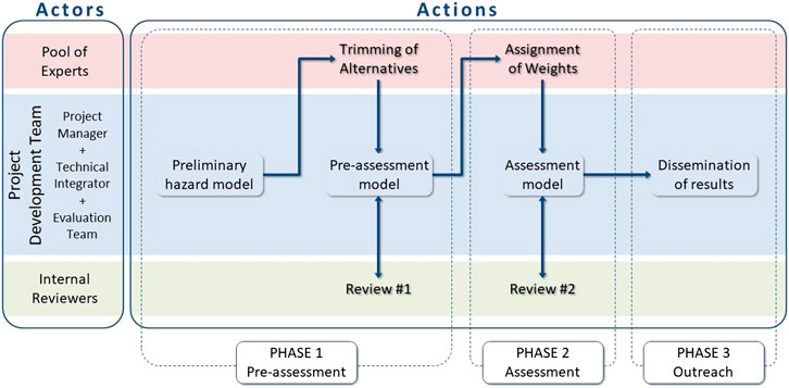
FIGURE 2. Schematic illustration of the project’s actors and correlative actions subdivided into three PHASES (Supplementary Data Sheet S1.1). Notice that both phase 1 and phase 2 include an elicitation experiment and a revision stage each. PHASE 3 includes the NEAMTHM18 Documentation (Basili et al., 2019) of the two preceding PHASES, a web mapper to access the main results of the hazard assessment, scientific publications, and some materials for illustrating the results to the general public (e.g., Layman’s Report).

The hazard assessment workflow is structured in “Steps” and “Levels” (Figure 3A), and the flux of information among the Steps proceeds along the paths illustrated in Figure 3B. There are four Steps, and each of them includes three to four Levels. Level-0 is common to all Steps and contains the definition of the used datasets. The other Levels constitute the finer grain of the hazard analysis within each Step, inside which the variables are treated as aleatory (for the aleatory variables in Step-1, see Supplementary Figure S1 for a detailed scheme). At each Level within each Step, several alternative approaches, datasets, and models are implemented to explore the epistemic uncertainty. A relatively high number of alternatives was initially presented to the PE. The first elicitation experiment, held during phase 1 (pre-assessment), served to select only the alternative models deemed to be the most important uncertainty drivers (Supplementary Table S1). The second elicitation experiment, held during phase 2 (assessment), served to establish the ranking of these alternatives by assigning weights to them (Supplementary Table S2). Below we first introduce the Steps and Levels and then summarize their rankings according to the second elicitation experiment results. Ensemble modeling for hazard aggregation and model uncertainty quantification will be presented in the description of Step-4. Further details on the implemented alternative models describing their epistemic uncertainty, selection, and weighing procedure using the elicitation experiments are given in the NEAMTHM18 Documentation (Basili et al., 2019).

FIGURE 3

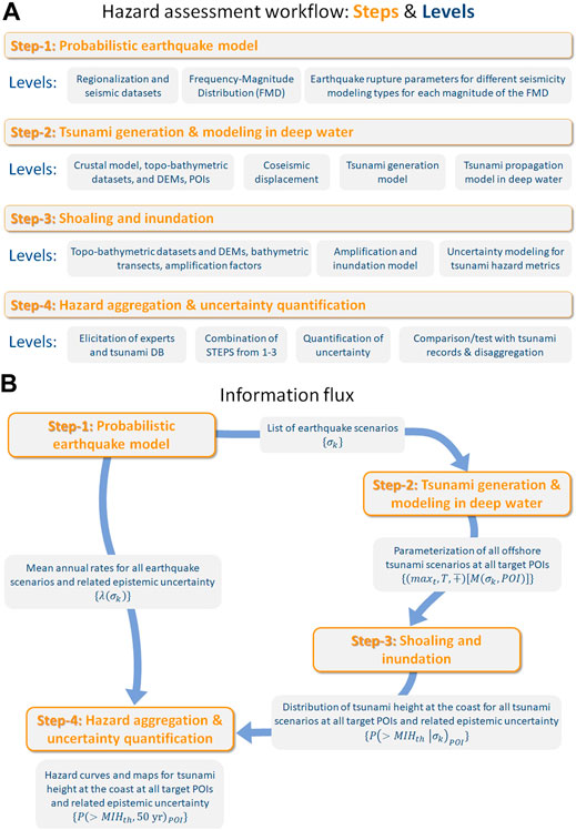
FIGURE 3. (A) Sketch of the NEAMTHM18 workflow. (B) Sketch of the information flux to build the hazard model. This procedure is repeated for each considered alternative model.

Step-1 concerns the Probabilistic Earthquake Model. It provides scenarios of all potential earthquakes in all considered seismic source regions, denoted as $\left\{{\sigma }_k\right\}$, and their mean annual rates $\left\{\lambda \left({\sigma }_k\right)\right\}$, according to their FMDs and the scenario parameters (earthquake magnitude, fault rupture position, strike, dip, rake, rupture size, and rupture slip). It also provides alternative modeling schemes of the above scenarios and their mean annual rates.

Step-2 concerns the Tsunami Generation and Modeling in Deepwater. It provides the deterministic numerical simulations of the seafloor displacement fields corresponding to the earthquake scenarios defined at Step-1. It also provides the deterministic numerical simulations of the tsunami generation from these seafloor displacement fields and their propagation from the source to each offshore POI, resulting in synthetic mareograms, defined as $\left[M({\sigma }_k,POI)\right]$, and parametric lookup tables of maxima (${\max }_t$), periods ($T$), and polarities ($\mp$) for all mareograms, defined as $\left\{\left[{\max }_t,T, \mp \right]\left[M({\sigma }_k,POI)\right]\right\}$.

Step-3 concerns Shoaling and Inundation. It provides both stochastic and deterministic models of the tsunami impact at all POIs defined in Step-2 for all the scenarios defined in Step-1. The tsunami generated by each seismic scenario is expressed by two metrics: the probability distribution for the MIH calculated by applying local amplification factor to the offshore results, such as $AF(T, \mp , POI)$, and the single-valued impact obtained through the application of Green’s law. Step-3 also provides the assessment of the alongshore tsunami variability as conditional hazard curves of the PoE of an MIH threshold value (MIH_th), denoted as $P{(>MI{H}_{th}|{\sigma }_k)}_{POI}$, and the assessment of the associated uncertainties, including those originating from linear combinations at Step-2.

Step-4 concerns the Hazard Aggregation and Uncertainty Quantification. It provides the probabilistic hazard model of the tsunami impact on NEAM coastlines expressed as the PoE in 50 years for different MIH thresholds $\left[P{\left(>MI{H}_{th},50\text{ yr}\right)}_{POI}\right]$. The model is obtained by aggregating all annual scenario rates from Step-1 with the conditional PoE from Step-3. The model uncertainties are expressed through distributions of hazard curves of the PoE and their statistics. It also provides the preparation and display of hazard and probability maps, disaggregation products, sanity checks, and other by-products presented in the NEAMTHM18 Documentation (Basili et al., 2019).

Step-1: Probabilistic Earthquake Model

The basic principle applied here is that knowledge of the potential earthquake sources is always limited, and we then acknowledge that earthquakes are possible everywhere. The level of knowledge of some seismic sources can be higher than for others (e.g., Basili et al., 2013b). It is advisable to deal with this heterogeneous uncertainty while maximizing the use of all the available information. We thus subdivided the seismicity into different modeling types, each adopting a different approach for one or more parameters, depending on the level of knowledge of the underlying data (Field et al., 2014; Woessner et al., 2015; Selva et al., 2016).

The seismicity modeling types are defined by the different modeling and parameterization approaches. Our approach depends on how well the various parameters are constrained relative to each other for any given seismic source in its context. To apply this concept, we defined two main seismicity types: predominant seismicity (PS) and background seismicity (BS) (Selva et al., 2016). The PS type captures the larger earthquakes generated by well-known major faults, such as plate boundaries and subduction interfaces. This approach to tsunamigenic seismicity is common in PTHA (e.g., González et al., 2009; Power et al., 2013), rooted in the assumption that relatively large earthquakes on known major faults dominate the tsunami hazard. Seismic sources of the PS type are then characterized by variability limited by the existing knowledge about them (e.g., fault geometry). The BS type captures all the diffuse seismicity in a tectonically-defined region. Therefore, sources of the BS type are characterized by the largest variability because of their lower level of knowledge, especially at the lower end of the earthquake magnitude values of interest. The BS type is less constrained by existing data and resembles seismic sources commonly adopted for seismic hazard analysis (Cornell, 1968), which have already been applied to tsunami hazard analysis (Sørensen et al., 2012). The above seismicity types may be modified to deal with specific situations considering the distance between the seismic source and the closest target coasts. In this respect, we defined two additional types: special PS (SPS) and special BS (SBS). While PS and BS types are two “end-members” featuring the maximum and the minimum number of fixed parameters, respectively, SBS and SPS types are intermediate cases in which the number of fixed and variable parameters is modulated case by case, also considering the necessary computational resources. These special cases are exclusive alternatives to each other and to the PS type, meaning that they are never considered together in the same source region.

Level-0: Input Data

Level-0 deals with the main input data that are used to build the probabilistic earthquake model. During phase 1 of the project (Figure 2), the possible alternatives to these input datasets were initially collected and analyzed. These potential alternatives were then reduced after the results of the elicitation experiment. Here we describe only the datasets retained for the actual hazard model implementation.

Tectonic Regionalization

The tectonic regionalization is a subdivision of the entire domain of potential seismic sources into discrete regions internally as homogeneous as possible based on the dominant tectonic processes. The adopted regionalization (Figure 4A) was built following basic plate tectonics principles and by refining or adapting the regionalization of the European seismic hazard model (Delavaud et al., 2012; Woessner et al., 2015). This regionalization is only a two-dimensional subdivision of the crustal volume. In subduction zones, one must consider the three-dimensional geometry of slabs.

FIGURE 4

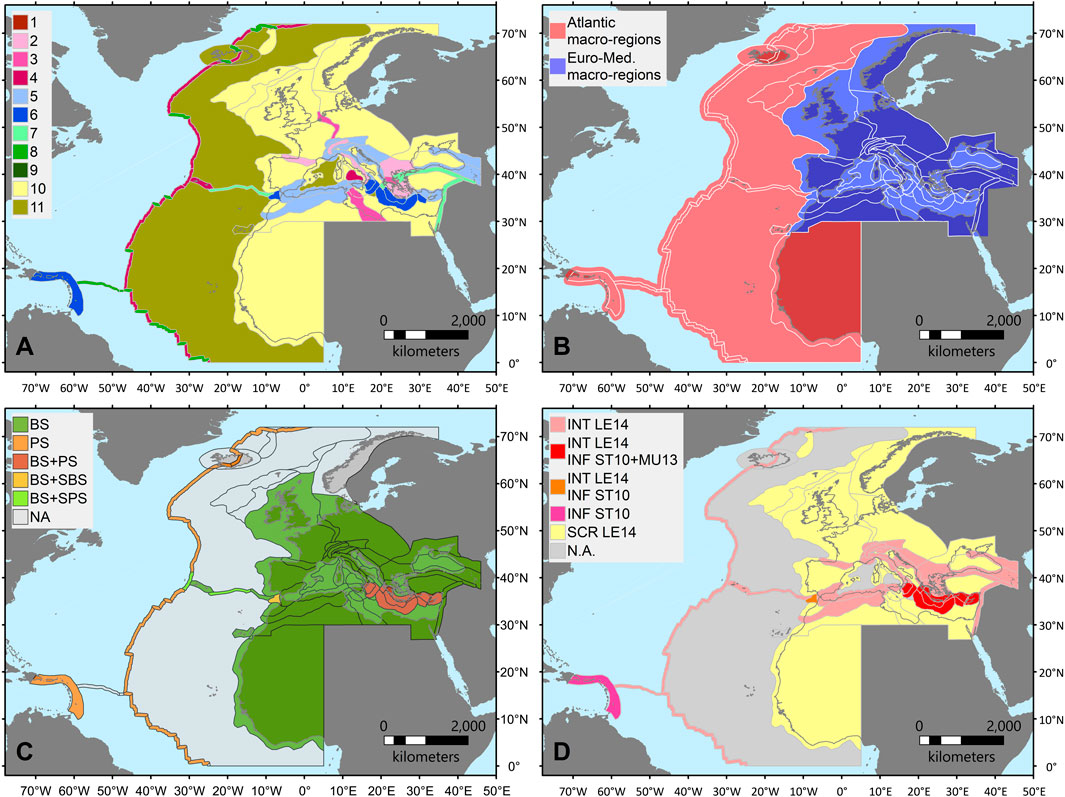
FIGURE 4. (A) Map of the regions, color-coded depending on the tectonic setting and dominant deformation style, covering the whole source area. 1) Active volcano; 2) Back-arc and orogenic collapse; 3) Continental rift; 4) Oceanic rift; 5) Contractional wedge; 6) Accretionary wedge; 7) Conservative plate boundary (mainly major transcurrent faults); 8) Transform fault s.s.; 9) Shield; 10) Stable continental region; 11) Stable oceanic region. (B) Map showing the macro-regions used to analyze the completeness of the adopted earthquake catalogs (Supplementary Figure S2). (C) Map showing the distribution of the seismicity model types assigned to each region of the tectonic regionalization. BS, background seismicity; PS, predominant seismicity; SPS, special PS; SBS, special BS; NA, not applied. (D) Map distribution of the adopted rupture scaling relations in the different tectonic settings. INT, interplate, crustal earthquakes; SCR, stable continental region, crustal earthquakes; INF, subduction interface. LE14 (Leonard, 2014); ST10 (Strasser et al., 2010); MU13 (Murotani et al., 2013); N.A, Not Applied.

Seismic Datasets

The seismic datasets are used to determine the rates of seismicity. To this end, earthquake catalogs need to geographically cover all the potential seismic sources during the longest possible time and be as homogeneous as possible in terms of parameterization. We thus employed two different datasets: 1) the ISC catalog (ISC, 2016) for the area within the Atlantic Ocean (period 1900–2015) and the SHEEC-EMEC catalog (Grünthal and Wahlström, 2012; Stucchi et al., 2013) for the Mediterranean region (period 1000–2006). Their respective areas of application are shown in Figure 4B, which were produced by merging regions from the tectonic regionalization (Figure 4A) into four macro-regions in the Atlantic Ocean and six macro-regions in the Euro-Mediterranean area. For these two earthquake catalogs, we performed statistical completeness analyses (Wiemer, 2001; Woessner and Wiemer, 2005) separately for each macro-region (Supplementary Table S3) and adopted the Gardner and Knopoff (1974) method for the declustering (Supplementary Figure S2). The non-declustered catalog is used to quantify annual earthquake rates and most other cases. The declustered catalog is used only to quantify the spatial distribution of BS-type sources through smoothed-seismicity (Level-2b).

Fault Datasets

The fault datasets aim to determine the orientation and sense of movement of future earthquake ruptures and, for a selection of them, the activity rate. To this end, we compiled two different datasets: focal mechanisms and geological faults. As with the earthquake catalogs, we favored geographic coverage over detail.

Regarding focal mechanisms, we considered the same macro-regions of the earthquake catalogs (Figure 4B). We adopted the global centroid moment tensors (Dziewonski et al., 1981; Ekström et al., 2012) for the North-East Atlantic and the regional centroid moment tensors (Pondrelli and Salimbeni, 2015) for the Euro-Mediterranean region (Supplementary Figure S3).

Regarding the geological faults, we retrieved data from large public fault databases, plus some original additions or revisions of specific cases (Figure 5). In this collection, we separated crustal faults from subduction systems. For crustal faults, we considered faults deemed capable of generating earthquakes of magnitude ≥5.5 both inland and offshore. For subduction systems, we considered three subduction interfaces in the Mediterranean Sea (Calabrian Arc, Hellenic Arc, Cyprus Arc) and two in the western Atlantic Sea (Gibraltar Arc and Caribbean Arc). Additional information about the Gloria fault and the Gibraltar Arc was derived from the ASTARTE project, deliverables D3.16 and D3.40. The rate of activity of a selection of these faults is based on the tectonic parameters (Supplementary Table S4) derived from Christophersen et al. (2015) and Davies et al. (2018). It is worth noting, though, that the rates and coupling coefficients in the three Mediterranean subduction zones are highly debated and variable (Laigle et al., 2004; Ganas and Parsons, 2009; Tiberti et al., 2014; Vernant et al., 2014; Carafa et al., 2018; Nijholt et al., 2018).

FIGURE 5

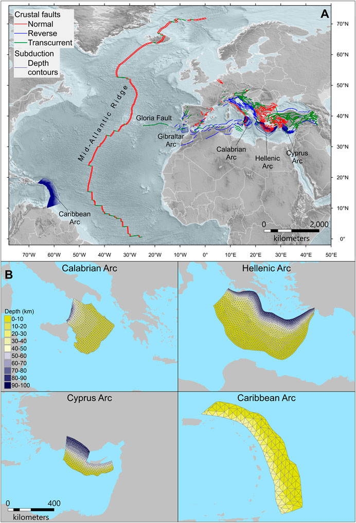
FIGURE 5. (A) Map of the fault datasets. The primary sources of information for the fault geometry and kinematics are as follows: the European database of Seismogenic Faults (EDSF) (Basili et al., 2013a; Woessner et al., 2015); the database of Individual Seismogenic Sources, DISS version 3.2.1 (DISS Working Group, 2018), used to replace EDSF in the central Mediterranean; the global plate boundary model (Bird, 2003) as a reference for the Mid-Atlantic Ridge and the Gloria fault. All crustal faults are color-coded based on their mechanism. The geometry of the three Mediterranean slabs was initially derived from the European database of Seismogenic Faults (EDSF) (Basili et al., 2013a; Woessner et al., 2015) and then modified according to newer data where available. In particular, the Calabrian Arc was entirely replaced by a recent model (Maesano et al., 2017) derived from the interpretation of a dense network of seismic reflection profiles integrated with the analysis of the seismicity distribution at depth. The Hellenic Arc is the same as that in EDSF, but we verified its consistency with recent works (Sodoudi et al., 2015; Sachpazi et al., 2016). The Cyprus Arc was slightly modified in consideration of results from recent works (Bakırcı et al., 2012; Salaün et al., 2012; Sellier et al., 2013a; Sellier et al., 2013b; Howell et al., 2017) that are based on seismic reflection profiles and tomographic and seismological data and constrain the geometry of the western part of the slab. The geometry of the Caribbean slab was entirely derived from an early version of the Slab two model (Hayes et al., 2018), provided as a courtesy by G. Hayes. All slab geometries are represented with depth contours, except for the Gibraltar Arc, which is represented by a sketch to show its location only. Topo-bathymetry is from the ETOPO1 Global Relief Model (NOAA, 2009; Amante and Eakins, 2009). (B) Map views of the meshes used to discretize the subduction interfaces with color-coded depths. The locations of these slabs are shown in panel (A). The meshes are built with element size set at ∼15 km for the three subduction interfaces in the Mediterranean Sea, and ∼50 km for the subduction interface of the Caribbean Arc, using the Cubit mesh generator (Casarotti et al., 2008). For all subduction interfaces, strike and dip are imposed by the discretization. Pure thrust faulting mechanism (rake 90°) is assumed for the Cyprus Arc because of the relatively small variability of the direction of plate convergence roughly normal to strike (Reilinger et al., 2006; Wdowinski et al., 2006), and the Caribbean Arc, according to other PSHA studies (e.g., Bozzoni et al., 2011). Variable rakes are used for the Calabrian Arc and Hellenic Arc in agreement with the direction of plate convergence.

Assignment of Seismicity Modeling Types to Different Seismic Sources

The four seismicity modeling types (BS, PS, SPS, SBS) are assigned to the regions resulting from the tectonic regionalization (Figure 4A) and are linked to relevant tectonic structures (Figure 4C). A maximum of two seismicity modeling types occurs in each region because the special cases (SPS and SBS) are alternative one to another. Faults shown in Figure 5A are geographically related to the regions of Figure 4A in this assignment.

The PS type is used in the Mediterranean area for the subduction interfaces of the Calabrian Arc, Hellenic Arc, and Cyprus Arc, and in the Atlantic area for the subduction interface of the Caribbean Arc and the crustal faults of the Mid-Atlantic Ridge far away from the Azores Islands (Figure 5A). The BS type is used everywhere in the Mediterranean area (Figure 4C), including regions overlaying the subduction interfaces (Figure 5A). In the Atlantic Ocean, the BS type is used for seismic sources near most coastlines (Figure 4C) but is neglected for seismic sources distant enough from some coastlines. One exception is the region around Iceland, where only PS is used. Possible seismic sources in the stable oceanic regions (Figure 4A) are ignored because seismicity rates seem to be too low to significantly contribute to tsunami hazards, according to global rates in this tectonic domain (Kagan et al., 2010). The SPS type is used for the Gloria Fault and a portion of the Mid-Atlantic Ridge near the Azores Islands (Figure 5A). SPS coexists with BS in all cases. The SBS type is used in the Gulf of Cadiz to model the Gibraltar Arc subduction interface (Gutscher et al., 2002; Duarte et al., 2013; Civiero et al., 2020), where the available geometric model (ASTARTE project deliverable D3.16) is a rather crude planar approximation. These choices are mainly due to the lack of computational resources to calculate elementary tsunami sources (Step-2), and therefore could change in future updates of the model.

Rupture Scaling Relations

Rupture scaling relations are used to determine the size of the earthquake ruptures and the geometrical discretization of the seismic sources. We initially reviewed the literature on fault scaling relations, analyzed the differences of their predictions, and tested their applicability to our modeling scheme. We adopted the scaling relations from Strasser et al. (2010) and Murotani et al. (2013) for the subduction interface earthquakes and those by Leonard (2014) for all crustal earthquakes. Although each scaling relation is subject to statistical uncertainty, we use only parameters from the best-fitting relations. Figure 4D shows the geographic distribution of their application in different tectonic regions.

Magnitude Discretization and Range

To improve the characterization of the FMD at higher magnitudes, we adopted a magnitude sampling that (roughly) becomes roughly exponentially finer as earthquake magnitude increases (Supplementary Table S5). This approach should allow for a more even sampling of the corresponding increase of the tsunami height, which seems nearly linear (Geist, 2012). The overall range of magnitude values modeled for each seismic source depends on different factors, such as fault size and discretization, seismogenic depth interval for subduction interfaces, crustal thickness, rupture scaling relations, and the distance between the seismic source and the target coastline. We adopted a lower threshold of Mw = 6 for seismic sources of seismicity model types (PS, BS, SBS, and SPS), except for seismic sources located far away from all target coastlines and modeled as PS type only, in which case we adopted a threshold of Mw = 7.3. The rationale for these limits is based on the FMD of globally analogous regions (Kagan et al., 2010). As not all possible earthquake magnitudes could be modeled, we tested the impact of unmodeled earthquakes at both ends of the considered magnitude range onto the hazard. The results of these tests are reported in the NEAMTHM18 Documentation (Basili et al., 2019).

Discretization and Parameterization of the Seismic Sources

A 3D geometry characterizes the subduction interfaces treated as PS type. Although 3D reconstructions yield more accurate representations of earthquake ruptures (Tonini et al., 2020), they are not available everywhere. Where available, their discretization must reflect the resolution of the data and constraints imposed by the modeling strategy. Starting from the slab geometries, we built 3D meshes (Figure 5B) with triangular elementary sources (subfaults) for setting the coseismic slip, which determines the seafloor displacement applied as a tsunami initial condition. The size of subfaults constrains the minimum modeled earthquake magnitude, considering the adopted scaling relations and the allowed maximum wave numbers of the slip spatial distribution. The crustal faults treated as PS types are the transcurrent (transform) and normal faults of the Mid-Atlantic Ridge and the Gloria Fault. They were discretized into rectangular subfaults (Figure 6A). As subfaults must be combined to form individual ruptures for different magnitudes, their size was determined to minimize deviations from the adopted scaling relations. Details of these parameters are provided in Supplementary Table S6. A summary of the implemented earthquake magnitude and depth ranges for all seismic sources modeled as PS type is provided in Supplementary Tables S7, S8.

FIGURE 6

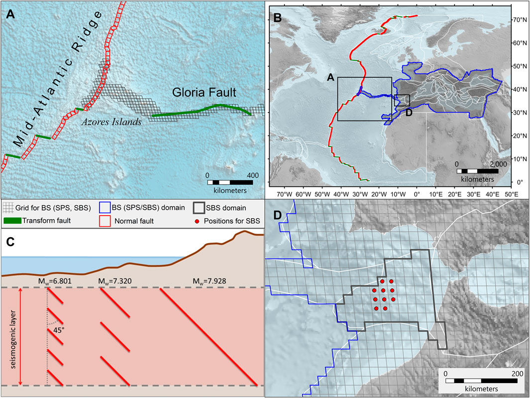
FIGURE 6. (A) Close-up view of the Predominant Seismicity modeling type (PS) discretization in subfaults of the Mid-Atlantic Ridge and the Gloria Fault near the Azores Islands. Location of this map in panel (A). There are in total 270 rectangular subfaults; 214 normal faults with a constant dip angle of 45° and size of 40 × 45 km; 57 strike-slip (transform) faults with a constant dip angle of 90° and size of 55 × 20 km. See Supplementary Table S6 for the combinations of subfaults to make up large ruptures. The grid for the BS and SPS in this zone is also shown. (B) Regular grid (grey quadrangles, see the zoomed-in inset) composed of non-conformal equal-area cells of 25 × 25 km with the origin at 24°N–3°E for the discretization of the background seismicity modeling type (BS). Note that cell sides depart from right angles with increasing distance from the origin in this projection. The red outline marks the calculation domain, outside which only the predominant seismicity modeling type (PS) is modeled. The white outline of the tectonic regionalization (Figure 4A) is shown for reference. (C) Schematic of depth discretization for BS and SPS types due to the magnitude of earthquake ruptures applied to the center of each cell of the grid. For the SBS type, the magnitude range is extended to Mw = 9.026, and the depth limit of the crustal model is ignored. All magnitudes are always modeled for the shallowest depth position, irrespective of the crustal thickness being exceeded or not. Where the crust is very thin, some of the deeper positions are not occupied if the rupture crosses the base of the crust. (D) Cells of the grid (spatial discretization) in the Cadiz region showing the positions (center of 10 grid cells) occupied by the SBS type of the Gibraltar Arc subduction interface. Location of this map in panel (A). Topo-bathymetry is from the ETOPO1 Global Relief Model (NOAA, 2009; Amante and Eakins, 2009).

The domain of the BS and SBS types is uniformly discretized into a grid (Figure 6B) trimmed where seismic sources are close to the target coastlines. At each grid cell, the earthquake ruptures can occur within the entire crustal thickness derived from the 1D global crustal model CRUST 1.0 (Laske et al., 2013) depending on the rupture width at the modeled earthquake magnitude (Figure 6C).

The rupture mechanisms may differ in each grid cell based on the available information from focal mechanisms and known faults. The discretization of the faulting mechanisms is made separately for each strike, dip, and rake by applying a reversible transformation (Selva and Marzocchi, 2004) from the standard convention (Aki and Richards, 1980). Considering four intervals for the strike, nine for the dip, and four for the rake yields 144 combinations. The Gibraltar Arc, modeled as SBS type, adopts a strategy like the BS type, but with more limited variability of rupture positions and faulting mechanism while allowing for larger magnitudes and depth range (Figure 6D).

Seismicity Separation in Catalogs

Once the regionalization is set (Figure 4) and all the tectonic sources are assigned to the four seismicity modeling types with their parameters defined, we need to separate the earthquakes assigned to individual faults of the PS/SPS from the earthquakes that remain within the BS/SBS. This separation is done by using two alternative cut-off distances of 5 km and 10 km. That is, assigning the seismicity within the cut-off distance to the PS and the remaining seismicity to the BS. We did not apply this procedure to the SBS (i.e., the Gibraltar Arc) because of its uncertainty in position and geometry. This hard-bound cut-off method is preferred over more sophisticated softer cut-offs (e.g., Bird and Kagan, 2004) because the Boolean separation provides two distinct catalogs of PS/SPS and BS/SBS events, which facilitates the implementation of the subsequent Levels.

Level-1: Frequency-Magnitude Distributions

The annual earthquake rates are based on the available seismicity data and tectonic data (convergence rates or slip rates) for selected PS as provided at Level-0. The earthquake rate determinations are also influenced by the assumption that larger earthquakes are increasingly likely to occur on major faults, possibly treated as PS/SBS/SPS types.

We implemented a set of Bayesian alternatives for quantifying the earthquake FMDs and their associated epistemic uncertainty, especially on annual rates and FMD tails. These alternatives concern the joint or separate quantification of earthquake rates for each seismic source, which allows for considering earthquake rate estimations derived from seismicity or tectonic rates, and functional forms (shape) of the FMDs and their parameters.

For the joint PS/BS quantification, the FMD is calculated in two stages (Selva et al., 2016; Taroni and Selva, 2020) first evaluating a global FMD distribution in each region and then separating this global FMD into PS/SPS/SBS and BS contributions, in regions where PS/SPS/SBS types are present. Both stages are based on a Bayesian formulation, with data coming from the non-declustered complete seismic catalog. This choice, also supported by the IR team, was made to avoid the significant underestimation of the real hazard that the declustering procedure may produce (Boyd, 2012; Iervolino et al., 2012; Marzocchi and Taroni, 2014). As shown by Kagan (2017), the Poisson distribution can also be used for non-declustered seismic catalogs if one is interested in modeling strong events (Mw > 6.5). Regarding the functional forms, we implemented both truncated and tapered Pareto formulations (Kagan, 2002a; Kagan, 2002b). Truncation and tapering are both applied to the probability density functions (PDFs). The parameters to be set are the rate for the smallest considered magnitude, the corner or the maximum magnitude (Mc or Mmax, for tapered and truncated distributions, respectively), and the scale parameter β (2/3 of the Gutenberg-Richter b-value). We set Mw = 5.0 as the minimum magnitude for assessing the rates, which is smaller than the minimum magnitude considered by the earthquake scenario (Supplementary Table S5) but allows for more robust rate estimations. The prior distributions are set as non-informative for the rates and the Mc (tapered Pareto). The Mmax for the truncated Pareto is set as discussed in Level-0, considering all known constraints (e.g., maximum magnitude observed in the region).

Two alternatives are implemented for estimating the parameter β. The first alternative is to compute the b-value from data by setting a weakly informative Gamma prior distribution centered on the worldwide tectonic analogs from Kagan et al. (2010) with variance corresponding to an equivalent sample size of 10. If there is a large dataset (>>10 samples), β is entirely controlled by the data, while in the case of very few data, the distribution is pushed toward the worldwide value. The second alternative is to force the b-value to be equal to one regardless of the observed seismicity in the region. As regards to the separation, we assumed a sigmoidal polynomial function that assigns a smooth transition between a high-magnitude regime where all earthquakes are supposed to be of PS/SPS/SBS type, a low-magnitude regime with a constant ratio between BS and PS/SPS/SBS, and an intermediate-magnitude regime where the ratio smoothly increases up to one (Figure 7A). Uncertainty on the three parameters of the separation (two magnitude thresholds separating high-, intermediate-, and low-magnitude regimes, and the ratio between BS and PS/SPS/SBS in the low-magnitude regime) is considered, with 1) uniform distribution for the lower threshold between magnitude five and six; 2) a uniform distribution for the higher threshold between magnitude six and seven in crustal BS and between magnitude seven and eight in subduction interfaces; and 3) a non-informative prior (uniform between 0 and 1) updated by likelihood functions based on the observed fraction between the PS/SPS and the BS earthquakes. Both alternative separation procedures are adopted, yielding two alternative separation models. These choices produce a total of 2 × 4 = 8 Bayesian alternative implementations for the joint PS-BS quantification of the FMD, with two alternative functional forms (tapered vs. truncated Pareto), two b-values (from data or set to 1), and two seismicity datasets from the two cut-off distances from PS. All of them are Bayesian alternatives; hence they automatically include the epistemic uncertainty emerging from parameter estimations. To propagate this uncertainty to the hazard results, we resampled these models 1,000 times, thereby providing 1,000 alternative realizations of the Bayesian model.

FIGURE 7

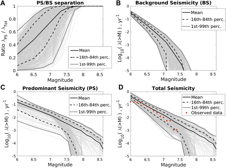
FIGURE 7. Example of frequency-magnitude distributions for the Kefalonia-Lefkada, Greece, region. (A) Ratio between seismicity assigned to the PS type and total seismicity, evaluated with the Bayesian separation model. (B) BS seismicity type computed for all the alternative models (1,000 samples) and statistics of the epistemic uncertainty. (C) Same as panel (B), but for PS seismicity. (D) Total seismicity, obtained by summing the BS and PS contributions, compared with the observed data from the relevant seismicity catalog. Grey lines in all panels represent the distribution samples.

Further alternative FMDs for PS are set from Christophersen et al. (2015) and Davies et al. (2018), starting from tectonic convergence or slip rates (Supplementary Table S4). Conversely, the FMD for BS could not be quantified with a similar strategy due to the lack of resources. Therefore, each FMD for PS is complemented by randomly sampling one FMD for BS from the two-stage PS/BS quantification. In this way, the two quantifications are independent since they are based on different input data.

To derive the FMDs for PS from tectonic data, we adopt two functional forms, the characteristic and the truncated Pareto (Kagan, 2002a; Kagan, 2002b) (Supplementary Table S2), considering three alternative maximum magnitudes, three alternative b-values, three alternative estimations for the seismic coupling (Supplementary Table S4), we obtain 3 × 3 × 3 × 2 = 54 alternatives.

In Figures 7B–D, we provide an example implementation in the Kefalonia-Lefkada region (Ionian Islands, Greece) of the four -BS/PS Bayesian FMDs models and the 54 models of BS/PS separated seismicity (separated into two groups, one for truncated Pareto and another for characteristic G-R). This region includes part of the Hellenic Arc, i.e., both PS and BS. The resulting modeled total FMDs (sum of BS and PS contributions) are compared with data. The results for the remaining four Bayesian models, relative to the 10 km-wide cut-off, are equivalent.

Level-2: Earthquake Rupture Variability

The variability of earthquake ruptures for PS/SPS types (Level-2a) is analyzed in terms of rupture position and area on the hosting structures and, importantly, slip distribution. The position and size of the rupture area are treated simultaneously. Earthquake positions on each hosting fault are discretized by defining a set of coordinate pairs representing the rupture center on the fault geometry. The assessment consists of quantifying the joint probability of a rupture center, a rupture area, and slip for an earthquake of a given magnitude in the region. Earthquake magnitude, rupture area, and slip are derived from rupture scaling relations without considering their uncertainty. For PS and SPS in the Atlantic region (distant seismic sources), we use only the rupture scaling relation of Strasser et al. (2010) for earthquakes in the Caribbean subduction and that of Leonard (2014) for crustal earthquakes (Figures 4C,D). For the Mediterranean PS subduction interfaces, we adopted the scaling relations from Strasser et al. (2010) and Murotani et al. (2013). Murotani et al. (2013) predict larger areas and smaller average slips at larger magnitudes than Strasser et al. (2010). These scaling relations provide only the average slip in the rupture area. Here, we also model the aleatory variability of the heterogeneous slip distribution for the larger earthquakes on the Mediterranean subduction interfaces because they are close to target areas (Figure 5). We use the classic k⁻² stochastic slip distributions on a non-planar surface, applying a technique that has been previously validated (Herrero and Murphy, 2018). Two alternative models have been considered: one considers depth-independent rigidity, the other considers shallow slip amplification controlled by depth-dependent rigidity variations (Bilek and Lay, 1999) while preventing systematic slip excess at shallow depths over one or more seismic cycles (Scala et al., 2020) (Supplementary Figure S4). For all the other structures assigned to PS and SPS, the slip is assumed to be uniform according to the average value resulting from the adopted scaling relation.

The earthquake ruptures variability of the BS/SBS types (Level-2b) is analyzed in terms of spatial distribution, depth distribution, and faulting mechanism. The variability associated with the rupture area and slip is not explored because only one rupture scaling relation is adopted for BS and SBS cases (Figures 4C,D). We use the smoothed seismicity approach (Frankel, 1995) to compute the spatial seismicity distribution and introduce a correction to account for the variability of the completeness magnitude in the spatial smoothing (Hiemer et al., 2014) to increase the number of seismic events considered. This approach enables longer intervals of the catalog, adopting an increasing magnitude of completeness while exploring older seismicity. The analysis is based on the complete part of the declustered catalog considering the two alternative cut-off distances (Figure 8).

FIGURE 8

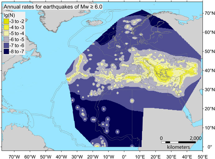
FIGURE 8. Map showing the geographic distribution of annual earthquake rates (common logarithm scale) for Mw ≥ 6.0 for the BS/SBS seismicity model types, adopting the cut-off distance of 5 km for the seismicity separation between PS and BS. This separation is done by assigning the earthquakes located within the given cut-off distance from the PS sources (Figures 4, 5) to the PS/SPS types and the remaining earthquakes to the BS/SBS types. The hazard model also includes the distribution of annual earthquake rates calculated with the cut-off distance of 10 km.

Regarding the focal depth, all possible depths of the discretization shown in Figure 6 are considered equally probable. In each cell of the spatial domain, various faulting mechanisms are possible for the modeled earthquake ruptures. The probabilities of these mechanisms are not uniform, and their expected PDF is derived through a Bayesian method according to centroid moment tensors of observed seismicity and data on known faults (Selva et al., 2016). The likelihood is modeled as a multinomial distribution based on the non-declustered entire (without considering completeness) catalogs of focal mechanism (Supplementary Figure S3), considering the two alternative cut-off distances (BS type only) and both nodal planes of each focal mechanism (Selva and Sandri, 2013). If faults occur in a grid cell, a Dirichlet distribution is set by forcing an average equal to the fault strike, dip, and rake of the fault fraction intersected by the cell, weighting this information ten times as much as that from the focal mechanisms. When multiple faults are present in one cell, their mechanisms are weighted by their respective moment rate. Figure 9 shows the geographic distribution of the resulting mechanisms classified as normal, reverse, and transcurrent. For simplicity, only the faulting mechanism with the highest probability (mode) is represented in each cell.

FIGURE 9

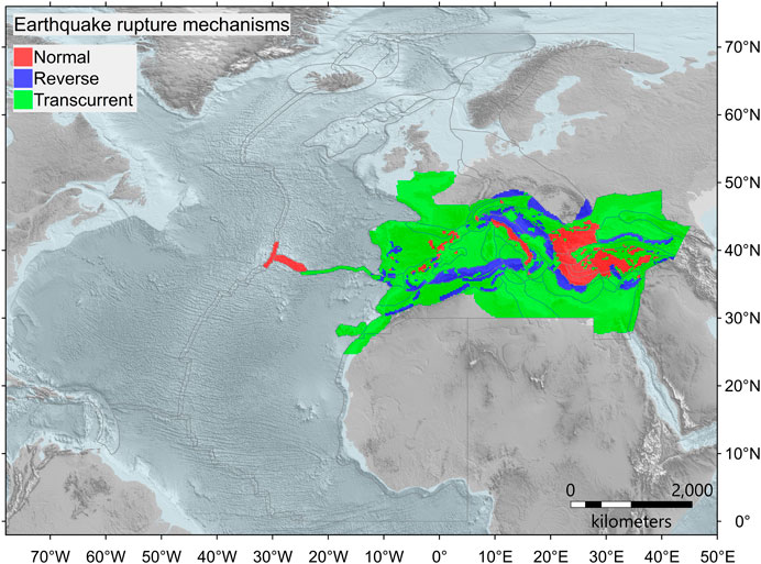
FIGURE 9. Geographic distribution of crustal earthquake rupture mechanisms within the calculation domain for the BS/SPS type. Only the most probable mechanism in each grid cell is shown for simplicity. The complete distribution consists of strike discretization at four intervals of 45° starting from 22.5° clockwise from North, and dip discretization at nine intervals of 20° within the 0°–180° range. The rake discretization is at four intervals of 90°, corresponding to normal, reverse, left-lateral strike-slip, and right-lateral strike-slip. Altogether, this makes a total of 4 × 9 × 4 = 144 combinations of the strike, dip, and rake values. For the SBS type (Figure 6D), the variability of the mechanism is limited to four combinations (strike of 22.5° and 337.5°; dip at 10° and 30°, and rake fixed at 90°). Topo-bathymetry is from the ETOPO1 Global Relief Model (NOAA, 2009; Amante and Eakins, 2009).

Step-2: Tsunami Generation and Modeling in Deepwater

In PTHA, it is common to use nonlinear shallow water (NLSW) models with wetting and drying to compute inundation and runup. As of today, NLSW simulations of coastal inundation are not yet affordable in the case of region-wide PTHA requiring millions of seismic scenarios. Moreover, sufficiently high-resolution bathymetry and topography models are not always available, which may discourage precise deterministic simulations. Conversely, simulations in deep waters may be conducted with reasonable accuracy by numerical integration of shallow water equations using relatively low-resolution bathymetric models available in the public domain. We thus separate tsunami modeling into two stages, one at Step-2 for generation and propagation in deep waters, and one at Step-3 for the coastal processes, characterized by larger uncertainty.

In Step-2, we assume linearity between the size of the tsunami and the coseismic displacement at the source. This approach makes Step-2 affordable from the computational viewpoint. Step-2 then provides the input to Step-3, which consists of synthetic tsunami mareograms and their parameters at offshore POIs.

Hence, Step-2 can be further divided into three main goals. The first is the deterministic numerical simulation of seafloor displacement corresponding to the individual earthquake scenarios defined at Step-1. The second is the deterministic numerical simulations of the tsunami generation and propagation from each source to any offshore POI. The third is the analysis of the mareograms to extract wave amplitude maxima, wave periods, and polarities for later use in Step-3.

Level-0: Input Data

The adopted crustal model for coseismic displacement calculations is an infinite half-space with the properties of an elastically homogeneous Poisson solid (e.g., Okada, 1992).

The topo-bathymetry model generally employed is SRTM30+ (Becker et al., 2009), which has a grid spacing of 30 arc seconds (∼900 m), improved with local data in the Gulf of Cadiz (Zitellini et al., 2009). In the Black Sea, SRTM15+ (Tozer et al., 2019) resampled to 30 arc seconds is used.

The POIs are the locus of tsunami simulation outputs, and subsequent tsunami hazard quantities are derived from the topo-bathymetric models around them. We set our POIs to nominally lie along the 50-m isobath with a spacing of roughly 20 km from each other (Figure 1). The POI depths have some variability related to the approximations made during the extraction of the 50 m-depth contour from the regularly gridded data with the GMT algorithms (Wessel et al., 2013) forced to remain within 40–100 m. The POIs outside this range are discarded. Hence, the distance between two adjacent POIs can be occasionally larger than 20 km, typically in areas with very steep slopes.

The spacing of POIs is a compromise between coastline coverage, computational cost, and storage containment. Similarly, the POI depth range is a compromise between preserving the linearity of the tsunami propagation and the need to be as close as possible to the target coastline. In principle, linearity should be guaranteed by ensuring the tsunami amplitude remains much smaller than the water depth. Linearity is needed to cope with the huge number (∼50 million) of seismic scenarios, coupled with the geographical scale of the investigated region through a linear superposition of pre-computed virtual POI tsunami time-series from elementary sources (Molinari et al., 2016).

It must be noted, though, that there are also locations where a POI cannot be realistically associated with the coast behind it because it is too distant. This circumstance occurs, for example, in the southern part of the North Sea, in the northern Adriatic Sea, and on the eastern coast of Tunisia. In all such cases, special care should be adopted if using the results at the local scale.

Level-1: Coseismic Displacement Model

Level-1 concerns the coseismic seafloor displacement for each earthquake scenario defined at Step-1. Each earthquake scenario corresponds to a single fault rupture characterized by a set of parameters, including location, geometry (fault size and orientation), and rake-parallel slip vector. The coseismic seafloor displacement is modeled using Volterra’s formulation of elastic dislocation theory applied to faults buried in an infinite elastic half-space. To this end, we used the analytical model by Okada (1992) in the case where fault ruptures consist of single or multiple planar quadrangles, and the code by Meade (2007) in the case of 3D triangular meshes, as defined in Step-1. Slip vectors are always constant for planar faults, whereas they can be either constant or variable for non-planar faults, as described in Step-1, Level-2a. The total seafloor deformation is computed as a linear superposition of contributions from the individual patches that describe the fault. The vertical component of the seafloor displacement, sampled on a regular 30 arc-second grid roughly centered automatically on the rupture, is used as input for Level-2, where the tsunami generation is treated. Since the fault elastic dislocation in an infinite elastic half-space solution produces very long “tails” of low-amplitude surface displacement, for practical reasons, we restricted the deformation area to vertical displacements larger than 1 cm.

Level-2: Tsunami Generation Model

Level-2 deals with the initial tsunami conditions at the surface derived from the seafloor vertical deformation obtained at Level-1. To account for the attenuation of the short wavelengths through the water column, we applied a two-dimensional filter of the form 1/cosh(kH) (Kajiura, 1963) to the static vertical seafloor deformation field calculated at Level-1. Here k is the wavenumber, and H is the effective water depth taken as the average above the fault. This filter is performed through forward and backward fast Fourier transforms with the high-pass filtering applied to the Fourier image in between. Because of the constant water depth requirement, this approach has a drawback in the case of large ruptures stretching over highly variable bathymetry. The Kajiura (1963) filtering was not applied to all sources treated as rectangular subfaults, including all the relatively shallow but mostly distant sources of the Gloria Fault, the Mid-Atlantic Ridge, and the Caribbean Arc.

Level-3: Tsunami Propagation Model in Deepwater

Level-3 concerns the simulation of tsunami mareograms at the offshore POIs (Figure 1), according to the initial conditions evaluated at Level-2 for all the considered earthquake scenarios. These offshore time-series are also further analyzed to derive the principal wave characteristics, such as the maximum amplitude, period, and polarity, that are necessary inputs for the subsequent processing at Step-3.

The mareograms are obtained as linear combinations of Green’s functions to save computational resources. The coefficients of the linear combinations (i.e., weights of the Green’s functions) reflect the initial displacement computed at the previous Levels in this Step. Two types of tsunami Green’s functions are used. The first is the type associated with Gaussian-shaped sea-level elevation unit sources. The second is the more usual type considering unit slip at elementary subfaults. This choice was made for practical reasons because the Gaussian tsunami database for the Mediterranean Sea already existed, and it was then extended farther to the Black Sea and part of the Atlantic Ocean. In some other cases, it was less expensive computationally to adopt the subfault approach, e.g., in the case of distant sources not requiring modeling of low earthquake magnitudes. More details are found in the NEAMTHM18 Documentation (Basili et al., 2019).

Green’s functions were simulated with the Tsunami-HySEA NLSW GPU-optimized code (de la Asunción et al., 2013). The code has been benchmarked at NTHMP benchmarking workshops (Lynett et al., 2017; Macías et al., 2017; Macías et al., 2020a, Macías et al., 2020b). The open boundary at the coast is used as boundary conditions. The spatial resolution of the simulation grid is 30 arc seconds. Tsunami-HySEA automatically adapts the time-step to match the Courant–Friedrichs–Lewy stability condition for the deepest point in the simulation grid. The simulated time was 4 h in the Black Sea, 8 h in the Mediterranean Sea, and up to 16 h in the Atlantic Ocean. More details are found in the NEAMTHM18 Documentation (Basili et al., 2019). Simple linear combinations according to local slip values were performed for the elementary tsunamis generated by the subfaults. Conversely, for the Gaussians, we use an algorithm for sea level displacement reconstruction and unit sources linear combination coefficient determination starting from an arbitrary fault (Molinari et al., 2016).

The last activity within Level-3 of Step-2 is the post-processing of the mareograms obtained via linear combinations. The post-processing phase is necessary to obtain the main wave characteristics needed for applying the amplification factors at Step-3. These are stored as matrices providing the amplitude, leading wave polarity, and dominant wave period at each POI for each considered scenario in the seismic model. The post-processing algorithm is described in the NEAMTHM18 Documentation (Basili et al., 2019) and in the study that deals with the local amplification factors and the uncertainty propagation procedure (Glimsdal et al., 2019).

Step-3: Shoaling and Inundation

Step-3 aims to evaluate the tsunami height at the coast, starting from the synthetic mareograms and their parameters computed offshore at each POI in Step-2. Our main metric to express tsunami size on the coast is the MIH measured relative to the mean sea level (Supplementary Figure S5) for the entire event duration.

Level-0: Input Data

As for Step-2, the SRTM15+ bathymetric model (Tozer et al., 2019), which has a grid spacing of 15 arc seconds (∼450 m), was used for extracting the profiles in the Mediterranean Sea and the Black Sea. For the North-East Atlantic, we used the SRTM30+ (Becker et al., 2009), which has a grid spacing of 30 arc seconds (∼900 m), improved with local data in the Gulf of Cadiz (Zitellini et al., 2009). The latter is the same already used in Step-2, Level-0.

This Level also provides 1D amplification factors that transform the incident wave amplitude into an MIH value based on local bathymetric profiles. The basic principles of the 1D method are described by Løvholt et al. (2012) and Løvholt et al. (2015). Here, we employ an improved version of this amplification method, which was partly developed within the ASTARTE project (deliverable D8.39) and then further developed and completed by Glimsdal et al. (2019). The latter describes how the amplification factors, which depend on the period and polarity of the incident wave and the local bathymetric profile, were calculated. For this, we used incident waves with leading peak (positive polarity) and leading trough (negative polarity), and wave periods of 120–3600 s. These amplification factors are provided as lookup tables providing the amplification factor value for each specific location as a function of the period and polarity.

The procedure to acquire the bathymetric profiles (Supplementary Figure S5) begins with extracting offshore POIs along a 50 m depth contour with an initial separation distance of ∼20 km. The nearest-neighbor algorithm is then used to identify the nearest coastal point. These designated coastline points, also separated by roughly 20 km, were then applied to define a piecewise linear shoreline contour. A set of 40 transects, spaced at about 1 km and perpendicular to this contour line, were then created (i.e., 20 km to each side of the onshore hazard points). All profiles that intersected islands were deleted to avoid positive values (i.e., land). Profiles with anomalous orientation relative to the shoreline in areas characterized by complex non-planar coastlines or regions with many islands (e.g., Aegean and Croatian islands), deep and narrow bays (e.g., fjords) were identified, and transect positions were drawn manually. Further details can be found in Glimsdal et al. (2019).

The approach developed by Glimsdal et al. (2019) also addresses stochastic inundation modeling to consider the 2D character of the inundation process and its uncertainties. It also allows for propagating the uncertainty stemming from the previous Steps. Another dataset is the relative error distribution related to the approximation of the deep-sea tsunami propagation as a linear combination, introduced at Step-2. This modeling uncertainty distribution is one of those provided by Molinari et al. (2016). Moreover, to quantify the epistemic uncertainty related to the simplification made with the 1D amplification factors, we compared the obtained MIHs with the results of local high-resolution 2D NLSW numerical inundation models in six test sites where high-resolution bathymetric and topographic models were available from the ASTARTE project. One site is in the Atlantic Ocean at Sines, Portugal, whereas the other five sites are in the Mediterranean Sea, at Colonia Sant Jordi, Mallorca Island and SE Iberia (Spain), Siracusa and Catania (Italy), and Heraklion (Greece). In this way, we obtained the distributions of the bias and the variability of the inundation. The details of the applied methodology and the obtained uncertainty distributions can be found in Glimsdal et al. (2019). We recall that the numerical simulations are done in the 2D vertically-averaged NLSW, which is still approximate. For example, 3D free-surface Navier-Stokes models would be, in principle, more accurate. However, numerical simulations cannot replace observations, and tsunami run-up data generally do not suffice for hazard calculation purposes.

Level-1: Amplification and Inundation Model

The local coastal tsunami impact is here expressed by one primary and one alternative hazard intensity metric. Our primary metric is the MIH. An alternative metric is obtained via amplification through Green’s law (e.g., Kamigaichi, 2011).

At this Level, the amplified MIH values corresponding to all the different tsunamis generated by the individual seismic sources at each POI are obtained by applying the lookup tables from Level-0 to the matrices of tsunami parameters provided by Step-2. Also, the simplest form of Green’s law is applied. This relation defines the ratio between the offshore value $H_D$ at a given depth $D$ and the amplified value $H_d$ after shoaling to a certain reference depth $d$, that is $H_d=H_D\sqrt[4]{D/d}$. We fix as customary this reference depth $d$ to 1 m. $D$ is the depth of the POIs. In this way, if a POI lies at a depth of 50 m, the amplification obtained via Green’s law is, for example, ∼2.66 times the maximum elevation provided by the mareogram.

Note that using Green’s law is not an alternative model. It estimates a different tsunami hazard intensity metric, not an alternative approach to estimating the same metric. However, this allowed us to define a sanity check on NEAMTHM18 results, comparing them with what we would have obtained adopting an alternative amplification scheme. These sanity check results are presented in the NEAMTHM18 Documentation (Basili et al., 2019). The application of MIH from the amplification factors and Green’s law does not require large computational efforts or very-high grid resolution for the offshore input simulations.

Level-2: Uncertainty Modeling

At Level-2, we quantify and sample the distributions describing the aleatory and epistemic uncertainty associated with tsunami modeling. The epistemic uncertainty related to the probability of exceeding a certain threshold MIH should account for the uncertainty inherent in the amplification factor method and uncertainties that may arise at the previous Steps due to different model approximations and non-modeled effects (Davies et al., 2018). These uncertainties are expressed with a conditional PoE, and the relative uncertainty is subsequently used at Step-4 combined with source probabilities for hazard assessment.

To start with, the probability of exceeding different values of threshold MIH given a certain MIH input value, as obtained by the deterministic amplification factors, is calculated using further lookup tables expressing conditional probabilities. This conditional probability describes the statistical variability of MIH along the shore, modeled as a log-normal distribution (Glimsdal et al., 2019). The resulting distribution describes the variability of MIH values across coastal transects approximately perpendicular to the coastline behind the POI, related to one single scenario. It is found that the MIH obtained with the amplification factor derived at Level-0 approximates the median value of the log-normal distribution of MIH values caused by any tsunami scenario, with small bias. From now on, this statistical variability of the MIH along the shore is treated as an aleatory uncertainty. This probability can be interpreted as the hazard curve at one randomly selected point within the stretch of coastline near the target POI, conditional to the occurrence of the specific tsunamigenic seismic scenario. This probability distribution and its parameters hence depend on the scenario, through the characteristics of the incident wave and on the bathymetric slope in front of the specific POI, and through the local amplification factor. The uncertainty on the parameters of the distribution is treated as epistemic uncertainty, including the uncertainty stemming from the linear combinations performed at Step-2, assuming that this uncertainty is not correlated with the uncertainty at the POI. We then sample both uncertainty sources within a Monte-Carlo type simulation scheme, using 1,000 samples, hence obtaining 1,000 alternative conditional hazard curves for each scenario at each POI. The variability of the results in this distribution of curves represents the sampled epistemic uncertainty in the conditional hazard curves for each tsunami scenario and each POI. The details of this methodology and the obtained uncertainty distributions can be found in Glimsdal et al. (2019) and the NEAMTHM18 Documentation (Basili et al., 2019). A potential step forward in assessing the uncertainty introduced by simplified source modeling, which was not feasible with the project resources, can be made with an approach based on run-up data (Davies et al., 2018), and treating the uncertainty from generation to inundation altogether (Davies, 2019; Scala et al., 2020). Nonetheless, it must be recalled that run-ups observed at a single location are generally incomplete samples of past tsunami variability.

Step-4: Hazard Aggregation and Uncertainty Quantification

The goal of Step-4 is the quantification of the hazard, including uncertainty, expressed by hazard curves at all POIs. The hazard curves provide the PoE within a given time window, here fixed at 50 years, for different MIH thresholds at any given POI, which is here expressed with the notation $P{\left(>MI{H}_{th},50 yr\right)}_{POI}$.

This probability is obtained by aggregating the conditional PoE $P{(>MI{H}_{th}|{\sigma }_k)}_{POI}$ (from Step-3) with the mean annual rates $\lambda \left({\sigma }_k\right)$ of each scenario ${\sigma }_k$ (from Step-1). The uncertainty of the hazard is quantified through an ensemble modeling technique (Marzocchi et al., 2015; Selva et al., 2016), which accounts for the weighted alternative models from previous Steps to propagate uncertainty, and yields a family of hazard curves and their statistics (mean and percentiles). Alternatives are assumed to represent an unbiased sample of the epistemic uncertainty, in which weights simply measure their representativeness or credibility. The implication is that the alternatives at all Steps and Levels do not need to be mutually exclusive and collectively exhaustive (MECE). Step-4 also includes the post-processing of hazard curves, including the production of hazard and probability maps, hazard disaggregation, comparisons with observational data, and sanity checks. These post-processing results are part of Step-4 and can be found in the NEAMTHM18 Documentation (Basili et al., 2019).

Level-0: Input Data

The main input consists of the weight assessment resulting from the elicitation experiment held during phase #2 that provided the weights to the implemented alternatives (Supplementary Table S2). Specifically, we adopted the weighted mean of the scores obtained from two alternative implementations of an AHP (Saaty, 1980) as weights at each Step and each Level of the hazard model. Both AHP processes adopt two distinct criteria for comparing the alternative models: one is the experts’ personal preference of a model, and the other is the most used model in the community according to experts’ best knowledge. Following the AHP, these two criteria are not equally considered, but the same PE prioritizes them by answering a specific question. The AHP scores are finally evaluated as the weighted geometric mean of the different members of the PE (Forman and Peniwati, 1998), where experts have different weights. The two alternative AHP implementations emerge from two alternative weighting schemes for the experts: performance-based weights and acknowledgment-based weights (see the NEAMTHM18 Documentation (Basili et al., 2019) for details). These two alternative implementations of the AHP are then weighted according to experts’ opinions, evaluated by adopting equal weights for the experts. The merged weights for each Step and Level are reported in Supplementary Table S2.

Another dataset required at Step-4 is the catalog of past tsunamis for comparing observations with the hazard results. To this end, a relevant dataset is provided by the Euro-Mediterranean Tsunami Catalogue (Maramai et al., 2014). Although this comparison is beyond the scope of this paper, the outcomes of tests and checks on intermediate and final results are available from the NEAMTHM18 Documentation (Basili et al., 2019).

Level-1: Combination of Step-1, Step-2, and Step-3

The contributions to the hazard at each POI are aggregated by considering the mean annual rate of each seismic source (Step-1), the generation and propagation in the deepwater of the consequent tsunami (Step-2), and its inundation (Step-3). The assessment consists of quantifying the hazard curves in terms of PoE within the considered exposure time of 50 years and different hazard intensity thresholds MIH_th.

The hazard curve is first expressed in terms of the mean annual rate of exceedance of $MI{H}_{th}$ at each POI, for a predefined set of $MI{H}_{th}$ values. This curve is computed combining the mean annual rates $\lambda \left({\sigma }_k\right)$ of each potential seismic scenario ${\sigma }_k$ and the probability that this scenario leads to exceeding a given $MI{H}_{th}$, that is:

$\lambda {\left(>MI{H}_{th}\right)}_{POI}={\displaystyle \sum _i\lambda \left({\sigma }_i\right) P{\left(>MI{H}_{th}|{\sigma }_i\right)}_{POI}}={\displaystyle \sum _j{\displaystyle \sum _k\lambda \left({\sigma }_k^{\left(Typ{e}_j\right)}\right) P{\left(>MI{H}_{th}|{\sigma }_k^{\left(Typ{e}_j\right)}\right)}_{POI}}}$

where $Typ{e}_j$ covers all seismicity types described in Step-1 and the term $P{\left(>MI{H}_{th}|{\sigma }_k^{\left(Typ{e}_j\right)}\right)}_{POI}$ is the PoE at one POI, conditioned to the kth scenario sampled from the epistemic uncertainty on the log-normal parameters, as described in Step-3, Level-2 (Figure 3B).

Each curve expressed as an annual rate of exceedance vs. different thresholds $MI{H}_{th}$, can be converted into a hazard curve (PoE vs. MIH_th) considering the exposure time and assuming that the tsunamigenic earthquakes follow a stationary (Poissonian) arrival time process (Kagan, 2017). Hence, the probability of observing at a given POI at least one exceedance of the tsunami threshold MIH_th in 50 years can be written as:

$P{\left(>MI{H}_{th},50\text{ yr}\right)}_{POI}=1-\text{exp}\left(-\text{λ}{(>MI{H}_{th})}_{POI}\cdot 50\right)$

The quantification of $\text{λ}{(>MI{H}_{th})}_{POI}$ and hence of $P{\left(>MI{H}_{th},50\text{ yr}\right)}_{POI}$ is performed over a pre-defined set of 50 MIH_th.

It might be convenient to consider that the PoE in a given exposure time $\Delta T$ can be converted into ARP using the formula $ARP=\Delta T/\text{abs}\left\{\ln \left[1-P{\left(>MI{H}_{th},\Delta T\right)}_{POI}\right]\right\}$. For example, a PoE = 2% in 50 years gives ARP≈2,475 years, whereas a PoE = 10% in 50 years gives ARP≈475 years. ARP≈2,475 years has been used in coastal planning against tsunamis (MCDEM, 2016), while ARP≈475 years is often used for civil seismic building code definition (NTC, 2018).

In theory, these quantities could be computed for all combinations of alternative models of all Steps and Levels and all possible realizations of the Bayesian model parameters at Step-1 Level-1 and Level-2b. We thus adopted a Monte Carlo sampling procedure to contain the computational effort (Selva et al., 2016). At each Step and Level, potential alternatives are sampled proportionally to their weights (the higher the weight, the higher the chance to sample the corresponding model). Once a complete chain of models is sampled from all potential alternatives at all Steps and Levels, one realization of $\text{λ}{(>MI{H}_{th})}_{POI}$ is computed. A total of 1,000 chains of models are sampled according to the model weights, obtaining a sample of 1,000 alternative $\text{λ}{(>MI{H}_{th})}_{POI}$, subsequently converted into a sample of 1,000 alternative hazard curves $P{\left(>MI{H}_{th},50\text{ yr}\right)}_{POI}$ at each POI.

Level-2: Uncertainty Quantification

All the alternative implementations at Level-1 are used as input to the ensemble modeling procedure to produce, for each target POI, an ensemble distribution that quantifies both aleatory and epistemic uncertainty. The set of 1,000 alternative $P{\left(>MI{H}_{th},50\text{ yr}\right)}_{POI}$ is treated as an unbiased sample of epistemically alternative hazard curves. The corresponding parent distribution represents the ensemble distribution quantifying simultaneously aleatory and epistemic uncertainties (Marzocchi et al., 2015). This distribution coincides with the community distribution for hazard curves (USNRC, 1997; Bommer, 2012).

Given the relatively large size of the sample of alternative models, we produced the ensemble distribution as an empirical distribution emerging from the sample itself, that is, without fitting any predefined parametric distribution. So, at Level-2, we derive statistics from the sampled empirical distributions of hazard curves, which is the simplest possible choice (Marzocchi et al., 2015). Given the relatively large sample size and considering that we provide both mean and median curves and restrict the epistemic statistics to the 98th and the 2nd percentiles, we argue that this approach should not have important practical implications.

Level-3: Post-processing

The post-processing of hazard results includes a series of analyses: sanity checks to verify if intermediate and final results are consistent with the input data and minimize the possibility of implementation bugs; sensitivity analyses to explicitly test the consequences of some methodological choices, especially the innovative ones; hazard disaggregation to deepen into the hazard results, unveiling “what is due to what”; checks against past tsunamis to compare the available recorded observations with the hazard results.

More specifically, the disaggregation was computed as in Selva et al. (2016). For example, the disaggregation for seismicity classes is made by evaluating the probability that a given seismicity class causes the exceedance of a given MIH threshold at the site through the Bayes’ rule, that is

$P{\left(PS|>MI{H}_{th}\right)}_{POI}=\frac{{{\displaystyle \sum }}_{{\sigma }_{i }\in PS}\lambda \left({\sigma }_i\right)P{(>MI{H}_{th}|{\sigma }_i)}_{POI}}{{{\displaystyle \sum }}_{\forall {\sigma }_{i }}\lambda \left({\sigma }_i\right)P{(>MI{H}_{th}|{\sigma }_i)}_{POI}}$

Epistemic uncertainty is evaluated by repeating this quantification for each alternative in the sample. The NEAMTHM18 Documentation (Basili et al., 2019) includes disaggregation results for seismicity class, tectonic region, magnitude, and fault location for a predefined set of 42 POIs in the NEAM Region.

Statistical testing to compare hazard results with the record of past tsunami is complicated by the non-statistical independence of the records in the different POIs, the difficulty in translating qualitative tsunami intensity values in hydrodynamic quantities, and the general lack of significant datasets of complete records in any single POI. Besides, standard historical catalogs, such as the Euro-Mediterranean Tsunami Catalogue (Maramai et al., 2014), are organized per source rather than per site, reporting only the tsunami intensity in the Sieberg-Ambraseys scale (Ambraseys, 1962) for each event, thereby limiting the possibility of extensive testing.

Considering these limitations, we made two examples of possible comparisons. In the first test, we compared the hazard curves in a relatively small and closed basin such as the Marmara Sea, where all records may be assumed as being correlated. The test consists of checking the consistency of the provided hazard curves (specifically the probability for MIH > 0.5 m) with the number of large tsunamis (with intensity 4 or 5) observed in the past (five events in the past 1,500 years). In the second test, we compared a reference hazard map for an ARP = 2,500 years at the 84th percentile, which are the values adopted as a reference in New Zealand and Italy (MCDEM, 2016; DCDPC, 2018), with the maximum quantitative observations to verify if the exceedances are relatively rare. The test is performed along the Italian coasts, which may experience tsunamis from most of the seismic sources of both the eastern and western Mediterranean Sea. Both tests revealed general compatibility of the hazard results with the observations. However, we consider these tests only preliminary and that future research should be dedicated to developing improved and standardized techniques to enforce more extended testing between long-term PTHA results and past tsunami records. More details on all post-processing results can be found in the NEAMTHM18 Documentation (Basili et al., 2019).

Hazard Results

We recall that the NEAMTHM18 deals with earthquake-generated tsunamis and that it is a time-independent hazard model, as the earthquake occurrence is modeled as a Poisson process. As the output of Step-4, the model is constituted by a collection of hazard curves, one set per POI, and hazard and probability maps derived from these curves. The whole model is distributed online through the NEAMTHM18 webpage with a specially designed interactive tool (Supplementary Figure S6). There are also by-products, constituted by intermediate results obtained in the hazard calculation process, which were described, and briefly commented, within the presentation of the four Steps, which available for verification and reproducibility of NEAMTHM18 (Supplementary Data Sheet S1.2).

We calculated hazard curves at 2,343 POIs (North-East Atlantic: 1,076; Mediterranean Sea: 1,130; Black Sea: 137). The hazard curves represent the main result of all the calculations (Figure 10A). All other results are either intermediate results used to calculate hazard curves or are derived from hazard curves (e.g., hazard maps). The hazard curves express the PoE vs. different values of the MIH, our hazard intensity threshold, during a given exposure time.

FIGURE 10

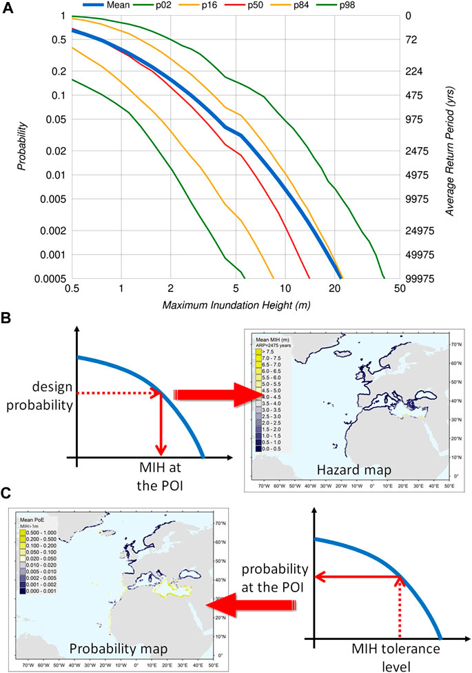
FIGURE 10. (A) Example of an ensemble of hazard curves calculated for a point of interest. Each curve represents a different percentile of all the models spanning the epistemic uncertainty. (B) Hazard map (Figure 11A) produced to show the values of the maximum inundation height (MIH, in meters) at any point of interest (POI), obtained by cutting hazard curves at a given design probability of exceedance in 50 years. (C) Probability map (Figure 11A) produced to show the probability of exceedance in 50 years at any point of interest, obtained by cutting hazard curves at a given tolerance level of the maximum inundation height.

Probability and frequency are linked together so that each PoE value corresponds to an ARP, which is the average time between two consecutive events of the same intensity. The adopted exposure time is 50 years, whereas the adopted hazard intensity measure (or metric) is the tsunami MIH evaluated at a POI, representing the coastal stretch behind the POI itself. A single MIH value at a single POI represents an estimate of the mean value along the coast because the actual MIH values vary laterally along the coast behind the POI. Based on our methodological analysis, local maxima of the actual MIH (and maximum run-up) values along the coast are expected not to exceed three-to-four times the mean MIH estimated at the POI. More details on MIH and its lateral variability can be found in Glimsdal et al. (2019).

Six hazard curves are shown in a single plot to represent the model uncertainty. Each curve corresponds to a different statistics of the model uncertainty represented by the hazard curve distribution (Figure 10A). The hazard curves are reported for the mean, and the 2nd, 16th, 50th, 84th, and 98th percentiles of the model ensemble. PoE can be considered robust in the range 10⁻³–10⁰ (ARP<∼50,000 years). Results for PoE < 5 × 10^–4 (ARP >∼100,000 years) are not considered sufficiently well constrained, for example, due to the period covered by the seismic catalogs. Consequently, they are omitted from the results.

Hazard (intensity) and probability maps are derived from hazard curves in which each POI is assigned a value according to the hazard intensity or PoE, respectively (Figures 10B,C). To make a hazard map, we extract the MIH corresponding to a chosen design PoE, or, equivalently, to a given ARP for each POI. To make a probability map, we extract the PoE in 50 years, corresponding to a chosen MIH value for each POI. In either case, map values are calculated by linear interpolation between the two closest points in the hazard curves. Based on this scheme, we put together a portfolio of probability maps for MIH of 1, 2, 5, 10, and 20 m, and hazard intensity maps for ARP of 500, 1,000, 2,500, 5,000, and 10,000 years, that can be navigated in the NEAMTHM18 web interactive tool (Supplementary Figure S6). Different views can be obtained for each map considering the mean or any of the percentiles of the epistemic uncertainty stored in the hazard curves. Figure 11 shows two examples of such maps.

FIGURE 11

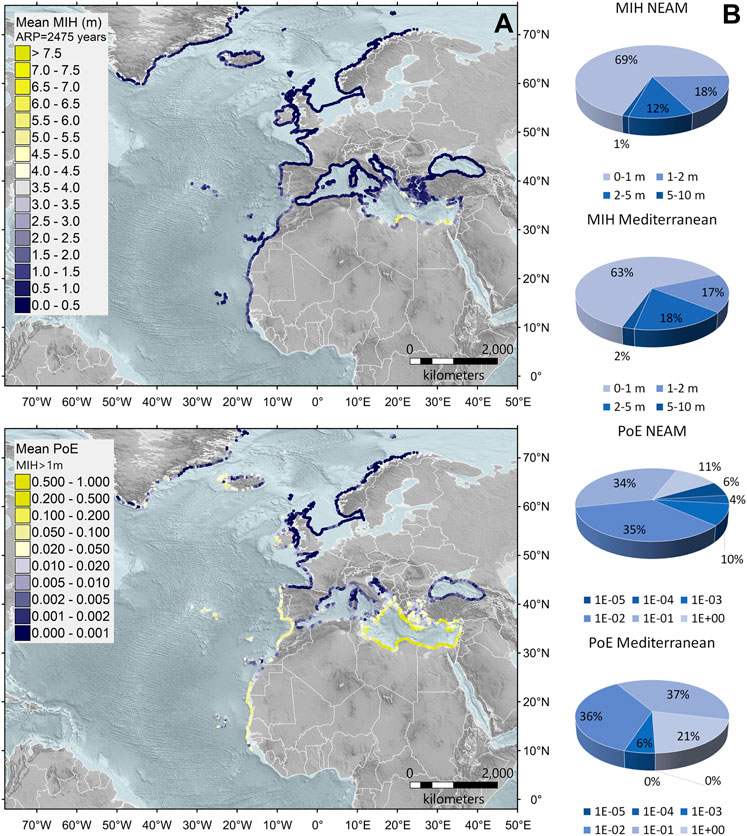
FIGURE 11. (A) NEAMTHM18 hazard map for the probability of exceedance of 2% in 50 years, equivalent to an average return period of 2,475 years (upper) and NEAMTHM18 probability map for maximum inundation height larger than 1 m (lower). Topo-bathymetry is from the ETOPO1 Global Relief Model (NOAA, 2009; Amante and Eakins, 2009). (B) Pie charts showing the percentage of points of interest in the NEAM and Mediterranean coastlines that correspond to different maximum inundation heights for an average return period of 2,475 years (two upper charts) and to different probabilities of exceedance of a maximum inundation height of 1 m (two lower charts). Notice the increasing proportion of points of interest with higher hazard in the Mediterranean region relative to the entire NEAM Region.

Discussion

Tsunami waves can travel long distances without dispersing much energy. Therefore, a relatively high hazard can affect places far from the earthquake source that generated the tsunami. The Caribbean subduction is one of these cases that contributes to the tsunami hazard of European and African coastlines in the Atlantic Ocean. Within the Mediterranean Sea, seismic sources are always much closer to most coastlines than in the Atlantic Ocean. Nonetheless, tsunami hazards can also be high in zones known for not hosting significant seismic sources. For example, although Libya and Egypt do not have hazardous seismic sources, probability maps show that their coastlines are more likely to be affected by significant tsunamis than the coastlines of southern Italy, Greece, Turkey, and Cyprus–all regions located much closer to the subduction zones (Figures 5, 11A). In other words, unlike other types of earthquake-related hazards, both local and distant seismic sources contribute to earthquake-generated tsunami hazards. Although the closeness to seismic sources is undoubtedly a good proxy for a relatively high tsunami hazard, the distance from seismic sources is not necessarily a proxy for a very low tsunami hazard.

An added value of a region-wide hazard computed in a consistent manner is that the hazard of different and very distant places, or even separate basins, can be compared at a glance, without having to worry about how much the hazard depends on the different input datasets or different methods adopted for the calculations. Although regional-scale models cannot replace in-depth analyses at sub-regional (national) and local levels, they can provide a common reference for performing local hazard quantifications focused on different areas (e.g., Bacchi et al., 2020). They also enable using unsupervised filters of seismic sources for more detailed local analyses (Lorito et al., 2015; Volpe et al., 2019) (Supplementary Data Sheet 1.3).

Concerning the mean model for the ARP = 2,475 years, the number of POIs with MIH > 5 m remains within 1% of the entire NEAM Region. Over 30% of the POIs, however, correspond to an MIH > 1 m (Figure 11B), which with local fluctuations may lead to run-ups three times higher (Glimsdal et al., 2019). The NEAM Region is very large and includes coasts facing zones of relatively low seismicity. If we repeat the analysis only for the Mediterranean Sea, we find a larger incidence of potentially destructive events. Similar reasoning can be repeated for the PoE for a given MIH. MIH > 5 m is found only in the Mediterranean Sea. Specifically, in Cyrenaica (Libya), the Nile Delta (Egypt), Cyprus, and the Peloponnese (Greece). In the North-East Atlantic, the highest MIHs are generally lower than those in the Mediterranean Sea. MIH > 3 m is found only in a few locations, such as the Dakhlet Nouadhibou Bay (Mauritania), likely because of the Arguin Spur in the near offshore, and the Gulf of Cadiz (Figure 12).

FIGURE 12

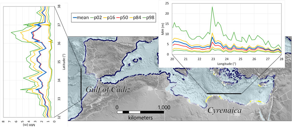
FIGURE 12. Example profiles of the maximum inundation height (MIH; mean and the epistemic uncertainty represented by the 2nd, 16th, 50th, 84th, and 98th percentiles) along coastlines among those with the highest hazard of the NEAM Region. The two profiles span coast of the Gulf of Cadiz (N–S) and the Cyrenaica (E–W). Both profiles are with reference to the hazard model with the 2% probability of exceedance in 50 years (average return period of 2,475 years). The color scale in the map is as in Figure 11. Topo-bathymetry is from the ETOPO1 Global Relief Model (NOAA, 2009; Amante and Eakins, 2009).

When comparing hazard values in different localities, one should always consider uncertainty. Even if two places have the same mean hazard, the actual hazard can differ for different epistemic uncertainty levels. The spreading of the hazard curves at every POI conveys information about the uncertainty that affects these estimates. This fact can be expressed by the relative uncertainty of the MIH or PoE values corresponding to a given percentile around the mean. Figure 13A shows the geographic distributions of an example of the relative uncertainty calculated as the proportion of the 84th percentile with respect to the mean. In other words, this quantifies how much the mean values in the maps of Figure 11A can be overtaken if the 84th percentile of the epistemic uncertainty occurs. Geographically, the impact of the epistemic uncertainty varies significantly. For example, the existing uncertainty on the Gibraltar Arc subduction interface (modeled as SBS type in Step-1) is reflected by significantly distant hazard curves in the Gulf of Cadiz. Figure 13B shows that for most POIs (∼67%), MIH values up to 40% larger than the mean can occur if alternative, though scientifically acceptable, interpretations are considered. The same reasoning applies to the relative uncertainty of the probability associated with specific MIH values.

FIGURE 13

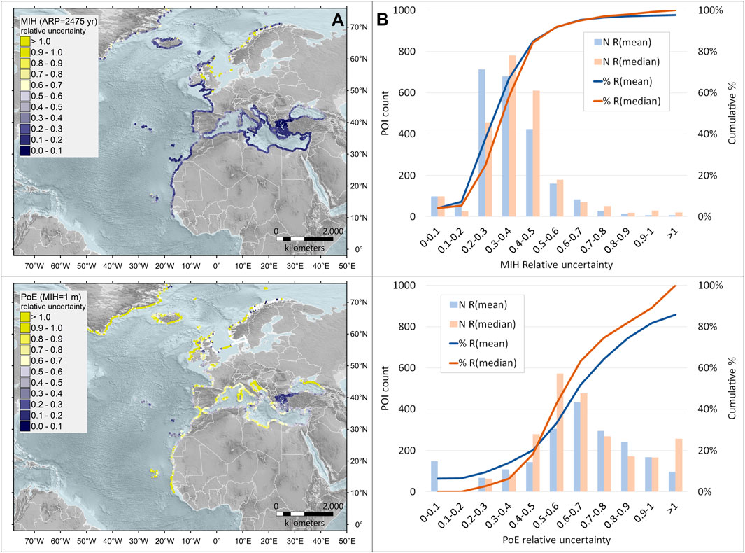
FIGURE 13. (A) Geographic distributions of the maximum inundation height (MIH) relative uncertainty, defined as the ratio R=(MIH_p84-MIH_mean)/MIH_mean, for the 2% probability of exceedance in 50 years, equivalent to an average return period of 2,475 years (upper), and of the probability of exceedance relative uncertainty, defined as the ratio R=(PoE_p84-PoE_mean)/PoE_mean, for the maximum inundation height of 1 m (lower). Topo-bathymetry is from the ETOPO1 Global Relief Model (NOAA, 2009; Amante and Eakins, 2009). (B) Incremental and cumulative distribution of the relative uncertainty as defined in panel (A) for MIH (upper) and PoE (lower). For comparison, both diagrams also show the relative uncertainty with respect to the median.

In the entire NEAM Region, catastrophic events, such as those that can produce MIHs larger than several meters, are rare but not impossible. The highest tsunami hazard of the NEAM Region is found in the central-eastern Mediterranean, where long stretches of the coastline can exceed an MIH of 5 m with significant probability, and with lower probability in the region of the Gulf of Cadiz. In the latter, much of the hazard is likely driven by the Gibraltar Arc subduction interface. As discussed above, the epistemic uncertainty in this region can be reduced by improving the subduction interface characterization.

In NEAMTHM18, the model uncertainties have been addressed together with the PE through two elicitation experiments (Figure 1). The first elicitation experiment was devoted to identifying and prioritizing the possible alternative model implementations at all Steps and Levels (Supplementary Table S1). However, the list of specific aspects of each alternative could even be much longer than reported and possibly include cases of alternatives that became available after the first elicitation experiment but could not be implemented in the timeframe of the project. Some of these alternatives were also specifically suggested by the IR during the review phases (Figure 1), but their implementation was not feasible with the available data and resources.

At Step-1, for example, the SLAB two model (Hayes et al., 2018) represents a possible alternative for the geometry of subduction interfaces (PS type). Likewise, large crustal faults with sufficient information (3D geometry and tectonic rates) could be addressed in the PS type rather than the BS type. Using tectonic rates for the BS type would increase the FMD model alternatives, contributing to better addressing the long recurrence intervals of major crustal earthquakes as done for the PS type. As regards the earthquake ruptures, the modeling could explore the use of recent rupture scaling relations, such as those by Goda et al. (2016), Allen and Hayes (2017), and Thingbaijam et al. (2017), in addition to those used here. The coseismic slip distribution on such ruptures could also better reflect the open discussion on how best to describe the slip spectra (Herrero and Bernard, 1994; Somerville et al., 1999; Mai and Beroza, 2002; Goda et al., 2016). Our choice of a self-similar slip distribution was based on its consistency with the use of a stress drop that does not scale with the seismic moment, a feature that has been observed over a large range of magnitudes (Cocco et al., 2016). It may also be noted that we used heterogeneous slip distributions only for the largest earthquakes on subduction interfaces. Since slip heterogeneity may affect tsunami hazard even at large distances from the fault (e.g., Li et al., 2016), future model updates might consider developing heterogeneous slip distributions not only for large subduction interface earthquakes but also for smaller earthquakes and at least for the largest crustal sources. At Step-2, other possible improvements in modeling different aspects of the seismic sources would improve the tsunamigenic efficiency characterization of each considered earthquake scenario. Examples of such improvements are the description of the Earth’s model in which the source is embedded (Masterlark, 2003; Romano et al., 2015b), the consideration of time-dependent ruptures, and of the mechanism of transmission of the coseismic seafloor displacement to the water column (e.g., Tanioka and Satake, 1996; Nosov and Kolesov, 2011; Polet and Kanamori, 2015; Geist et al., 2019). It is also worth noting that further uncertainties also affect Step-2 and Step-3 due to the limited accuracy of the topo-bathymetric model and the numerical simulations with the Tsunami-HySEA code solving the NLSW equations. These additional uncertainties, and some of the above-mentioned uncertainties on tsunami generation, have been implicitly embedded in the amplification factors. Although rather roughly, they contribute to the log-normal distribution combined to the deterministic output of each single tsunami simulation as described for Step-3 and Step-4, based on the calibration made by Glimsdal et al. (2019) by means of numerical simulations. A similar approach, though based on tsunami observations, was previously adopted by Davies et al. (2018).

A probabilistic hazard model attempts to forecast future hazards at a location, but this prediction will never be an exact representation of the reality or precisely anticipate the occurrence of a specific hazardous event. The inherent uncertainty of such predictions is rooted in the limited understanding of natural phenomena and the lack of data to build models, as recalled above. In general, the longer the ARP, the scarcer the observations for building and testing the model. The large uncertainty of tsunami hazard models is strongly related to the fact that tsunamis are rather low-frequency but potentially high-impact events. Therefore, in comparison with hazard models for more frequent phenomena, tsunami hazard models have typically even scarcer observations that can be used for their calibration, perhaps except for the Pacific Ocean (Geist and Parsons, 2016). Accordingly, and following common practices (Geist and Lynett, 2014; Grezio et al., 2017), the NEAMTHM18 was built by modeling earthquake probability and tsunami generation and impact from these earthquakes, rather than building it directly from available tsunami observations, which is an almost impossible task for tsunamis. NEAMTHM18 also considers potential unknown events whose occurrence cannot be ruled out for the future. Tsunami data, such as long records of a measured run-up at a specific coastal site, are even scarcer in the NEAM Region than in other regions characterized by more frequent (large) earthquakes, as may be the case for Chile. All the circumstances mentioned above suggest caution when using hazard results for practical applications, particularly for long ARPs.

Building on the legacy of recent European research projects dedicated to developing data and methods for tsunami hazard analysis and other hazards, the TSUMAPS-NEAM (2016–2017) project has brought about NEAMTHM18, the first long-term tsunami hazard assessment for the NEAM Region. Scientific and technical advancements are required to perform effective hazard analyses. This work is carried out by specialists of different disciplines and is never finalized. It is instead a never-ending process, as schematically illustrated in Figure 14. One full round of this circle may take several years to be completed. At each new round, hazard maps can be better. NEAMTHM18 represents the body of results in point 3 of Figure 14. The preceding points 1 and 2 (Figure 14) were completed in the framework of the TSUMAPS-NEAM project but started well before in other projects that were not necessarily dedicated to tsunami hazard alone, such as TRANSFER (2006–2009), SHARE (2009–2012), STREST (2013–2016), and ASTARTE (2013–2017) (Table 1), each of which contributed with the preparation of relevant datasets, with the development of methods, and, most importantly, with the building of a large community. Only a few actions are now needed to complete the first round of this circle. Disaggregation and sensitivity analyses have already been performed and are part of the NEAMTHM18 Documentation (Basili et al., 2019). Expanding and exploiting those analyses will eventually lead to a new round of improvements to the tsunami hazard model. Discussions aimed at establishing best practices in this respect are in progress within the GTM scientific network and its related AGITHAR COST Action. Successive hazard projects will use better data and newer methods. They will also exploit technological advancements and innovations, such as the enhanced performances of computer systems that will allow more complex approaches to be explored, like in the ongoing ChEESE project, thereby improving the capability to develop appropriate protection and resilience measures against tsunamis.

FIGURE 14

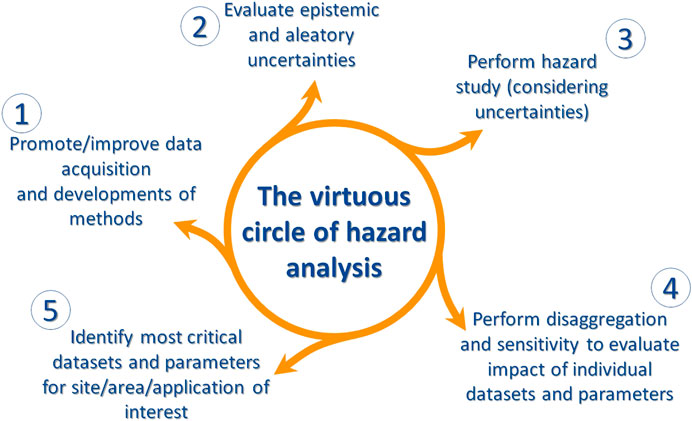
FIGURE 14. The virtuous circle of hazard analysis.

Data Availability Statement

The datasets presented in this study can be found in online repositories. The names of the repository/repositories and accession number(s) can be found below: NEAM Tsunami Hazard Model 2018 (NEAMTHM18): online data of the Probabilistic Tsunami Hazard Model for the NEAM Region from the TSUMAPS-NEAM project, http://doi.org/10.13127/tsunami/neamthm18; NEAMTHM18 Documentation: the making of the TSUMAPS-NEAM Tsunami Hazard Model 2018, http://doi.org/10.5281/zenodo.3406625.

Author Contributions

AAg, ABa, ABo, AHe, AHo, AS, AY, BB, CBH, FC, FEM, FL, FO, FR, GL, GP, HAJ, HH, HKT, IT, JS, LMM, MAB, MC, MGu, MMT, MT, MV, OP, PP, RB, RO, RT, SB, SBA, SG, SI, SL, and SM contributed to developing NEAMTHM18 as members of the Project Development Team. RB coordinated the TSUMAPS-NEAM project. SL led the project management and reporting, assisted by BB. JS and RO led the hazard assessment task. ABa and GP led the review and sanity check task. OP led the dissemination task. OP and MGu developed the interactive hazard curve tool. JMGV and JMS provided support with the use of the Tsunami-HySEA code. FR, RO, FL, ABa, AY, GP, MC, ABo, AAr, MS, COS, GD, WP, JP, and CM were members of the Pool of Experts. JB, DDB, MD, MP, AAm, AZ, MGo, JMGV, EG, JMS, and TP were members of the panel of Internal Reviewers. All authors participated in one or more project meetings, in person or remotely, to contribute to or discuss various aspects of the NEAMTHM18. RB, SL, and JS prepared the first draft of the manuscript. All authors read and variably contributed to revising the manuscript.

Funding

The NEAMTHM18 was prepared in the framework of the European Project TSUMAPS-NEAM (http://www.tsumaps-neam.eu/) funded by the mechanism of the European Civil Protection and Humanitarian Aid Operations with grant no. ECHO/SUB/2015/718568/PREV26 (https://ec.europa.eu/echo/funding-evaluations/financing-civil-protection-europe/selected-projects/probabilistic-tsunami-hazard_en). The work by INGV authors also benefitted from funding by the INGV-DPC Agreement 2012-2021 (Annex B2).

Conflict of Interest

Author HKT is employed by AECOM Technical Services, United States; author AHo is now employed at Gempa GmbH, Potsdam, Germany, but was employed at GFZ German Research Centre for Geosciences, Potsdam, Germany, while working on the project.

The remaining authors declare that the research was conducted in the absence of any commercial or financial relationships that could be construed as a potential conflict of interest.

Acknowledgments

We acknowledge the valuable contributions of all the scientists, end-users, and stakeholders who actively participated in the TSUMAPS-NEAM project meetings. We also acknowledge the constructive comments made by the reviewers, which contributed to significantly improve the quality of the paper. Tsunami modeling was done with the HPC support by EDANYA Group (https://www.uma.es/edanya), Universidad de Málaga, Spain, that made the Tsunami-HySEA code available, and by CINECA Consortium (https://www.cineca.it/en) that provided access to their facilities.

Supplementary Material

The Supplementary Material for this article can be found online at: https://www.frontiersin.org/articles/10.3389/feart.2020.616594/full#supplementary-material.

References

Aki, K., and Richards, P. G. (1980). Quantitative seismology: theory and methods. San Francisco, CA: Freeman.

Allen, T. I., and Hayes, G. P. (2017). Alternative rupture‐scaling relationships for subduction interface and other offshore environments. Bull. Seismol. Soc. Am. 107, 1240–1253. doi:10.1785/0120160255

CrossRef Full Text | Google Scholar

Álvarez-Gómez, J. A., Aniel-Quiroga, ĺ., González, M., and Otero, L. (2011). Tsunami hazard at the Western Mediterranean Spanish coast from seismic sources. Nat. Hazards Earth Syst. Sci. 11, 227–240. doi:10.5194/nhess-11-227-2011

CrossRef Full Text | Google Scholar

Amante, C., and Eakins, B. W. (2009). ETOPO1 1 arc-minute global relief model: procedures, data sources and analysis. NOAA technical memorandum NESDIS NGDC-24. National Geophysical Data Center, NOAA. doi:10.7289/V5C8276M (Accessed December 5, 2020).

Google Scholar

Ambraseys, N. N. (1962). Data for the investigation of the seismic sea-waves in the Eastern Mediterranean. Bull. Seismol. Soc. Am. 52, 895–913.

Google Scholar

American Society of Civil Engineers (2017). Minimum design loads and associated criteria for buildings and other structures. 7th Edn. Reston, VA: American Society of Civil Engineers.

Argyroudis, S. A., Fotopoulou, S., Karafagka, S., Pitilakis, K., Selva, J., Salzano, E., et al. (2020). A risk-based multi-level stress test methodology: application to six critical non-nuclear infrastructures in Europe. Nat. Hazards 100, 595–633. doi:10.1007/s11069-019-03828-5

CrossRef Full Text | Google Scholar

Bacchi, V., Jomard, H., Scotti, O., Antoshchenkova, E., Bardet, L., Duluc, C.-M., et al. (2020). Using meta-models for tsunami hazard analysis: an example of application for the French atlantic coast. Front. Earth Sci. 8, 41. doi:10.3389/feart.2020.00041

CrossRef Full Text | Google Scholar

Bakırcı, T., Yoshizawa, K., and Özer, M. F. (2012). Three-dimensional S-wave structure of the upper mantle beneath Turkey from surface wave tomography: 3-D upper-mantle structure beneath Turkey. Geophys. J. Int. 190, 1058–1076. doi:10.1111/j.1365-246X.2012.05526.x

CrossRef Full Text | Google Scholar

Basili, R., Brizuela, B., Herrero, A., Iqbal, S., Lorito, S., Maesano, F. E., et al. (2018). NEAM tsunami hazard model 2018 (NEAMTHM18): online data of the probabilistic tsunami hazard model for the NEAM region from the TSUMAPS-NEAM project. Roma: Istituto Nazionale di Geofisica e Vulcanologia (INGV). doi:10.13127/tsunami/neamthm18

Basili, R., Brizuela, B., Herrero, A., Iqbal, S., Lorito, S., Maesano, F. E., et al. (2019). NEAMTHM18 documentation: the making of the TSUMAPS-NEAM tsunami hazard model 2018. Roma: Istituto Nazionale di Geofisica e Vulcanologia (INGV), 352. doi:10.5281/Q20zenodo.3406625

CrossRef Full Text | Google Scholar

Basili, R., Kastelic, V., Demircioglu, M. B., Garcia Moreno, D., Nemser, E. S., Petricca, P., et al. (2013a). The European database of seismogenic faults (EDSF) compiled in the framework of the project SHARE. Roma: Istituto nazionale di geofisica e vulcanologia (INGV). doi:10.6092/INGV.IT-SHARE-EDSF Available at: http://diss.rm.ingv.it/share-edsf/ (Accessed July 14, 2020).

Google Scholar

Basili, R., Tiberti, M. M., Kastelic, V., Romano, F., Piatanesi, A., Selva, J., et al. (2013b). Integrating geologic fault data into tsunami hazard studies. Nat. Hazards Earth Syst. Sci. 13, 1025–1050. doi:10.5194/nhess-13-1025-2013

CrossRef Full Text | Google Scholar

Becker, J. J., Sandwell, D. T., Smith, W. H. F., Braud, J., Binder, B., Depner, J., et al. (2009). Global bathymetry and elevation data at 30 arc seconds resolution: SRTM30_PLUS. Mar. Geodes. 32, 355–371. doi:10.1080/01490410903297766

CrossRef Full Text | Google Scholar

Bilek, S. L., and Lay, T. (1999). Rigidity variations with depth along interplate megathrust faults in subduction zones. Nature 400, 443–446. doi:10.1038/22739

CrossRef Full Text | Google Scholar

Bird, P. (2003). An updated digital model of plate boundaries. Geochem. Geophys. Geosyst. 4 (3), 1027. doi:10.1029/2001GC000252

CrossRef Full Text | Google Scholar

Bird, P., and Kagan, Y. Y. (2004). Plate-tectonic analysis of shallow seismicity: apparent boundary width, beta, corner magnitude, coupled lithosphere thickness, and coupling in seven tectonic settings. Bull. Seismol. Soc. Am. 94, 2380–2399. doi:10.1785/0120030107

CrossRef Full Text | Google Scholar

Bommer, J. J. (2012). Challenges of building logic trees for probabilistic seismic hazard analysis. Earthq. Spectra. 28, 1723–1735. doi:10.1193/1.4000079

CrossRef Full Text | Google Scholar

Boyd, O. S. (2012). Including foreshocks and aftershocks in time-independent probabilistic seismic-hazard analyses. Bull. Seismol. Soc. Am. 102, 909–917. doi:10.1785/0120110008

CrossRef Full Text | Google Scholar

Bozzoni, F., Corigliano, M., Lai, C. G., Salazar, W., Scandella, L., Zuccolo, E., et al. (2011). Probabilistic seismic hazard assessment at the eastern caribbean islands. Bull. Seismol. Soc. Am. 101, 2499–2521. doi:10.1785/0120100208

CrossRef Full Text | Google Scholar

Carafa, M. M. C., Kastelic, V., Bird, P., Maesano, F. E., and Valensise, G. (2018). A “geodetic gap” in the Calabrian Arc: evidence for a locked subduction megathrust?. Geophys. Res. Lett. 45, 1794–1804. doi:10.1002/2017gl076554

CrossRef Full Text | Google Scholar

Casarotti, E., Stupazzini, M., Lee, S. J., Komatitsch, D., Piersanti, A., and Tromp, J. (2008). “CUBIT and seismic wave propagation based upon the spectral-element method: an advanced unstructured mesher for complex 3D geological media,” in Proceedings of the 16th international meshing roundtable. Editors M. L. Brewer, and D. Marcum (Berlin, Heidelberg: Springer Berlin Heidelberg), 579–597.

Google Scholar

Cerase, A., Crescimbene, M., La Longa, F., and Amato, A. (2019). Tsunami risk perception in southern Italy: first evidence from a sample survey. Nat. Hazards Earth Syst. Sci. 19, 2887–2904. doi:10.5194/nhess-19-2887-2019

CrossRef Full Text | Google Scholar

Christophersen, A., Berryman, K., and Litchfield, N. (2015). The GEM faulted Earth project, version 1.0, April 2015, GEM faulted Earth project, GEM Foundation, Pavia. doi:10.13117/GEM.GEGD.TR2015.02

Civiero, C., Custódio, S., Duarte, J. C., Mendes, V. B., and Faccenna, C. (2020). Dynamics of the Gibraltar arc system: a complex interaction between plate convergence, slab pull, and mantle flow. J. Geophys. Res. Solid Earth 125, e2019JB018873. doi:10.1029/2019JB018873

CrossRef Full Text | Google Scholar

Cocco, M., Tinti, E., and Cirella, A. (2016). On the scale dependence of earthquake stress drop. J. Seismol. 20, 1151–1170. doi:10.1007/s10950-016-9594-4

CrossRef Full Text | Google Scholar

Cornell, C. A. (1968). Engineering seismic risk analysis. Bull. Seismol. Soc. Am. 58, 1583–1606.

Google Scholar

Davies, G. (2019). Tsunami variability from uncalibrated stochastic earthquake models: tests against deep ocean observations 2006-2016. Geophys. J. Int. 218, 1939–1960. doi:10.1093/gji/ggz260

CrossRef Full Text | Google Scholar

Davies, G., Griffin, J., Løvholt, F., Glimsdal, S., Harbitz, C., Thio, H. K., et al. (2018). A global probabilistic tsunami hazard assessment from earthquake sources. Geological Society, London, Special Publications 456, 219–244. doi:10.1144/sp456.5

CrossRef Full Text | Google Scholar

Davies, G., and Griffin, J. (2020). Sensitivity of probabilistic tsunami hazard assessment to far-field earthquake slip complexity and rigidity depth-dependence: case study of Australia. Pure Appl. Geophys. 177, 1521. doi:10.1007/s00024-019-02299-w

CrossRef Full Text | Google Scholar

DCDPC (2018). Indicazioni alla componenti ed alle strutture operative del Servizio nazionale di protezione civile per l’aggiornamento delle pianificazioni di protezione civile per il rischio maremoto. GU serie generale n.266. del 15–11–2018 (in Italian). Presidenza del consiglio dei ministri—dipartimento della protezione civile. Available at: http://www.protezionecivile.gov.it/amministrazione-trasparente/provvedimenti/dettaglio/-/asset_publisher/default/content/indicazioni-alle-componenti-ed-alle-strutture-operative-del-servizio-nazionale-di-protezione-civile-per-l-aggiornamento-delle-pianificazioni-di-prot-1 (Accessed December 16, 2020).

Google Scholar

de la Asunción, M., Castro, M. J., Fernández-Nieto, E. D., Mantas, J. M., Acosta, S. O., and González-Vida, J. M. (2013). Efficient GPU implementation of a two waves TVD-WAF method for the two-dimensional one layer shallow water system on structured meshes. Comput. Fluids 80, 441–452. doi:10.1016/j.compfluid.2012.01.012

CrossRef Full Text | Google Scholar

Delavaud, E., Cotton, F., Akkar, S., Scherbaum, F., Danciu, L., Beauval, C., et al. (2012). Toward a ground-motion logic tree for probabilistic seismic hazard assessment in Europe. J. Seismol. 16, 451–473. doi:10.1007/s10950-012-9281-z

CrossRef Full Text | Google Scholar

DISS Working Group (2018). Database of individual seismogenic sources (DISS), version 3.2.1. Istituto nazionale di geofisica e vulcanologia (INGV). Available at: http://diss.rm.ingv.it/diss/ (Accessed July 14, 2020). doi:10.6092/INGV.IT-DISS3.2.1

Google Scholar

Duarte, J. C., Rosas, F. M., Terrinha, P., Schellart, W. P., Boutelier, D., Gutscher, M.-A., et al. (2013). Are subduction zones invading the Atlantic? Evidence from the southwest Iberia margin. Geology 41, 839–842. doi:10.1130/G34100.1

CrossRef Full Text | Google Scholar

Dziewonski, A. M., Chou, T.-A., and Woodhouse, J. H. (1981). Determination of earthquake source parameters from waveform data for studies of global and regional seismicity. J. Geophys. Res. 86, 2825–2852. doi:10.1029/JB086iB04p02825

CrossRef Full Text | Google Scholar

Ekström, G., Nettles, M., and Dziewoński, A. M. (2012). The global CMT project 2004-2010: centroid-moment tensors for 13,017 earthquakes. Phys. Earth Planet. In. 200-201, 1–9. doi:10.1016/j.pepi.2012.04.002

CrossRef Full Text | Google Scholar

Esposito, S., Stojadinović, B., Babič, A., Dolšek, M., Iqbal, S., Selva, J., et al. (2020). Risk-based multilevel methodology to stress test critical infrastructure systems. J. Infrastruct. Syst. 26, 04019035. doi:10.1061/(ASCE)IS.1943-555X.0000520

CrossRef Full Text | Google Scholar

Esteva, L. (1967). “Criteria for the construction of spectra for seismic design,” in Third panamerican symposium on structures (Venezuela: Caracas).

Google Scholar

Field, E. H., Arrowsmith, R. J., Biasi, G. P., Bird, P., Dawson, T. E., Felzer, K. R., et al. (2014). Uniform California earthquake rupture forecast, version 3 (UCERF3)--The time-independent model. Bull. Seismol. Soc. Am. 104, 1122–1180. doi:10.1785/0120130164

CrossRef Full Text | Google Scholar

Forman, E., and Peniwati, K. (1998). Aggregating individual judgments and priorities with the analytic hierarchy process. Eur. J. Oper. Res. 108, 165–169. doi:10.1016/S0377-2217(97)00244-0

CrossRef Full Text | Google Scholar

Frankel, A. (1995). Mapping seismic hazard in the central and eastern United States. Seismol Res. Lett. 66, 8–21. doi:10.1785/gssrl.66.4.8

CrossRef Full Text | Google Scholar

Ganas, A., and Parsons, T. (2009). Three-dimensional model of Hellenic Arc deformation and origin of the Cretan uplift. J. Geophys. Res. 114, B06404. doi:10.1029/2008JB005599

CrossRef Full Text | Google Scholar

Gardner, J. K., and Knopoff, L. (1974). Is the sequence of earthquakes in Southern California, with aftershocks removed, Poissonian?. Bull. Seismol. Soc. Am. 64, 1363–1367.

Google Scholar

Geist, E. L. (2012). Phenomenology of tsunamis II. Adv.Geophys. 53, 35–92. doi:10.1016/B978-0-12-380938-4.00002-1

CrossRef Full Text | Google Scholar

Geist, E. L., Oglesby, D. D., and Ryan, K. J. (2019). “Tsunamis: stochastic models of occurrence and generation mechanisms,” in Encyclopedia of complexity and systems science. Editor R. A. Meyers (Berlin, Heidelberg: Springer Berlin Heidelberg), 1–30.

CrossRef Full Text | Google Scholar

Geist, E. L., and Parsons, T. (2006). Probabilistic analysis of tsunami hazards*. Nat. Hazards 37, 277–314. doi:10.1007/s11069-005-4646-z

CrossRef Full Text | Google Scholar

Geist, E. L., and Parsons, T. (2016). Reconstruction of far-field tsunami amplitude distributions from earthquake sources. Pure Appl. Geophys. 173, 3703–3717. doi:10.1007/s00024-016-1288-x

CrossRef Full Text | Google Scholar

Geist, E., and Lynett, P. (2014). Source processes for the probabilistic assessment of tsunami hazards. Oceanog. 27, 86–93. doi:10.5670/oceanog.2014.43

CrossRef Full Text | Google Scholar

Gerstenberger, M. C., Marzocchi, W., Allen, T., Pagani, M., Adams, J., Danciu, L., et al. (2020). Probabilistic seismic hazard analysis at regional and national scales: state of the art and future challenges. Rev. Geophys. 58. doi:10.1029/2019RG000653

CrossRef Full Text | Google Scholar

Gibbons, S. J., Lorito, S., Macías, J., Løvholt, F., Selva, J., Volpe, M., et al. (2020). Probabilistic tsunami hazard analysis: high performance computing for massive scale inundation simulations. Front. Earth Sci. 8, 623. doi:10.3389/feart.2020.591549

CrossRef Full Text | Google Scholar

Glimsdal, S., Løvholt, F., Harbitz, C. B., Romano, F., Lorito, S., Orefice, S., et al. (2019). A new approximate method for quantifying tsunami maximum inundation height probability. Pure Appl. Geophys. 176, 3227–3246. doi:10.1007/s00024-019-02091-w

CrossRef Full Text | Google Scholar

Goda, K., Yasuda, T., Mori, N., and Maruyama, T. (2016). New scaling relationships of earthquake source parameters for stochastic tsunami simulation. Coast Eng. J. 58, 1650010–1650011. doi:10.1142/S0578563416500108

CrossRef Full Text | Google Scholar

González, F. I., Geist, E. L., Jaffe, B., Kânoğlu, U., Mofjeld, H., Synolakis, C. E., et al. (2009). Probabilistic tsunami hazard assessment at Seaside, Oregon, for near- and far-field seismic sources. J. Geophys. Res. 114, C11023. doi:10.1029/2008JC005132

CrossRef Full Text | Google Scholar

Grezio, A., Marzocchi, W., Sandri, L., and Gasparini, P. (2010). A bayesian procedure for probabilistic tsunami hazard assessment. Nat. Hazards 53, 159–174. doi:10.1007/s11069-009-9418-8

CrossRef Full Text | Google Scholar

Grezio, A., Sandri, L., Marzocchi, W., Argnani, A., Gasparini, P., and Selva, J. (2012). Probabilistic tsunami hazard assessment for Messina strait area (sicily, Italy). Nat. Hazards 64, 329–358. doi:10.1007/s11069-012-0246-x

CrossRef Full Text | Google Scholar

Grezio, A., Roberto, T., Sandri, L., Pierdominici, S., and Selva, J. (2015). A methodology for a comprehensive probabilistic tsunami hazard assessment: multiple sources and short-term interactions. J. Mar. Sci. Eng. 3, 23–51. doi:10.3390/jmse3010023

CrossRef Full Text | Google Scholar

Grezio, A., Babeyko, A., Baptista, M. A., Behrens, J., Costa, A., Davies, G., et al. (2017). Probabilistic tsunami hazard analysis: multiple sources and global applications. Rev. Geophys. 55, 1158–1198. doi:10.1002/2017rg000579

CrossRef Full Text | Google Scholar

Grünthal, G., and Wahlström, R. (2012). The European-Mediterranean Earthquake Catalogue (EMEC) for the last millennium. J. Seismol. 16, 535–570. doi:10.1007/s10950-012-9302-y

CrossRef Full Text | Google Scholar

Gutscher, M.-A., Malod, J., Rehault, J.-P., Contrucci, I., Klingelhoefer, F., Mendes-Victor, L., et al. (2002). Evidence for active subduction beneath Gibraltar. Geol. 30, 1071–1074. doi:10.1130/0091-7613(2002)030<1071:EFASBG>2.0.CO;2

CrossRef Full Text | Google Scholar

Hayes, G. P., Moore, G. L., Portner, D. E., Hearne, M., Flamme, H., Furtney, M., et al. (2018). Slab2, a comprehensive subduction zone geometry model. Science 362, 58–61. doi:10.1126/science.aat4723 |

PubMed Abstract | CrossRef Full Text | Google Scholar

Herrero, A., and Bernard, P. (1994). A kinematic self-similar rupture process for earthquakes. Bull. Seismol. Soc. Am. 84, 1216–1228.

Google Scholar

Herrero, A., and Murphy, S. (2018). Self-similar slip distributions on irregular shaped faults. Geophys. J. Int. 213, 2060–2070. doi:10.1093/gji/ggy104

CrossRef Full Text | Google Scholar

Hiemer, S., Woessner, J., Basili, R., Danciu, L., Giardini, D., and Wiemer, S. (2014). A smoothed stochastic earthquake rate model considering seismicity and fault moment release for Europe. Geophys. J. Int. 198, 1159–1172. doi:10.1093/gji/ggu186

CrossRef Full Text | Google Scholar

Howell, A., Jackson, J., Copley, A., McKenzie, D., and Nissen, E. (2017). Subduction and vertical coastal motions in the eastern Mediterranean. Geophys. J. Int. 211, 593–620. doi:10.1093/gji/ggx307

CrossRef Full Text | Google Scholar

Iervolino, I., Giorgio, M., and Polidoro, B. (2012). Paper No. 66. “Probabilistic seismic hazard analysis for seismic sequences,” in VEESD 2013, Vienna congress on recent advances in earthquake engineering and structural dynamics 2013, Vienna, Austria, August 28-30, 2013. Editors C. Adam, R. Heuer, W. Lenhardt, and C. Schranz (Vienna, Austria: OGE Vienna University of Technology). Available at: https://veesd2013.conf.tuwien.ac.at/about.html

Google Scholar

IOC (2015). Working Group on Tsunamis and Other Hazards Related to Sea-Level Warning and Mitigation Systems (TOWS-WG), prepared by the Intergovernmental Oceanographic Commission, Reports of Meetings of Experts and Equivalent Bodies, Eighth Meeting,Morioka, Japan, Morioka, Japan. Available at: https://unesdoc.unesco.org/ark:/48223/pf0000234722?posInSet=1&queryId=N-EXPLORE-2afb4d13-21d9-4c6d-9276-c3de8073f23d (Accessed March 12–13, 2015).

Google Scholar

IOC (2017). Plans and procedures for tsunami warning and emergency management. Paris: Intergovernmental Oceanographic Commission of UNESCO.

ISC (2016). On-line bulletin. International seismological centre. Available at: http://www.isc.ac.uk. (Accessed November 3, 2018).

Google Scholar

Kagan, Y. Y. (2017). Earthquake number forecasts testing. Geophys. J. Int. 211, 335–345. doi:10.1093/gji/ggx300

CrossRef Full Text | Google Scholar

Kagan, Y. Y. (2002a). Seismic moment distribution revisited: I. Statistical results. J. Intell. 148, 520–541. doi:10.1046/j.1365-246x.2002.01594.x

CrossRef Full Text | Google Scholar

Kagan, Y. Y. (2002b). Seismic moment distribution revisited: II. Moment conservation principle. Geophys. J. Int. 149, 731–754. doi:10.1046/j.1365-246X.2002.01671.x

CrossRef Full Text | Google Scholar

Kagan, Y. Y., Bird, P., and Jackson, D. D. (2010). Earthquake patterns in diverse tectonic zones of the globe. Pure Appl. Geophys. 167, 721–741. doi:10.1007/s00024-010-0075-3

CrossRef Full Text | Google Scholar

Kajiura, K. (1963). The leading wave of a tsunami. Bull. Earthq. Res. Inst. Univ. Tokyo 41, 535–571.

Google Scholar

Kamigaichi, O. (2011). “Tsunami forecasting and warning,” in Extreme environmental events. Editor R. A. Meyers (New York, NY: Springer New York), 982–1007.

CrossRef Full Text | Google Scholar

Laigle, M., Sachpazi, M., and Hirn, A. (2004). Variation of seismic coupling with slab detachment and upper plate structure along the western Hellenic subduction zone. Tectonophysics 391, 85–95. doi:10.1016/j.tecto.2004.07.009

CrossRef Full Text | Google Scholar

Laske, G., Masters, G., Ma, Z., and Pasyanos, M. (2013). Update on CRUST1.0—a 1-degree global model of Earth’s crust. Geophys. Res. Abstr. 15, EGU2013–2658.

Google Scholar

Leonard, M. (2014). Self-consistent earthquake fault-scaling relations: update and extension to stable continental strike-slip faults. Bull. Seismol. Soc. Am. 104, 2953–2965. doi:10.1785/0120140087

CrossRef Full Text | Google Scholar

Li, L., Switzer, A. D., Chan, C.-H., Wang, Y., Weiss, R., and Qiu, Q. (2016). How heterogeneous coseismic slip affects regional probabilistic tsunami hazard assessment: a case study in the South China Sea. J. Geophys. Res. Solid Earth 121, 6250–6272. doi:10.1002/2016JB013111

CrossRef Full Text | Google Scholar

Lin, I.-C., and Tung, C. C. (1982). A preliminary investigation of tsunami hazard. Bull. Seismol. Soc. Am. 72, 2323–2337.

Google Scholar

Lorito, S., Selva, J., Basili, R., Romano, F., Tiberti, M. M., and Piatanesi, A. (2015). Probabilistic hazard for seismically induced tsunamis: accuracy and feasibility of inundation maps. Geophys. J. Int. 200, 574–588. doi:10.1093/gji/ggu408

CrossRef Full Text | Google Scholar

Lorito, S., Romano, F., and Lay, T. (2016). “Tsunamigenic major and great earthquakes (2004–2013): source processes inverted from seismic, geodetic, and sea-level data,” in Encyclopedia of complexity and systems science. Editor R. A. Meyers (Berlin, Heidelberg: Springer Berlin Heidelberg), 1–52.

CrossRef Full Text | Google Scholar

Løvholt, F., Glimsdal, S., Harbitz, C. B., Zamora, N., Nadim, F., Peduzzi, P., et al. (2012). Tsunami hazard and exposure on the global scale. Earth Sci. Rev. 110, 58–73. doi:10.1016/j.earscirev.2011.10.002

CrossRef Full Text | Google Scholar

Løvholt, F., Griffin, J., and Salgado-Gálvez, M. A. (2015). “Tsunami hazard and risk assessment on the global scale,” in Encyclopedia of Complexity and systems science. Editor R. A. Meyers (Berlin, Heidelberg: Springer), 1–34.

Google Scholar

Lynett, P. J., Gately, K., Wilson, R., Montoya, L., Arcas, D., Aytore, B., et al. (2017). Inter-model analysis of tsunami-induced coastal currents. Ocean Model. 114, 14–32. doi:10.1016/j.ocemod.2017.04.003

CrossRef Full Text | Google Scholar

Macías, J., Castro, M. J., and Escalante, C. (2020a). Performance assessment of the Tsunami-HySEA model for NTHMP tsunami currents benchmarking. Laboratory data. Coast Eng. 158, 103667. doi:10.1016/j.coastaleng.2020.103667

CrossRef Full Text | Google Scholar

Macías, J., Castro, M. J., Ortega, S., and González-Vida, J. M. (2020b). Performance assessment of Tsunami-HySEA model for NTHMP tsunami currents benchmarking. Field cases. Ocean Model. 152, 101645. doi:10.1016/j.ocemod.2020.101645

CrossRef Full Text | Google Scholar

Macías, J., Castro, M. J., Ortega, S., Escalante, C., and González-Vida, J. M. (2017). Performance benchmarking of tsunami-HySEA model for NTHMP’s inundation mapping activities. Pure Appl. Geophys. 174, 3147–3183. doi:10.1007/s00024-017-1583-1

CrossRef Full Text | Google Scholar

Maesano, F. E., Tiberti, M. M., and Basili, R. (2017). The calabrian arc: three-dimensional modelling of the subduction interface. Sci. Rep. 7, 8887. doi:10.1038/s41598-017-09074-8 |

PubMed Abstract | CrossRef Full Text | Google Scholar

Mai, P. M., and Beroza, G. C. (2002). A spatial random field model to characterize complexity in earthquake slip. J. Geophys. Res. 107 (B11), 10. doi:10.1029/2001JB000588

CrossRef Full Text | Google Scholar

Maramai, A., Brizuela, B., and Graziani, L. (2014). The Euro-Mediterranean Tsunami catalogue. Ann. Geophys. 57(4), S0435. doi:10.4401/ag-6437

Google Scholar

Marzocchi, W., Taroni, M., and Selva, J. (2015). Accounting for epistemic uncertainty in PSHA: logic tree and ensemble modeling. Bull. Seismol. Soc. Am. 105, 2151–2159. doi:10.1785/0120140131

CrossRef Full Text | Google Scholar

Marzocchi, W., and Taroni, M. (2014). Some thoughts on declustering in probabilistic seismic-hazard analysis. Bull. Seismol. Soc. Am. 104, 1838–1845. doi:10.1785/0120130300

CrossRef Full Text | Google Scholar

Masterlark, T. (2003). Finite element model predictions of static deformation from dislocation sources in a subduction zone: sensitivities to homogeneous, isotropic, Poisson-solid, and half-space assumptions. J. Geophys. Res. 108, 2540. doi:10.1029/2002JB002296

CrossRef Full Text | Google Scholar

MCDEM (2016). Tsunami evacuation zones—director’s guideline for civil defence emergency management groups. New Zealand: Ministry of Civil Defence and Emergency Management.

McGuire, R. K. (2008). Probabilistic seismic hazard analysis: early history. Earthq. Eng. Struct. Dynam. 37, 329–338. doi:10.1002/eqe.765

CrossRef Full Text | Google Scholar

Meade, B. J. (2007). Algorithms for the calculation of exact displacements, strains, and stresses for triangular dislocation elements in a uniform elastic half space. Comput. Geosci. 33, 1064–1075. doi:10.1016/j.cageo.2006.12.003

CrossRef Full Text | Google Scholar

Molinari, I., Tonini, R., Lorito, S., Piatanesi, A., Romano, F., Melini, D., et al. (2016). Fast evaluation of tsunami scenarios: uncertainty assessment for a Mediterranean Sea database. Nat. Hazards Earth Syst. Sci. 16, 2593–2602. doi:10.5194/nhess-16-2593-2016

CrossRef Full Text | Google Scholar

Mori, N., Goda, K., and Cox, D. (2018). “Recent process in probabilistic tsunami hazard analysis (PTHA) for mega thrust subduction earthquakes,” in The 2011 Japan Earthquake and tsunami: Reconstruction and restoration advances in natural and technological hazards research. Editors V. Santiago-Fandiño, S. Sato, N. Maki, and K. Iuchi (Cham: Springer International Publishing), 469–485.

CrossRef Full Text | Google Scholar

Munson, C., Stamatakos, J., Juckett, M., Coppersmith, K., and Bommer, J.USNRC (2018). Updated implementation guidelines for SSHAC hazard studies, prepared by JP ake NUREG-2213. Available at: https://www.nrc.gov/reading-rm/doc-collections/nuregs/staff/sr2213/.

Google Scholar

Murotani, S., Satake, K., and Fujii, Y. (2013). Scaling relations of seismic moment, rupture area, average slip, and asperity size for M ∼9 subduction‐zone earthquakes. Geophys. Res. Lett. 40, 5070–5074. doi:10.1002/grl.50976

CrossRef Full Text | Google Scholar

Murphy, S., Di Toro, G., Romano, F., Scala, A., Lorito, S., Spagnuolo, E., et al. (2018). Tsunamigenic earthquake simulations using experimentally derived friction laws. Earth Planet Sci. Lett. 486, 155–165. doi:10.1016/j.epsl.2018.01.011

CrossRef Full Text | Google Scholar

Murphy, S., and Herrero, A. (2020). Surface rupture in stochastic slip models. Geophys. J. Int. 221, 1081–1089. doi:10.1093/gji/ggaa055

CrossRef Full Text | Google Scholar

Murphy, S., Scala, A., Herrero, A., Lorito, S., Festa, G., Trasatti, E., et al. (2016). Shallow slip amplification and enhanced tsunami hazard unravelled by dynamic simulations of mega-thrust earthquakes. Sci. Rep. 6, 35007. doi:10.1038/srep35007 |

PubMed Abstract | CrossRef Full Text | Google Scholar

Nijholt, N., Govers, R., and Wortel, R. (2018). On the forces that drive and resist deformation of the south-central Mediterranean: a mechanical model study. Geophys. J. Int. 214, 876–894. doi:10.1093/gji/ggy144

CrossRef Full Text | Google Scholar

NOAA National Geophysical Data Center (2009). ETOPO1 1 arc-minute global relief model. NOAA National Centers for Environmental Information. Available at: https://www.ngdc.noaa.gov/mgg/global/. (Accessed December 5, 2020).

CrossRef Full Text | Google Scholar

Nosov, M. A., and Kolesov, S. V. (2011). Optimal initial conditions for simulation of seismotectonic tsunamis. Pure Appl. Geophys. 168, 1223–1237. doi:10.1007/s00024-010-0226-6

CrossRef Full Text | Google Scholar

NTC (2018). Norme Tecniche per le Costruzioni 2018. Aggiornamento delle “Norme tecniche per le costruzioni”. Gazzetta Ufficiale Serie Generale n.42 del 2002-2018–suppl. Ordinario n. 8. Italian Building Code (in Italian). Available at: https://www.gazzettaufficiale.it/eli/id/2018/02/20/18A00716/sg (Accessed December 16, 2020).

Google Scholar

Okada, Y. (1992). Internal deformation due to shear and tensile faults in a half-space. Bull. Seismol. Soc. Am. 82, 1018–1040.

Google Scholar

Omira, R., Baptista, M. A., and Matias, L. (2015). Probabilistic tsunami hazard in the northeast atlantic from near- and far-field tectonic sources. Pure Appl. Geophys. 172, 901–920. doi:10.1007/s00024-014-0949-x

CrossRef Full Text | Google Scholar

Papadopoulos, G. A., Daskalaki, E., Fokaefs, A., and Giraleas, N. (2010). Tsunami hazard in the eastern Mediterranean Sea: strong earthquakes and tsunamis in the west Hellenic Arc and trench system. J. Earthquake Tsunami 4, 145–179. doi:10.1142/S1793431110000856

CrossRef Full Text | Google Scholar

Papadopoulos, G. A., Gràcia, E., Urgeles, R., Sallares, V., De Martini, P. M., Pantosti, D., et al. (2014). Historical and pre-historical tsunamis in the Mediterranean and its connected seas: geological signatures, generation mechanisms and coastal impacts. Mar. Geol. 354, 81–109. doi:10.1016/j.margeo.2014.04.014

CrossRef Full Text | Google Scholar

Polet, J., and Kanamori, H. (2015). “Tsunami earthquakes,” in Encyclopedia of complexity and systems science. Editor R. A. Meyers (Berlin, Heidelberg: Springer Berlin Heidelberg), 1–22.

CrossRef Full Text | Google Scholar

Pondrelli, S., and Salimbeni, S. (2015). “Regional moment tensor review: An example from the european–mediterranean region,” in Encyclopedia of Earthquake Engineering. Editors M. Beer, I. A. Kougioumtzoglou, E. Patelli, and I. S.-K. Au (Berlin, Heidelberg: Springer Berlin Heidelberg), 1–15.

CrossRef Full Text | Google Scholar

Power, W., Wang, X., Lane, E., and Gillibrand, P. (2013). A probabilistic tsunami hazard study of the auckland region, Part I: propagation modelling and tsunami hazard assessment at the shoreline. Pure Appl. Geophys. 170, 1621–1634. doi:10.1007/s00024-012-0543-z

CrossRef Full Text | Google Scholar

Reilinger, R., McClusky, S., Vernant, P., Lawrence, S., Ergintav, S., Cakmak, R., et al. (2006). GPS constraints on continental deformation in the Africa-Arabia-Eurasia continental collision zone and implications for the dynamics of plate interactions. J. Geophys. Res. Solid Earth 111, B01405. doi:10.1029/2005JB004051

CrossRef Full Text | Google Scholar

Rikitake, T., and Aida, I. (1988). Tsunami hazard probability in Japan. Bull. Seismol. Soc. Am. 78, 1268–1278.

Google Scholar

Romano, F., Lorito, S., Piatanesi, A., and Lay, T. (2020). Fifteen years of (major to great) tsunamigenic earthquakes. Ref. Module Earth Syst. Environ. Sci. 13. doi:10.1016/B978-0-12-409548-9.11767-1

CrossRef Full Text | Google Scholar

Romano, F., Molinari, I., Lorito, S., and Piatanesi, A. (2015a). Source of the 6 february 2013 Mw = 8.0 santa cruz islands tsunami. Nat. Hazards Earth Syst. Sci. 15, 1371–1379. doi:10.5194/nhess-15-1371-2015

CrossRef Full Text | Google Scholar

Romano, F., Trasatti, E., Lorito, S., Piromallo, C., Piatanesi, A., Ito, Y., et al. (2015b). Structural control on the Tohoku earthquake rupture process investigated by 3D FEM, tsunami and geodetic data. Sci. Rep. 4, 5631. doi:10.1038/srep05631

CrossRef Full Text | Google Scholar

Sørensen, M. B., Spada, M., Babeyko, A., Wiemer, S., and Grünthal, G. (2012). Probabilistic tsunami hazard in the Mediterranean Sea. J. Geophys. Res. Solid Earth 117, B01305. doi:10.1029/2010JB008169

CrossRef Full Text | Google Scholar

Saaty, T. L. (1980). The analytic hierarchy process: planning, priority setting, resource allocation. New York; London: McGraw-Hill International Book Co.

Sachpazi, M., Laigle, M., Charalampakis, M., Diaz, J., Kissling, E., Gesret, A., et al. (2016). Segmented Hellenic slab rollback driving Aegean deformation and seismicity. Geophys. Res. Lett. 43, 651–658. doi:10.1002/2015GL066818

CrossRef Full Text | Google Scholar

Salaün, G., Pedersen, H. A., Paul, A., Farra, V., Karabulut, H., Hatzfeld, D., et al. (2012). High-resolution surface wave tomography beneath the Aegean-Anatolia region: constraints on upper-mantle structure: tomography of Aegea-Anatolia upper mantle. Geophys. J. Int. 190, 406–420. doi:10.1111/j.1365-246X.2012.05483.x

CrossRef Full Text | Google Scholar

Scala, A., Festa, G., Vilotte, J.-P., Lorito, S., and Romano, F. (2019). Wave interaction of reverse‐fault rupture with free surface: numerical analysis of the dynamic effects and fault opening induced by symmetry breaking. J. Geophys. Res. Solid Earth 124, 1743–1758. doi:10.1029/2018jb016512

CrossRef Full Text | Google Scholar

Scala, A., Lorito, S., Romano, F., Murphy, S., Selva, J., Basili, R., et al. (2020). Effect of shallow slip amplification uncertainty on probabilistic tsunami hazard analysis in subduction zones: use of long-term balanced stochastic slip models. Pure Appl. Geophys. 177, 1497–1520. doi:10.1007/s00024-019-02260-x

CrossRef Full Text | Google Scholar

Sellier, N. C., Loncke, L., Vendeville, B. C., Mascle, J., Zitter, T., Woodside, J., et al. (2013a). Post-messinian evolution of the florence ridge area (western Cyprus arc), Part I: morphostructural analysis. Tectonophysics 591, 131–142. doi:10.1016/j.tecto.2012.04.001

CrossRef Full Text | Google Scholar

Sellier, N. C., Vendeville, B. C., and Loncke, L. (2013b). Post-messinian evolution of the florence rise area (western Cyprus arc) Part II: experimental modeling. Tectonophysics 591, 143–151. doi:10.1016/j.tecto.2011.07.003

CrossRef Full Text | Google Scholar

Selva, J., Iqbal, S., Taroni, M., Marzocchi, W., Cotton, F., Courage, W., et al. (2015). Deliverable D3.1: Report on the effects of epistemic uncertainties on the definition of LP-HC events. INGV. Available at: http://strest.ethz.ch/opencms/export/sites/default/.content/STREST_public/STREST_D3.1_updated_151001.pdf (Accessed September 26, 2020).

Google Scholar

Selva, J., and Marzocchi, W. (2004). Focal parameters, depth estimation, and plane selection of the worldwide shallow seismicity with Ms ≥ 7.0 for the period 1900-1976. Geochem. Geophys. Geosystems 5, Q05005. doi:10.1029/2003GC000669

CrossRef Full Text | Google Scholar

Selva, J., and Sandri, L. (2013). Probabilistic seismic hazard assessment: combining cornell-like approaches and data at sites through bayesian inference. Bull. Seismol. Soc. Am. 103, 1709–1722. doi:10.1785/0120120091

CrossRef Full Text | Google Scholar

Selva, J., Tonini, R., Molinari, I., Tiberti, M. M., Romano, F., Grezio, A., et al. (2016). Quantification of source uncertainties in seismic probabilistic tsunami hazard analysis (SPTHA). Geophys. J. Int. 205, 1780–1803. doi:10.1093/gji/ggw107

CrossRef Full Text | Google Scholar

Sodoudi, F., Brüstle, A., Meier, T., Kind, R., Friederich, W., and EGELADOS working group, (2015). Receiver function images of the Hellenic subduction zone and comparison to microseismicity. Solid Earth 6, 135–151. doi:10.5194/se-6-135-2015

CrossRef Full Text | Google Scholar

Somerville, P., Irikura, K., Graves, R., Sawada, S., Wald, D., Abrahamson, N., et al. (1999). Characterizing crustal earthquake slip models for the prediction of strong ground motion. Seismol Res. Lett. 70, 59–80. doi:10.1785/gssrl.70.1.59

CrossRef Full Text | Google Scholar

Strasser, F. O., Arango, M. C., and Bommer, J. J. (2010). Scaling of the source dimensions of interface and intraslab subduction-zone earthquakes with moment magnitude. Seismol Res. Lett. 81, 941–950. doi:10.1785/gssrl.81.6.941

CrossRef Full Text | Google Scholar

Stucchi, M., Rovida, A., Gomez Capera, A. A., Alexandre, P., Camelbeeck, T., Demircioglu, M. B., et al. (2013). The SHARE European earthquake Catalogue (SHEEC) 1000–1899. J. Seismol. 17, 523–544. doi:10.1007/s10950-012-9335-2

CrossRef Full Text | Google Scholar

Tanioka, Y., and Satake, K. (1996). Tsunami generation by horizontal displacement of ocean bottom. Geophys. Res. Lett. 23, 861–864. doi:10.1029/96GL00736

CrossRef Full Text | Google Scholar

Taroni, M., and Selva, J. (in press 2020). GR_EST: an OCTAVE/MATLAB toolbox to estimate Gutenberg-Richter law parameters and their uncertainties. Seismol Res. Lett.

Google Scholar

Thingbaijam, K. K. S., Martin Mai, P., and Goda, K. (2017). New empirical earthquake source‐scaling laws. Bull. Seismol. Soc. Am. 107, 2225–2246. doi:10.1785/0120170017

CrossRef Full Text | Google Scholar

Tiberti, M. M., Basili, R., and Vannoli, P. (2014). Ups and downs in western Crete (Hellenic subduction zone). Sci. Rep. 4, 5677. doi:10.1038/srep05677 |

PubMed Abstract | CrossRef Full Text | Google Scholar

Tinti, S., Armigliato, A., Tonini, R., Maramai, A., and Graziani, L. (2005). Assessing the hazard related to tsunamis of tectonic origin: a hybrid statistical-deterministic method applied to southern Italy coasts. ISET J. Earthq. Technol. 42, 189–201.

Google Scholar

Tonini, R., Basili, R., Maesano, F. E., Tiberti, M. M., Lorito, S., Romano, F., et al. (2020). Importance of earthquake rupture geometry on tsunami modelling: the Calabrian Arc subduction interface (Italy) case study. Geophys. J. Int. 223, 1805–1819. doi:10.1093/gji/ggaa409

CrossRef Full Text | Google Scholar

Tonini, R., Armigliato, A., Pagnoni, G., Zaniboni, F., and Tinti, S. (2011). Tsunami hazard for the city of Catania, eastern sicily, Italy, assessed by means of worst-case credible tsunami scenario analysis (WCTSA). Nat. Hazards Earth Syst. Sci. 11, 1217–1232. doi:10.5194/nhess-11-1217-2011

CrossRef Full Text | Google Scholar

Tozer, B., Sandwell, D. T., Smith, W. H. F., Olson, C., Beale, J. R., and Wessel, P. (2019). Global bathymetry and topography at 15 arc sec: SRTM15+. Earth Space Sci. 6, 1847–1864. doi:10.1029/2019EA000658

CrossRef Full Text | Google Scholar

USNRC (1997). Recommendations for probabilistic seismic hazard analysis: guidance on uncertainty and use of experts, prepared by the SSHAC (senior seismic hazard analysis committee - R.J. Budnitz (chairman), G. Apostolakis, D.M. Boore, L.S. Cluff, K.J. Coppersmith, C.A. Cornell, PA. Morris) NUREG/CR-6372. Available at: https://www.nrc.gov/reading-rm/doc-collections/nuregs/contract/cr6372/vol1/index.html (Accessed September 30, 2020).

Google Scholar

USNRC (2012). Practical implementation guidelines for SSHAC level 3 and 4 hazard studies, prepared by A.M. Kammerer and J.P. Ake, NRC project manager: R. Rivera-Lugo NUREG-2117. Available at: https://www.nrc.gov/reading-rm/doccollections/nuregs/staff/sr2117/ (Accessed September 30, 2020).

Google Scholar

USRNC (2018). Updated implementation guidelines for SSHAC hazard studies, prepared by J. Ake, C. Munson, J. Stamatakos, M. Juckett, K. Coppersmith, and J. Bommer NUREG-2213. Available at: https://www.nrc.gov/reading-rm/doc-collections/nuregs/staff/sr2213/ (Accessed September 30, 2020).

Google Scholar

Vernant, P., Reilinger, R., and McClusky, S. (2014). Geodetic evidence for low coupling on the Hellenic subduction plate interface. Earth Planet Sci. Lett. 385, 122–129. doi:10.1016/j.epsl.2013.10.018

CrossRef Full Text | Google Scholar

Volpe, M., Lorito, S., Selva, J., Tonini, R., Romano, F., and Brizuela, B. (2019). From regional to local SPTHA: efficient computation of probabilistic tsunami inundation maps addressing near-field sources. Nat. Hazards Earth Syst. Sci. 19, 455–469. doi:10.5194/nhess-19-455-2019

CrossRef Full Text | Google Scholar

Wdowinski, S., Ben-Avraham, Z., Arvidsson, R., and Ekström, G. (2006). Seismotectonics of the cyprian arc. Geophys. J. Int. 164, 176–181. doi:10.1111/j.1365-246X.2005.02737.x

CrossRef Full Text | Google Scholar

Wessel, P., Smith, W. H. F., Scharroo, R., Luis, J., and Wobbe, F. (2013). Generic mapping tools: improved version released. Eos Trans. Am. Geophys. Union 94, 409–410. doi:10.1002/2013EO450001

CrossRef Full Text | Google Scholar

Wiemer, S. (2001). A software package to analyze seismicity: ZMAP. Seismol Res. Lett. 72, 373–382. doi:10.1785/gssrl.72.3.373

CrossRef Full Text | Google Scholar

Woessner, J., Laurentiu, D., Giardini, D., Crowley, H., Cotton, F., Grünthal, G., et al. (2015). The 2013 European Seismic Hazard Model: key components and results. Bull. Earthq. Eng. 13, 3553–3596. doi:10.1007/s10518-015-9795-1

CrossRef Full Text | Google Scholar

Woessner, J., and Wiemer, S. (2005). Assessing the quality of earthquake catalogues: estimating the magnitude of completeness and its uncertainty. Bull. Seismol. Soc. Am. 95, 684–698. doi:10.1785/0120040007

CrossRef Full Text | Google Scholar

Zitellini, N., Gràcia, E., Matias, L., Terrinha, P., Abreu, M. A., DeAlteriis, G., et al. (2009). The quest for the Africa–Eurasia plate boundary west of the Strait of Gibraltar. Earth Planet Sci. Lett. 280, 13–50. doi:10.1016/j.epsl.2008.12.005

CrossRef Full Text | Google Scholar