Ionosphere Sounding for Pre-seismic Anomalies Identification (INSPIRE): Results of the Project and Perspectives for the Short-Term Earthquake Forecast

Introduction

The end of the first decade of the third millennium passed under impression from the French satellite DEMETER results. DEMETER was dedicated to the monitoring of ionospheric anomalies appearing around the time of strong earthquakes, in the ionosphere over the areas where earthquake happened (Li and Parrot, 2013; Parrot and Li, 2018). Majority of signals have been registered by satellite several days before the seismic shock, what delivers enough evidence for the existence of the ionospheric precursors of earthquakes. Because of high altitude of DEMETER satellite orbit (in comparison with the altitude of the peak height of the ionosphere), the ionospheric precursor’s proofs were obtained mainly statistically while the GNSS TEC technology, with higher spatial and temporal resolution, provided more and more solid results demonstrating that ionospheric precursors have real practical merit for resolving the problem of the short-term earthquake forecast (Liu et al., 2009; Pulinets et al., 2010; Pulinets et al., 2015; Liu et al., 2018).

Year 2004, when DEMETER satellite was launched, has been marked by one more event–the publication of the monograph where for the first time general problems of ionospheric precursor’s generation mechanism, morphology of this phenomena and technology of their monitoring were thoroughly considered (Pulinets and Boyarchuk, 2004). It was demonstrated in monograph that anomalous variations registered in the ionosphere before earthquakes were reported as early as in 1960s after the Alaska “Good Friday” earthquake (Davies and Baker, 1965). The purposeful studies of ionospheric precursors with the use of ground-based ionosondes started in 1970s (Datchenko et al., 1972) and most convincing results using the satellite technology were obtained using the topside sounding technique (Pulinets, 1998; Pulinets and Legen’ka, 2003). Together with rapidly developing GNSS TEC technology, it is used for the earthquake precursors detection (Liu et al., 2004; Krankowski et al., 2006). Just then word “detection” became the key concept in scientific discussions on how to identify the ionospheric precursors of earthquakes (Dautermann et al., 2007; Thomas et al., 2012).

From the very beginning, the publications on seismo-ionospheric anomalies split into two directions. The first one used the simplest approach associating the observed anomalies with the epicenter position and time of earthquakes (Liu et al., 2004; Kon et al., 2011; Li and Parrot, 2013). However, nobody can guarantee that coincidence with place and time of earthquake confirms that this means the cause-effect relationship. The second approach uses the uniqueness of the physical mechanism generating the seismo-ionospheric anomalies. This uniqueness is a reliable marker for the observed anomaly as related to the earthquake preparation (Pulinets et al., 2003; 2004a; 2007a; Pulinets and Davidenko, 2014; Pulinets and Davidenko, 2018; Davidenko and Pulinets, 2019).

The growing snowball of the publications devoted to the seismo-ionospheric effects initiated the series of international projects aimed to the effect validation. Among them, the European projects should be mentioned. Two simultaneously ongoing FP7 projects: PRE-EARTHQUAKES (Processing Russian and European Earth observations for earthquakes precursors Studies) [http://www.pre-earthquakes.org] and SEMEP (Search for Electro-Magnetic Earthquake Precursors combining satellite and ground-based facilities) with duration through 2013–2015 (http://www.ssg.group.shef.ac.uk/semep/). More representative international project including, except European, the scientists from United States, Japan, Taiwan were organized by the International Space Science Institute (ISSI) in Bern. The project “Multi-instrument Space-Borne Observations and Validation of the Physical Model of the Lithosphere-Atmosphere-Ionosphere-Magnetosphere Coupling” (https://www.issibern.ch/teams/spaceborneobserve/) lasted in 2013–2015 confirmed the validity of the Lithosphere-Atmosphere-Ionosphere Coupling model based on the expertize of the leading scientists working in the area of space physics. As a result of this project the extended AGU Monograph 234 from the Geophysical Monograph Series was published (Ouzounov et al., 2018), including, among others (Pulinets et al., 2018).

Taking into account the success of the DEMETER mission and solid scientific basis of the physical substantiation of the seismo-ionospheric effects, the European Space Agency in 2013 opened the call ESA ITT AO/1–7,548/13/NL/MV for ionospheric sounding for pre-seismic activity identification. One can see that here we encounter the word “identification” what means the main intention of the project to use its results for practical application. This competition was won by the Consortium created by three European institutions: University of Warmia and Mazury in Olsztyn (UWM) as a Prime Contractor, Space Research Center of the Polish Academy of Sciences, and Polytechnic University of Catalonia (UPC), Spain. This project was called INSPIRE (ionosphere Sounding for Pre-seismic anomalies Identification REsearch) and the present paper will be devoted the description of the project results.

Materials and Methods

The effectiveness of the technologies of ionosphere monitoring in ionospheric precursors detection was demonstrated in many researches worldwide. Among them we should mention the vertical ionospheric sounding by ground-based ionosondes (Pulinets et al., 2004b; Liu et al., 2006), by vertical topside sounding from satellites (Pulinets and Legen’ka, 2003), by GNSS TEC monitoring (Liu et al., 2004; 2018), by applying GNSS GIM technique (Liu et al., 2009; Pulinets et al., 2010), by in-situ satellite measurements of the local ionospheric plasma parameters (Parrot and Li, 2018), by low orbit ionospheric tomography (Pulinets et al., 2009; Hirooka et al., 2011), by GNSS occultation technique (Chang et al., 2015), subionospheric VLF waves propagation anomalies (Rozhnoi et al., 2009), oblique ground-based ionospheric sounding (Blaunstein and Hayakawa, 2009), and probably some exotic techniques more. The problem of this diversity is in fact that majority of scientists are working in their own domain and do not imply other techniques. Therefore, the main purpose of the project was the integration of this diversity having in mind searching the most optimal algorithms for the ionospheric precursor’s identification. This means to find the advantages and disadvantages of every technique mentioned above, and to find the most optimal combinations of their application. The second purpose is to demonstrate their common Physical Mechanism, to use the monitoring data not blindly calculating their amplitude outliers and interpreting them as precursor anomalies but finding variations corresponding the dynamical development of the physical processes affecting the ionosphere before earthquakes. And finally, provide recommendations for creating the complex system for Application in the short-term earthquake forecast activity. We consider that the present state of our knowledge and technology is sufficiently advanced for creating of such a system and becomes the matter of political and administrative decisions.

According to the main tasks within the project framework, we provided the analysis of different techniques of the ionosphere monitoring to reveal the limitations of different diagnostic techniques with the purpose of their integration using their advantages. As a test for the physical mechanism validation, we selected the case of L’Aquila M6.3 earthquake on April 6, 2009 in Italy where the extended collected database made it possible to combine different techniques to develop the optimal configuration of the monitoring system. The last part of the project was devoted to the road map definition to create the complex system of the ionosphere monitoring for the task of the short-term earthquake forecast.

One of the crucial points for building the coherent services is validation and unification of different databases in order to mitigate the bias and measurement techniques errors. The currently existing space- and ground-based diagnostics still have a number of gaps in time and space domains. Unfortunately, very often we have to incorporate different type of interpolation and extrapolation methods, which in consequence distort or loose part of the relevant information.

Limitations

Ground based ionosonde stations are distributed essentially sparsely on the globe (in comparison with permanent GNSS stations–few hundreds up to few thousands in each regional network). Absence of the ionosonde stations in the essential seismoactive regions can dramatically limit the proper forecast and we can only study time series of data to reveal anomalous changes in diurnal variability. Sensitivity of the ionosonde to the earthquake precursors is limited by the size of earthquake preparation zone determined by the expression R (km) = 10^0.43 M where M–is the earthquake magnitude (Dobrovolsky et al., 1979). Therefore, it does not allow to study the spatial features and sizes of the anomalies. Due to these reasons, not for all the earthquakes cases the ionosonde data are available.

The range of the oblique sounding ionosondes is essentially larger than vertical ones, but the number of such instruments is even less than the vertical ones. In additions, the functioning of the oblique sounding ionosondes depends on the availability of transmitters providing the proper signal passes over the seismically active regions.

It could sound strange but similar limitation is also characteristic to the network of stationary GNSS receivers for GNSS TEC measurements due to the lack of receivers in ocean regions where many earthquakes take place and in several countries with limited number of receivers. In addition, GNSS TEC data do no permit to observe variations of vertical profiles of electron concentration shape which is an important characteristic of the precursory ionospheric variations.

Topside sounding limitation is common for all techniques of low orbiting satellite monitoring: very limiting time over the monitored regions, and (in case of solar synchronized orbit) inability to monitor precursor’s dynamics in local time.

The in-situ space plasma diagnostics located on board of low orbiting satellite are affected by the same limitations as for the topside sounding satellites. In addition, it is impossible to get the satellite orbit altitude close to the main maximum of the ionosphere (250–350 km). Usually, the satellite orbit is near 600 km and higher (DEMETER satellite), and it is able to observe very tiny variations which could be properly estimated mainly statistically.

For the LEO satellites, using the radio occultation method, the problem is the limitation of observations over a specific region. In general, single satellite passes over specific regions happen only two times per day, with exception of FORMOSAT-3/COSMIC constellation mission providing about 1500 RO daily soundings.

Regardless of the large number of IGS receivers providing GNSS TEC data for GIM technology we still have areas both on the land (for example, Russia, African regions) and over the ocean where we do not have enough receivers to produce accurate maps of electron content. In these regions the real data are either replaced by models or interpolated and we should have some reservation using the GNSS TEC data for ionospheric precursor’s analysis by GIM technology, with a limited space and time resolution.

The VLF subionospheric propagation anomaly diagnostics of signals associated with earthquakes have the same problems as oblique ionospheric sounding and depends on the proper transmitters availability. It could be used only as a proxy detecting the preparation of the earthquake without the determination of the epicenter position.

Low orbiting tomography needs the proper networks of receiving stations whose number is very limited (Romanov et al., 2013), so this technique is still could be regarded as perspective for future years. The tomography based on neural network analysis (Hirooka et al., 2011) needs the dense network of GPS receivers and can be applied only in a limited number of developed countries.

Also incorporation of newly available real-time and near-real time GNSS receivers is sometimes difficult, due to its dependence on many different organizations and infrastructure maintenance cost.

Advantages

Regardless the abovementioned limitations, the vertical sounding probably is the most informative technique of the ionospheric precursors monitoring. The ground-based sounding permits to provide the round the clock state of the ionosphere including the local time dependence of the ionospheric precursors (Pulinets and Davidenko, 2018; Davidenko and Pulinets, 2019). Additional information could be obtained from the vertical profiles modification before earthquakes formation of sporadic E layers and formation of specific traces on vertical ionograms, interpreted as particle precipitation and indicator of earthquake approaching (Bogdanov et al., 2017).

In comparison with GNSS TEC mapping with uneven distribution of GPS receivers and their absence in some areas, the topside sounding provides the evenly spaced grid of measurements causing greater confidence in the received maps. Additional information increasing the confidence of ionospheric precursor’s identification is obtained from vertical profiles shape variations before earthquakes (Pulinets et al., 2003).

In comparison with vertical sounding data the oblique sounding provides very important information giving almost imminent alert for earthquake approaching: 8 h in advance(Blaunstein and Hayakawa, 2009).

Main advantage of GNSS TEC data is that they are most affordable and widespread. In addition, similarly as vertical sounding, we get information round the clock, what permits also to obtain the local time dependence of ionospheric variations before earthquakes, what is one of the main precursor footprints for earthquake time determination.

In situ diagnostics of the ionospheric plasma gives information on several parameters such as electron and ion concentration and temperature, composition and particle precipitation, what provides the complex depiction of precursory situation (Pulinets et al., 2003).

With the further development of vertical profiles reconstruction by LEO occultation technology, it is possible to provide the information on the electron concentration profiles variation before earthquakes with wider coverage in the local time. It is still necessary to develop technique to select the profiles with the same track of occultation direction over selected regions to exclude the variations connected with longitudinal differences due to different track direction and to get the pure ionosphere variations connected with the earthquake preparation process.

The neural network based tomography can provide the vertical profiles variation before earthquakes similarly to the vertical sounding. Its advantage that it is able to reconstruct the complete profile without the separation on topside and bottomside parts (Hirooka et al., 2011).

Results

Identification of the ionospheric precursors based on their physical mechanism is similar to recognition of a person by signs characteristics belonging only to him, so we call this process as cognitive recognition (Pulinets et al., 2021). We propose a completely different approach based on the physical mechanism of generation of disturbances created by the interaction of the ionosphere with the lithosphere and atmosphere. At the same time, this interaction gives the observed variations unique properties characteristic only to earthquake precursors, on the basis of which the precursors are identified using an intelligent algorithm. Another advantage of this approach is that the method we call cognitive identification does not need large deviations from unperturbed values, since it is based on the recognition of the “portrait” of the precursor, which is formed by its morphological features, and can be effectively used even at low values of the signal/noise ratio.

We will demonstrate this using the database collected by our group for the L’Aquila earthquake.

Physical mechanism of seismo-ionospheric coupling and phenomenology of ionospheric precursors of earthquakes.

The most recent research demonstrates that the information from underground pre-earthquake transformation of the Earth’s crust before earthquake is transmitted to the ionosphere by electromagnetic coupling through the Global Electric Circuit (Pulinets and Davidenko, 2014). Large-scale modification of the boundary layer conductivity leads to the changes of the ionosphere electric potential what causes the generation of anomalous electric field in the ionosphere. These fields were detected recently by Advanced ionospheric Probe (AIP) installed onboard FORMOSAT5 (Liu and Chao, 2017). As demonstrated our research (Pulinets and Davidenko, 2018) the most favorable conditions for seismo-ionospheric coupling in Europe are created during nighttime. In majority of cases they are positive, but under specific conditions (just in Italy) the negative nighttime anomalies could be observed before earthquakes (Davidenko and Pulinets, 2019). The unique local time behavior of the ionospheric precursors together with their other established morphological features (Pulinets et al., 2003) create conditions when they could be uniquely identified. Let us check this conception taking the case of the L’Aquila earthquake as an example. The main shock with magnitude Mw6.3 occurred at 03:32 CEST (01:32 UTC) on April 6, 2009 at the point with coordinates 42.35 N, 13.38 E in the Italian region Abruzzo near L’Aquila city.

First and main property of the ionospheric precursor is its locality. The ionospheric anomaly appears over the earthquake preparation zone, and this cannot be mixed up with the effect of geomagnetic storm that is essentially global. The local TEC differential map is presented in Figure 1. We used the data of the local network of GNSS receivers. The maximum deviation was registered by the receiver aqui situated directly in L’Aquila. To construct difference maps of the total electron content of the ionosphere, we used the data from GNSS (Global Navigation Satellite Systems) receivers in the RINEX (Receiver Independent Exchange) format (for example, for the Aquila earthquake, we used the data ftp://geodaf.mt.asi.it/GEOD/GPSD/RINEX/). For each receiver, the vertical total electron content was calculated. After that we calculated and constructed differential maps of regional vertical TEC, which represent the deviation of the current values of vertical TEC from the background, in the MATLAB environment. We calculated the difference maps according to the formula ΔTEC = 100 (TEC–TECa)/TECa, where the TECa -average TEC values calculated from 15 previous numerical values for the same moment of time were used as the background values. The deviation from the background values was expressed in percentages.

FIGURE 1

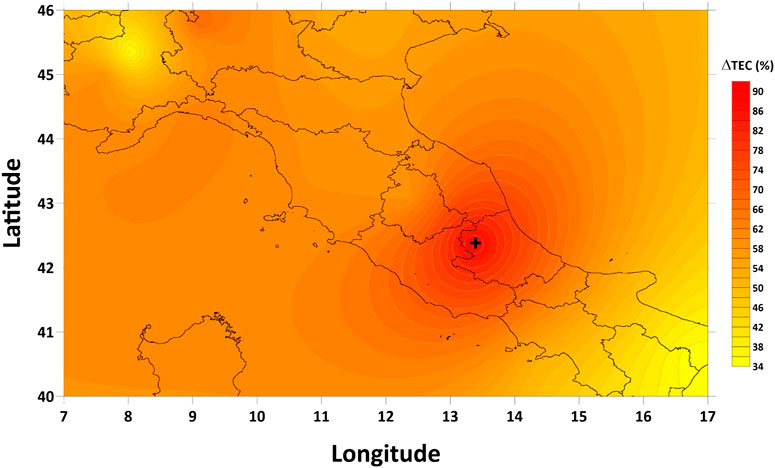
FIGURE 1. Differential map of GPS TEC registered at 22:10 UT on April 4, 2009, 27.3 h before the L’Aquila earthquake.

One can see from the Figure that the deviation is still positive even outside the Italy borders, so it is worth to try the TEC map technology to see how large the positive anomaly is in space. The differential GIM map is presented in Figure 2.

FIGURE 2

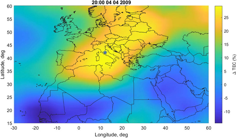
FIGURE 2. Differential GIM map registered at 20:00 UT 03.04.2009, 2 days and 5.5 h before the L’Aquila earthquake.

According to (Pulinets et al., 2004a) the locality of the seismo-ionospheric anomaly could be checked by correlation analysis between different stations in the area situated at different distances from the epicenter. This could be applied to both, the ground based ionosondes and the GNSS receivers. In addition, the variations of the cross-correlation coefficient gives an idea on the time of earthquake because the drop of cross correlation coefficient takes place from 1 to 5 days before the main shock. The cross-correlation coefficient is calculated for the daily arrays of vertical TEC measurements at the selected pairs of receivers for the GPS TEC data and daily arrays of the critical frequency foF2 for selected pairs of ionosondes. Ionosondes selected for the L’Aquila earthquake case study as well as all used GNSS permanent stations are presented on Figure 3.

FIGURE 3

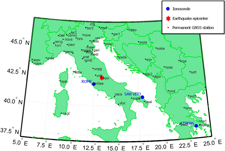
FIGURE 3. Map of the L’Aquila earthquake case area with locations of ionosondes and all used permanent GNSS stations (in a single-station VTEC studies as well as differential TEC map generation).

One more proof that the observed effect is connected with the earthquake preparation is the fact, that for two pairs (Rome-Athens and Rome-San Vito) when the connecting line passes over the earthquake preparation zone, we observe the drop of the cross-correlation coefficient, while for the pair San Vito-Athens, where connecting line is outside the earthquake preparation zone, the drop of cross-correlation coefficient is absent (Tsolis and Xenos, 2010), (Figure 4).

FIGURE 4

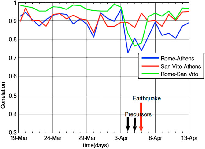
FIGURE 4. Cross-correlation coefficient for three pairs of ionosondes, March-April 2009 (Tsolis and Xenos, 2010), modified.

The similar picture we obtain for the cross-correlation coefficient calculated for the three pairs of the GNSS receivers’ records (Figure 5) (Pulinets and Ouzounov, 2018). The calculation was carried out using data from the aqui (Aquila; aqui (42.368 N, 13.35 E)), ieng (Turin; ieng (45.015 N, 7.639 E)) and prat (Prato; prat (43.886 N, 11.099 E)) receivers. All these receivers were located inside the earthquake preparation zone, the ieng receiver being the farthest from the epicenter. Nevertheless, the reaction of the ionosphere to the earthquake preparation process is seen quite clearly—two days before the earthquake, a significant decrease in the cross-correlation coefficient occurs. The most significant drop in the coefficient is observed between the daily values of the receiver closest to the epicenter and the one farthest from it.

FIGURE 5

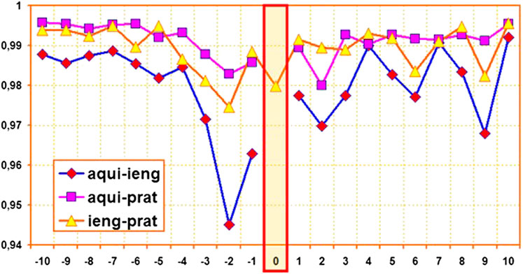
FIGURE 5. Cross-correlation coefficient for three pairs of GPS receivers around the time of L’Aquila earthquake. Time in days around the time of L’Aquila earthquake.

It should be noted that the magnitude of the cross-correlation coefficient drop for GNSS receivers is smaller than for ionosondes what means that the ground based vertical sounding is more sensitive for the correlation analysis.

If the cross-correlation coefficient gives idea on the difference of the seismo-ionospheric effect connected with the distance from epicenter, local spatial scintillation index (LSSI) reflects the variability of the ionosphere within the earthquake preparation zone (Pulinets et al., 2007a).

LSSI demonstrates the scatter of the readings of the GNSS receivers due to mosaic character of gas sources emanating from the system of active faults, its intensity increases as the earthquake approaches (Mareev et al., 2002). The sporadically distributed over the earthquake preparation zone patches of gas emission concentrated mainly around the active parts of tectonic faults provide the local ionization of the near ground layer of atmosphere changing its electric conductivity. These variations are transported by the Global Electric Circuit to the ionosphere and create the effect of spatial scintillation of TEC over the area. Its distribution before the Hector Mine earthquake is shown in (Pulinets and Ouzounov, 2018; Figure 4). The local spatial scintillation index of variability was introduced as the difference between the maximal and minimum values of TEC for every given moment for all the stations under study within the area of interest. The hourly averaged variation of the LSSI index around the time of L’Aquila earthquake is shown in Figure 6.

FIGURE 6

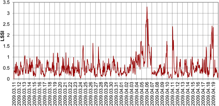
FIGURE 6. Hourly averaged LSSI around the time of L’Aquila earthquake.

Nevertheless, still somebody may demonstrate the doubts, why some variations we associate with the earthquake preparation, and other–with geomagnetic disturbances. In this moment we again should turn to the physical mechanism, which implies that the pre-seismic variations are generated during the nighttime (behind the solar terminator) while the anomalies associated with geomagnetic disturbances are present round the clock and their appearance is connected with the time of geomagnetic disturbance onset (Pulinets and Davidenko, 2018). To notice this difference, we use the special presentation of ionospheric variations called “precursor mask”. Let us look at Figure 7 where from top to bottom are presented the variations of GNSS TEC in percentage for GNSS receiver installed at L’Aquila, variations of the critical frequency foF2 from the Rome ionosonde (also in percentage), and variations of the Global equatorial geomagnetic index Dst also in the 2D colored format similarly to the precursors mask, and then as usual time series graph. The variations of GNSS TEC and Dst presented in the form of mask where the horizontal axis is the day of the year (DOY), vertical axis is the universal Time (UT), and by color scale we demonstrate variations of the parameter under consideration.

FIGURE 7

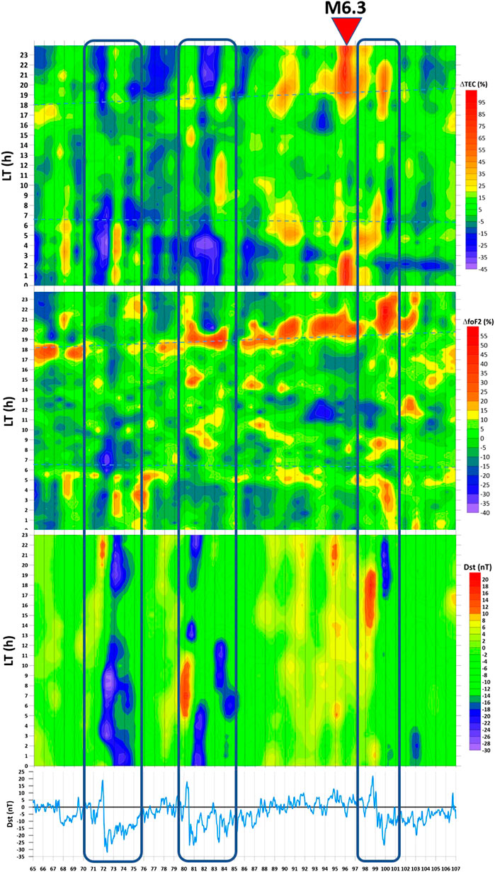
FIGURE 7. From top to bottom: ΔTEC, ΔfoF2, Dst (mask), Dst (time series). In the upper three panels the vertical axis is the Local time, For all panels the horizontal axis is day of the year (DOY). The deviation of the TEC and foF2 in upper two panels is coded by colors and expressed in percentage deviation from the running 15 days median. Dst in the color panel is expressed by colors in nT, In the bottom picture the dst values are shown in the vertical axis.

The periods of small geomagnetic disturbances (first one -31 nT, and other two near -25 nT) are marked at all four plots as black rectangles. Looking at the plots within these rectangles we can mark some effects both in GPS TEC variations and in variations of the critical frequency. They are manifested as vertical blue and red columns (negative and positive deviations). Their appearance depends on the time of geomagnetic disturbance onset, so they are generated both during the day and nighttime. Simultaneously we observe in the first two plots the positive variations which appear only during nighttime, especially few days before the L’Aquila earthquake and one day after (90–97 DOY). Their duration (in local time) is larger for GPS TEC, but the period of their appearance in days before the mainshock is larger in the plot of foF2. Actually, we do not see the emphasized period in post-sunset variations in the ionosonde data, what implies that we possibly observe the pre-reversed enhancement effect (PRE). The only reservation remains that the PRE is essentially the low latitude effect while L’Aquila belongs to the middle latitudes (Eccles et al., 2015).

The most interesting phenomenon, which is obvious at the ΔfoF2 plot is that the pre-sunrize and post sunset anomalies are exactly following the solar terminator. We are in period of equinox when the day length is fast increasing and in the beginning of period of observation (DOY 65–six of March) the time of sunrise is 6:33, and sunset 18:02, and at the end of observation period 17 April the time of sunrise is 6:21, and sunset 19:50. The anomaly in the morning stops earlier than terminator time and in the evening starts earlier than terminator time because of the fact that at altitude of the ionosphere terminator appears earlier than at the ground surface for which we have data for sunrise and sunset time. Lines of terminator time are shown at the ΔfoF2 plot by dashed blue lines. Summarizing: the presented results follow the physical mechanism (Pulinets and Davidenko, 2014; 2018), and ionospheric precursors could be registered by different techniques of the ionosphere monitoring. Using the techniques of data processing (local and GIM mapping, cross-correlation analysis, LSSI index and precursors mask), we were able to uniquely identify the precursors, to find the position of the epicenter of impended earthquakes, and to estimate the time.

To estimate the magnitude, we should have the good estimation of the ionospheric anomaly size which is the same order of magnitude as the size of earthquake preparation zone (Dobrovolsky et al., 1979). Unfortunately, the maps presented in Figures 1, 2 strongly depend on the positions of GPS receivers, quality of interpolation and modeling of GNSS GIM, as well as from the network density and configuration. Additional difficulties for mapping appear if earthquake epicenter is in the ocean. In these circumstances, we should have the direct measurements of the ionospheric anomaly dimensions that could be provided only by topside sounding as it was done for Irpinia M6.9 earthquake on November 23, 1980 in Italy (Pulinets et al., 2007b). This technology is demonstrated in Figure 8 presenting the variations of critical frequency foF2 deviation from undisturbed state while satellite passing over the seismo-ionospheric anomaly. Estimating anomaly radius as 900 km, the magnitude M would be M = [log (900)]/0.43 = 6.9.

FIGURE 8

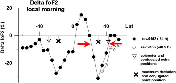
FIGURE 8. Deviation of the critical frequency foF2 along the orbit of Intercosmos-19 satellite.

Discussion

The presented examples reveal the variety of techniques for the reliable identification of the ionospheric precursors, only for one event–the L’Aquila earthquake. Then a natural question arise: how stable these characteristic features of the ionospheric precursors are. Whether we will observe similar results worldwide, and not only in quiet geomagnetic conditions, but also in the disturbed cases?

The statistical study of the precursor mask stability was provided for Greece and Italy areas (Davidenko and Pulinets, 2019). The left panel of Figure 9 shows an averaged mask for earthquakes with M ≥ 6 in Greece for period 2006–2018, and the right panel–the mask for the critical frequency variation for the same interval of time. GNSS TEC data were collected from receiver located in Athens, while vertical sounding data from two ionosondes situated in Athens and Sofia.

FIGURE 9

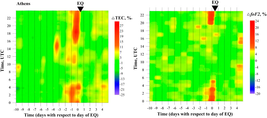
FIGURE 9. Left panel–the precursor mask derived from the data of GPS TEC receiver in Rome; right panel–the precursors mask for critical frequency foF2 deviations derived from the data of the Rome ionospheric station of vertical sounding (Davidenko and Pulinets, 2019).

As we observed in Figure 7 the GNSS TEC anomalies last longer (within the day) than the critical frequency ones.

The situation in Italy is more complex and probably due to the difference in geological structure of the Apennines peninsula (Meletti et al., 2000). We observe a similar precursor mask structure for the northern and central Italy, and opposite sign of the pre-seismic anomaly (negative deviations) for the southern Italy except Sicily. This issue is the subject of future research. For a clarity and consistence of the discussion we demonstrate here in Figure 10 the GNSS TEC (left panel) and critical frequency (right panel) masks for the northern part of Italy. Taking into account that the seismic activity in Italy is generally lower than in Greece, we set the lower magnitude threshold −5.4. On the other hand, the period of ionosphere data availability is even longer than in Greece: 1962–2017 for the Rome ionosonde (used for earthquakes in the range of 300 km in northern direction from Rome) and 1997–2017 for Medicine GNSS receiver (used for earthquakes with M ≥ 6 in northern Italy). One can clearly see the high similarity the GNSS TEC and critical frequency foF2 masks regardless the different intervals of integration what confirms the high stability of the observed effect for multi-year observations.

FIGURE 10

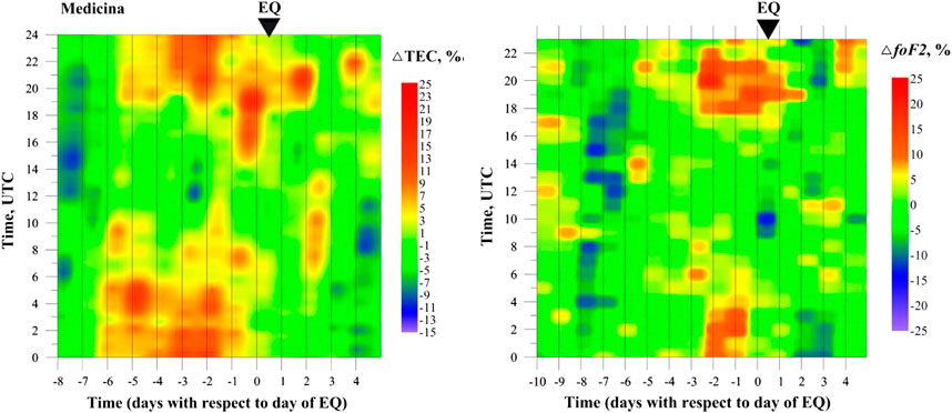
FIGURE 10. Left panel–the precursor mask derived from the data of GPS TEC receiver in Medicine; right panel–the precursors mask for critical frequency foF2 deviations derived from the data of the Rome ionospheric station of vertical sounding (Davidenko and Pulinets, 2019).

In Italy–similarly to the L’Aquila case–precursory structure is observed during several consecutive days whereas in Greece precursor is observed only during one day.

It is interesting to note that precursors identification using the mask technology is possible not only in quiet geomagnetic conditions with small disturbances but also during strong geomagnetic storms and high geomagnetic activity. In Figure 11 one can see the precursor mask for the case of Hector Mine M7.1 earthquake on October 16, 1999 in California.

FIGURE 11

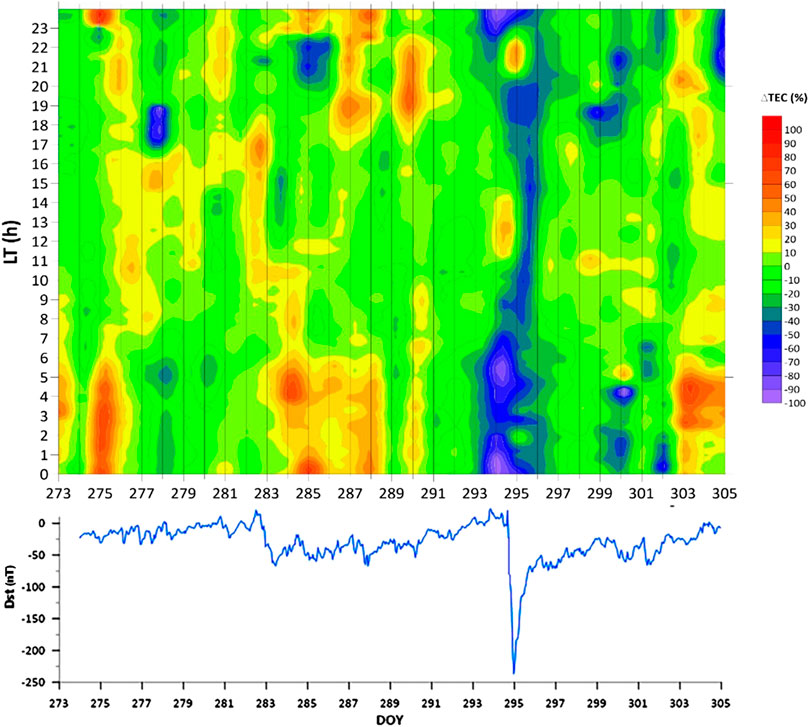
FIGURE 11. Upper panel GPS TEC mask for gol2 GPS receiver (35.4 N; 243.1 W), Hector Mine earthquake 289 DOY, lower panel global equatorial geomagnetic index Dst.

The nighttime positive anomalies are clearly visible from one to four days before the Hector mine earthquake, as well as a thick blue negative bar during strong geomagnetic storm with −250 nT peak value.

Having the technology of ionospheric precursor identification, we propose the system for automatic data processing, interpretation, precursors identification and possible earthquake forecast.

Implementation

The developed algorithm presented in Figure 12 shows the sequence of operations in the corresponded branches of the data processing. The implementation of these operations leads to detection of the anomaly which corresponds with seismo-ionospheric coupling mechanism triggered during an earthquake’s preparation period.

FIGURE 12

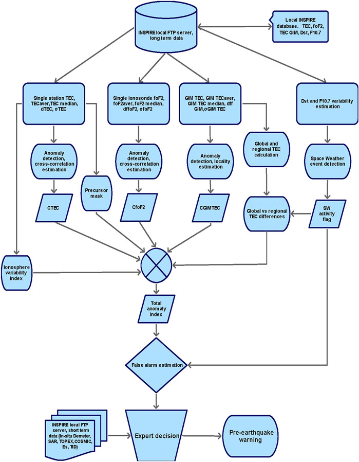
FIGURE 12. The algorithm based on the sequence of operations in the corresponded branches of the data processing.

In order to give comprehensive prediction, specifications the multi-parameter and systematic approach of different databases described above can be established.

The databases involve a range of ionospheric, Space Weather and some additional observations and products. The ionospheric parameters database includes ionosonde measurements of the critical frequency foF2, Global VTEC maps (GIMs) and local VTEC values calculated for each station. The Space Weather part includes series of solar and geomagnetic activity parameters–F10.7 solar flux and Dst indices. The additional database include short-time observations performed with a range of different instruments (RO electron density profiles from COSMIC observations, in-situ observations from Demeter mission, altimeter VTEC observations, InSAR co-seismic displacement data).

The further processing is divided in separate branches: the local TEC anomaly processing, the local foF2 anomaly processing, the global TEC processing, and Space Weather processing.

The local TEC processor calculates the TEC anomaly and TEC variability index based on the VTED values observed with the selected stations. This branch incorporates also building the TEC precursor mask. The mask is a matrix A_ij, where i is the TEC sample in a day and j corresponds with subsequent days preceding the earthquake. The precursor pattern matrix created using statistical data processing and image recognizing techniques (on the base of a-priori geological information/maps) in the given region is compared with the current measurements.

The foF2 processor branch, similarly to the local TEC branch, calculates the foF2 anomaly and variation index, by calculating the running average of the parameter, differential foF2 and cross-correlation between two sets of the diurnal variation (same as) of the critical frequency values from two spaced ionosondes.

The global TEC processing branch calculates the 2D TEC anomaly as well as the TEC anomaly location together with the Global Electron Content (GEC) and Regional Electron Content (REC).

The Space Weather branch processes the F10.7 and Dst indices series to obtain disturbances flags, by a proper leveling and generating flags, when index exceeds the threshold.

In the next step, the synergic analyzer collects previously obtained parameters together with other, non-ionospheric seismic information. The synergic analyzer checks the temporal sequence and spatio-temporal synchronization of the detected anomalies and compares to the model pattern. Also very important is the step of false alarm detection, where the false alarm flag against the total anomaly index is provided.

The final step involves the experts’ decision, during which the seismologists and geophysicists examines the detected anomalies of ionospheric and non-ionospheric origin, their spatial and temporal characteristics. Also the role of an expert is to make a decision about the pre-seismic warning.

Earthquake preparation process is a complex open system including inter-geosphere interactions; therefore, we should control all the system at different levels, starting from underground through atmosphere up to the ionosphere and magnetosphere. One of the main important topics is the adequate real time data acquisition with time delay no more than 1 h including also validation, authorization and unification data derived from different instruments and databases. In addition, the detailed calibration procedure for determination of set of meridian environmental condition for selected territories of seismoactive zone can be established.

Indication of New Experimental Investigations and Observations

The global and local networks of ground-based GNSS-receivers give an unique chance for monitoring of the near Earth’s environment conditions in a global scale. Nowadays more than 5,000 permanent ground-based GNSS stations provide measurements to the community. Further evolution relates with increasement of the number of GNSS stations and modernization of receivers with ability to track signals from various systems. The development of the European Galileo system, the Russian GLONASS and the Chinese BeiDou/COMPASS system will improve the monitoring and diagnostics of the seismic origin TEC perturbations. Furthermore, microwave and HF radars diagnostics scatterometers, altimeters for topography, GNSS satellite receivers for reflectometry, and imaging radars SAR together with space plasma diagnostics in situ can be an excellent set for such new diagnostics campaign.

The recently launched Jason-3 mission continues the core satellite altimetry measurements. Its payload consists of the same core instruments as Jason-2: a Poseidon class Ku/C-band radar altimeter to provide the primary ranging measurement, a nadir-looking three frequency (18.7, 23.8, and 34.0 GHz) microwave radiometer (as flown on Jason-2), along with a POD (Precise Orbit Determination) package consisting of a GPS (Global Positioning System) receiver, DORIS (Doppler Orbitography and Radiopositioning Integrated by Satellite), and a LRA (Laser Retroreflector Array), as flown on prior Jason series missions. The satellite is placed on a circular non Sun synchronous orbit with altitude of 1,336 km and inclination 66.038°.

To support the ionospheric precursors monitoring the additional parameters provided by satellite systems could be useful, namely, the mechanical deformations and thermal pre-earthquake anomalies. The fast developing SENTINEL program gives the perfect opportunities for these additions. The SENTINEL-1 Satellite Constellation consist of two satellites: SENTINEL-1A and SENTINEL-1B launched in 2014 and 2016 respectively. Both of them have a single C-band synthetic-aperture radar (C-SAR) which is able to provide the high resolution SAR interferometry to detect land deformation before and after earthquakes. The SENTINEL-3 satellite constellation: SENTINEL-3A and SENTINAL-3B were launched in 2006 and 2018 respectively have SLSTR (Sea and Land Surface Temperature Radiometer) to measure the surface ocean and land temperature what will permit to detect the thermal anomalies before earthquakes, and SRAL (Synthetic Aperture Radar Altimeter) also could be used for SAR interferometry. The new ESA’s Swarm mission was launched on November 2013. The mission is a constellation of the three identical satellites Alpha, Bravo and Charlie. Two of them fly in a tandem with one degree separation at the altitude of 460 km, the third one is placed higher, at 510 km. The latter allows comparison of measurements from identical instruments at different altitudes and in the different longitudinal sectors. The satellite payload has Langmuir Probe instrument for the in situ plasma density measurements and GPS receiver for POD measurements. Near polar orbits are required to provide a global coverage—multi-point measurements at global and regional scales, as required for spatial and temporal sampling of the fields, imply the deployment of a constellation. The main Swarm instrument is the Vector Field Magnetometer. It performs high-precision measurements of the magnitude and direction of the magnetic field. Together with the Absolute Scalar Magnetometer it is a very sensitive instrument to study tiny magnetic signatures from ground. Also the ESA-funded project SAFE (SwArm For Earthquake study) devoted to the pre-seismic effects and based on the Swarm magnetometric measurement data is worth mentioning. This project is coordinated by the INGV (Italy). The investigations are based on the data collected from satellites and from ground-based instruments, the phase preceding the great earthquakes with the aim to identify any electromagnetic signal from space.

The topside ionosphere sounding based on LEO nano satellite cluster located in different local time sectors, as well as ground based ionosonde network, can give an opportunity for detailed diagnostics of morphology and dynamic of large and small scales ionosphere structures. New 3D measurements of the electric and magnetic fields particles diagnostics located on LEO nano satellites should bring the additional improvement of the atmosphere-ionosphere-magnetosphere coupling processes monitoring.

Finally, the radio-occultation inversion techniques for ionospheric tomography, already improved in the last years, are able to provide worldwide distributed electron density profiles over the land and seas in a very efficient way. The coverage is still increasing with the launch of COSMIC constellation, and with the already launched COSMIC-2 constellation and Chinese Feng Yun 3C satellite constellations.

The new follow-on mission to the FORMOSAT-3/COSMIC is the FORMOSAT-7/COSMIC-2. It is a constellation of six remote sensing microsatellites able to provide new data for ionosphere research. The goal is to collect a large amount of atmospheric and ionospheric data. The new constellation provides improved performance and a significant increase in number of measurements. Formosat-7 established operational Mission of near real-numerical weather prediction that collects few thousands of the electron density profiles per day. The satellite RO receivers have GPS, GALILEO and GLONASS tracking capability. COSMIC-2 also has RF Beacon transmitters and Velocity, Ion Density, and Irregularities (VIDI) instruments—plasma probes. The launch of six satellites of the low inclination constellation took place on June 25, 2019. The constellation of six satellites is planned to reach their operational orbits at 24° inclination, which will enhance observations in the equatorial region, on first quarter of 2021.

So, it is possible to conclude that a unique opportunity to study the seismo-ionospheric effects with an unprecedentable number of ground and space base measurements, will exist in the near future.

Obviously, we are living now in the epoch when the amount of the multi-instrumental ground- and space-based measurements is extremely high and it increases progressively. But only specific earthquake-oriented satellite mission can bring a clue on how to match all these new and wide datasets to a consitent interpretation of the Lithosphere-Atmosphere-Ionosphere Coupled System.

Indication of the Possible New Services Based on the Proposed

The technology of ionosphere monitoring described in the previous chapters, combined with the ground support and other (not ionospheric) precursors monitoring, are able to provide the reliable information on the main parameters necessary for the short-term earthquake forecast: i.e., epicenter position, magnitude and time of the impending seismic event. The service of the short-term forecast could be proposed in conditions that the corresponding infrastructure will be created for the continuous real monitoring of indicated parameters of ionosphere and magnetosphere and described in terms of atmospheric parameters.

As a limited option for some areas with extended network of ground-based GNSS receivers such as Japan, California, Europe such service can be proposed now, but again this service should be organized through a proper infrastructure of data-centers and analysis centers with corresponding connection with decision makers in governmental municipal institutions.

Special service of the short-term warning can be created for the users of mobile devices in the earthquake-prone areas.

Taking into account that the model has a worldwide scope in terms of the atmosphere-ionosphere coupling, the other natural and anthropogenic hazards could be monitored using the same technology–like the dust and sand storms, hurricanes, volcano eruptions and the ash clouds tracking, radioactive pollution (for example, emergencies at the atomic power plants, such as Three-Mile Island, Chernobyl or Fukushima). Also the nuclear weapon tests could be monitored. The both tests in the Northern Korea were registered in the ionosphere using the GIM maps.

The specialized space mission should be initiated to make the proposed project live, real, and working in real time.

Data Availability Statement

The datasets presented in this article are not readily available because The dataset is based of LAIC model by Sergey Pulinets. Requests to access the datasets should be directed to pulse1549@gmail.com.

Author Contributions

SP, AK, IZ, and IC contributed the methodology of the study; SP, AK, MH-P, IC, IZ, DD, HR, KK, PF, AF, AR, and PB contributed in the data acquisition and dataset building; IC, IZ, DD, KK, PF, LB. AF, AR, and PB contributed in the data analysis; SP, AK, MH-P, IC, IZ, and KK contributed in the manuscript preparation, AK and SM were responsible for the project supervising.

Funding

In years 2014–2016 works were supported by the ESA Project “INSPIRE, ionosphere Sounding for Pre-seismic anomalies Identification Research (INSPIRE)” nr 4000,111,456/14/NL/MV. The work is supported by the National Center for Research and Development, Poland, through Grant ARTEMIS (decision no. DWM/PL-CHN/97/2019, WPC1/ARTEMIS/2019); The authors thank also the Ministry of Science and Higher Education (MSHE), Poland for granting funds for the Polish contribution to the International LOFAR Telescope “(MSHE decision no. DIR/WK/2016/2017/05–1)” and for maintenance of the LOFAR PL-612 Baldy (MSHE decisions: no. 59/E-383/SPUB/SP/2019.1). This work is supported by the National Science Centre, Poland, through Grants 2017/25/B/ST10/00479 and 2017/27/B/ST10/02190.

Conflict of Interest

The authors declare that the research was conducted in the absence of any commercial or financial relationships that could be construed as a potential conflict of interest.

Acknowledgments

The work was based on the data provided by the IGS, EPN, UNAVCO, GIRO, DEMETER, FORMOSAT-3/COMIC-7 and SWARM services.

References

Blaunstein, N., and Hayakawa, M. (2009). Short-term ionospheric precursors of earthquakes using vertical and oblique ionosondes. Phys. Chem. Earth, Parts A/B/C 34, 496–507. doi:10.1016/j.pce.2008.07.002

CrossRef Full Text | Google Scholar

Bogdanov, V. V., Kaisin, A. V., Pavlov, A. V., Polyukhova, A. L., and Meister, C.-V. (2017). Anomalous behavior of ionospheric parameters above the kamchatka peninsula before and during seismic activity. Phys. Chem. Earth, Parts A/B/C 98, 154–160. doi:10.1016/j.pce.2016.04.002

CrossRef Full Text | Google Scholar

Chang, F. Y., Liu, J. Y., Chang, L. C., Lin, C.-H., and Chen, C.-H. (2015). Three-dimensional electron density along the WSA and MSNA latitudes probed by FORMOSAT-3/COSMIC coupling of the high and mid latitude ionosphere and its relation to geospace dynamics space science. Earth, Planets and Space 67 (1). doi:10.1186/s40623-015-0326-8

CrossRef Full Text | Google Scholar

Datchenko, E. A., Ulomov, V. I., and Chernyakova, C. P. (1972). Electron density anomalies as the possible precursor of tashkent earthquake. Dokl. Uzbek. Acad. Sci. 12, 30–32.

Google Scholar

Dautermann, T., Calais, E., Haase, J., and Garrison, J. (2007). Investigation of ionospheric electron content variations before earthquakes in southern California, 2003-2004. J. Geophys. Res. 112, B02106. doi:10.1029/2006JB00444710.1029/2006jb004447

CrossRef Full Text | Google Scholar

Davidenko, D. V., and Pulinets, S. A. (2019). Deterministic variability of the ionosphere on the eve of strong (M ≥ 6) earthquakes in the regions of Greece and Italy according to long-term measurements data. Geomagn. Aeron. 59 (4), 493–508. doi:10.1134/S001679321904008X

CrossRef Full Text | Google Scholar

Davies, K., and Baker, D. M. (1965). Ionospheric effects observed around the time of the Alaskan earthquake of March 28, 1964. J. Geophys. Res. 70, 2251–2253. doi:10.1029/jz070i009p02251

CrossRef Full Text | Google Scholar

Dobrovolsky, I. P., Zubkov, S. I., and Miachkin, V. I. (1979). Estimation of the size of earthquake preparation zones. Pageoph 117, 1025–1044. doi:10.1007/bf00876083

CrossRef Full Text | Google Scholar

Eccles, J. V., St. Maurice, J. P., and Schunk, R. W. (2015). Mechanisms underlying the prereversal enhancement of the vertical plasma drift in the low‐latitude ionosphere. J. Geophys. Res. Space Phys. 120, 4950–4970. doi:10.1002/2014JA020664

CrossRef Full Text | Google Scholar

Hirooka, S., Hattori, K., Nishihashi, M., and Takeda, T. (2011). Neural network based tomographic approach to detect earthquake-related ionospheric anomalies. Nat. Hazards Earth Syst. Sci. 11, 2341–2353. doi:10.5194/nhess-11-2341-2011

CrossRef Full Text | Google Scholar

Kon, S., Nishihashi, M., and Hattori, K. (2011). Ionospheric anomalies possibly associated with M⩾6.0 earthquakes in the Japan area during 1998-2010: case studies and statistical study. J. Asian Earth Sci. 41 (4), 410–420. doi:10.1016/j.jseaes.2010.10.005

CrossRef Full Text | Google Scholar

Krankowski, A., Zakharenkova, I. E., and Shagimuratov, I. I. (2006). Response of the ionosphere to the baltic sea earthquake of 21 september 2004. Acta Geophys. 54, 90–101. doi:10.2478/s11600-006-0008-9

CrossRef Full Text | Google Scholar

Li, M., and Parrot, M. (2013). Statistical analysis of an ionospheric parameter as a base for earthquake prediction. J. Geophys. Res. Space Phys. 118 (A6), 3731–3739. doi:10.1002/jgra.50313

CrossRef Full Text | Google Scholar

Liu, J.-Y., and Chao, C.-K. (2017). An observing system simulation experiment for FORMOSAT-5/AIP detecting seismo-ionospheric precursors. Terr. Atmos. Ocean. Sci. 28, 117–127. doi:10.3319/TAO.2016.07.18.01(EOF5)

CrossRef Full Text | Google Scholar

Liu, J. Y., Chen, Y. I., Chen, C. H., Liu, C. Y., Chen, C. Y., Nishihashi, M., et al. (2009). Seismoionospheric GPS total electron content anomalies observed before the 12 May 2008Mw7.9 Wenchuan earthquake. J. Geophys. Res. 114 (A04320). doi:10.1029/2008JA013698

CrossRef Full Text | Google Scholar

Liu, J. Y., Chen, Y. I., Chuo, Y. J., and Chen, C. S. (2006). A statistical investigation of preearthquake ionospheric anomaly. J. Geophys. Res. 111 (A05304). doi:10.1029/2005JA011333

CrossRef Full Text | Google Scholar

Liu, J. Y., Chuo, Y. J., Shan, S. J., Tsai, Y. B., Chen, Y. I., Pulinets, S. A., et al. (2004). Pre-earthquake ionospheric anomalies registered by continuous GPS TEC measurements. Ann. Geophys. 22 (5), 1585–1593. doi:10.5194/angeo-22-1585-2004

CrossRef Full Text | Google Scholar

Liu, J.‐Y., Hattori, K., and Chen, Y. (2018). “Application of total electron content derived from the Global Navigation Satellite System for detecting earthquake precursors,” in In pre‐earthquake processes: a multidisciplinary approach to earthquake prediction studies (geophysical monograph 234). Editors D. Ouzounov, S. Pulinets, K. Hattori, and P. Taylor (Washington, DC: American Geophysical UnionJohn Wiley and Sons, Inc.), 305–318.

Google Scholar

Mareev, E. A., Iudin, D. I., and Molchanov, O. A. (2002). “Mosaic source of internal gravity waves associated with seismic activity,” in In seismo-electromagnetics: lithosphere-atmosphere-ionosphere coupling. Editors M. Hayakawa, and O. A. Molchanov (Tokyo, Japan: TERRAPUB), 335–342.

Google Scholar

Meletti, C., Patacca, E., and Scandone, P. (2000). Construction of a seismotectonic model: the case of Italy. Pure Appl. Geophys. 157, 11–35. doi:10.1007/pl00001089

CrossRef Full Text | Google Scholar

Ouzounov, D., Pulinets, S., Hattori, K., and Taylor, P. (2018). Pre‐earthquake processes: a multidisciplinary approach to earthquake prediction studies. in Geophysical monograph series, No 234. Hoboken, NJ: American Geophysical UnionAGU/Wiley. doi:10.1002/9781119156949

CrossRef Full Text

Parrot, M., and Li, M. (2018). “Statistical analysis of the ionospheric density recorded by DEMETER during seismic activity,” in In pre‐earthquake processes: a multidisciplinary approach to earthquake prediction studies (geophysical monograph 234). Editors D. Ouzounov, S. Pulinets, K. Hattori, and P. Taylor (Washington, DC: American Geophysical UnionJohn Wiley and Sons, Inc.), 319–330.

CrossRef Full Text | Google Scholar

Pulinets, S. A., Biagi, P., Tramutoli, V., Legen’ka, A. D., and Depuev, V. K. (2007). Irpinia earthquake 23 November 1980 – lesson from Nature revealed by joint data analysis. Ann. Geophys. 50 (1), 61–78. doi:10.4401/ag-3087

Google Scholar

Pulinets, S. A., Bondur, V. G., Tsidilina, M. N., and Gaponova, M. V. (2010). Verification of the concept of seismoionospheric coupling under quiet heliogeomagnetic conditions, using the Wenchuan (China) earthquake of May 12, 2008, as an example. Geomagn. Aeron. 50, 231–242. doi:10.1134/s0016793210020118

CrossRef Full Text | Google Scholar

Pulinets, S. A., Davidenko, D. V., and Budnikov, P. A. (2021). Cognitive recognition of the ionospheric precursors of earthquakes. Geomagnetism and Aeronomy 61, 39–50. doi:10.4401/ag-3087

CrossRef Full Text | Google Scholar

Pulinets, S. A., and Davidenko, D. V. (2018). The nocturnal positive ionospheric anomaly of electron density as a short-term earthquake precursor and the possible physical mechanism of its formation. Geomagn. Aeron. 58, 559–570. doi:10.1134/s0016793218040126

CrossRef Full Text | Google Scholar

Pulinets, S. A., Gaivoronska, T. B., Leyva Contreras, A., and Ciraolo, L. (2004a). Correlation analysis technique revealing ionospheric precursors of earthquakes. Nat. Hazards Earth Syst. Sci. 4, 697–702. doi:10.5194/nhess-4-697-2004

CrossRef Full Text | Google Scholar

Pulinets, S. A., Kotsarenko, A. N., Ciraolo, L., and Pulinets, I. A. (2007a). Special case of ionospheric day-to-day variability associated with earthquake preparation. Adv. Space Res. 39 (5), 970–977. doi:10.1016/j.asr.2006.04.032

CrossRef Full Text | Google Scholar

Pulinets, S. A., Legen’ka, A. D., Gaivoronskaya, T. V., and Depuev, V. K. (2003). Main phenomenological features of ionospheric precursors of strong earthquakes. J. Atmos. Solar-Terrestrial Phys. 65, 1337–1347. doi:10.1016/j.jastp.2003.07.011

CrossRef Full Text | Google Scholar

Pulinets, S. A., and Legen’ka, A. D. (2003). Spatial-temporal characteristics of large scale distributions of electron density observed in the ionospheric F-region before strong earthquakes. Cosmic Res. 41 (3), 221–230. doi:10.1023/a:1024046814173

CrossRef Full Text | Google Scholar

Pulinets, S. A., Liu, J. Y., and Safronova, I. A. (2004). Interpretation of a statistical analysis of variations in the foF2 critical frequency before earthquakes based on data from Chung-Li ionospheric station (Taiwan). Geomagnetism and Aeronomy 44 (1), 102–106.

Google Scholar

Pulinets, S. A., Ouzounov, D. P., Karelin, A. V., and Davidenko, D. V. (2015). Physical bases of the generation of short-term earthquake precursors: a complex model of ionization-induced geophysical processes in the lithosphere–atmosphere–ionosphere–magnetosphere system. Geomagnetism and Aeronomy 55 (4), 540–558. doi:10.1134/s0016793215040131

CrossRef Full Text | Google Scholar

Pulinets, S. A., Romanov, A. A., Urlichich, Y. M., Romanov, A. A., Doda, L. N., and Ouzounov, D. (2009). The first results of the pilot project on complex diagnosing earthquake precursors on sakhalin. Geomagn. Aeron. 49 (1), 115–123. doi:10.1134/s0016793209010162

CrossRef Full Text | Google Scholar

Pulinets, S. A. (1998). Strong earthquake prediction possibility with the help of topside sounding from satellites. Adv. Space Res. 21 (3), 455–458. doi:10.1016/s0273-1177(97)00880-6

CrossRef Full Text | Google Scholar

Pulinets, S., and Boyarchuk, K. (2004). Ionospheric precursors of earthquakes. Mexico, Springer.

Pulinets, S., and Davidenko, D. (2014). Ionospheric precursors of earthquakes and global electric circuit. Adv. Space Res. 53, 709–723. doi:10.1016/j.asr.2013.12.035

CrossRef Full Text | Google Scholar

Pulinets, S., Ouzounov, D., Karelin, A., and Davidenko, D. (2018). ““Lithosphere–Atmosphere–Ionosphere–Magnetosphere coupling – a concept for pre‐earthquake signals generation,” in In pre‐earthquake processes: a multidisciplinary approach to earthquake prediction studies (geophysical monograph 234). Editors D. Ouzounov, S. Pulinets, K. Hattori, and P. Taylor (Washington, DCHoboken, NJ: American Geophysical UnionJohn Wiley and Sons, Inc.), 79–98.

Google Scholar

Pulinets, S., and Ouzounov, D. (2018). The possibility of earthquake forecasting. Learning from nature. Bristol: IOP Publishing. doi:10.1088/978-0-7503-1248-6

CrossRef Full Text | Google Scholar

Romanov, A. A., Romanov, A. A., Trusov, S. V., and Urlichich, Y. M. (2013). Satellite tomography of the ionosphere. Moscow: Fizmatlit publ

Rozhnoi, A., Solovieva, M., Molchanov, O., Schwingenschuh, K., Boudjada, M., Biagi, P. F., et al. (2009). Anomalies in VLF radio signals prior the Abruzzo earthquake (M=6.3) on 6 April 2009. Nat. Hazards Earth Syst. Sci. 9, 1727–1732. doi:10.5194/nhess-9-1727-2009

CrossRef Full Text | Google Scholar

Thomas, J. N., Love, J. J., Komjathy, A., Verkhoglyadova, O. P., Butala, M., and Rivera, N. (2012). On the reported ionospheric precursor of the 1999 hector mine, California earthquake. Geophys. Res. Lett. 39, L06302. doi:10.1029/2012GL051022

CrossRef Full Text | Google Scholar

Tsolis, G. S., and Xenos, T. D. (2010). A qualitative study of the seismo-ionospheric precursors prior to the 6 April 2009 earthquake in L’Aquila, Italy. Nat. Hazards Earth Syst. Sci. 10, 133–137. doi:10.5194/nhess-10-133-2010

CrossRef Full Text | Google Scholar