Comparing Greenland Ice Sheet Melt Variability From Different Satellite Passive Microwave Remote Sensing Products Over a Common 5-year Record

Introduction

During the past two decades, contributions to global sea level rise from the Greenland Ice Sheet (GrIS) have increased more than any other source (Chen et al., 2017). This increased mass loss has resulted in large part from a disproportionate decrease in the ice sheet surface mass balance (Enderlin et al., 2014; van den Broeke et al., 2016). Ice sheet surface melt and runoff has increased sharply since the early 1990s (van den Broeke et al., 2016; Fettweis et al., 2017). Ice sheet record melt extremes have occurred no fewer than four times since 2000 alone (Nghiem, 2005; Mote, 2007; Tedesco et al., 2011; Tedesco et al., 2013), and most recently during the summer of 2019 (Tedesco and Fettweis, 2020). Consequently, surface melting of the GrIS is a research topic with increasing significance and global implications.

Observationally constrained surface melting at the ice sheet scale can only be obtained through satellite remote sensing. Because the dielectric constant of water is much larger than the dielectric constant of ice (∼35 for water compared to 3.2 for ice at 20 GHz (Foster et al., 1984)), the presence of water in the snowpack raises the dielectric constant of the medium. This has the effect of increasing the electromagnetic (EM) energy absorptivity of the medium and, following Kirchoff’s law, also the EM emission. The presence of liquid water in the snowpack therefore substantially alters the surface microwave emissions; an effect which is enhanced at frequencies above 10 GHz (Ulaby et al., 1986). Similar frequency microwave brightness temperature (Tb) retrievals are readily available from polar-orbiting operational global satellites that enable effective monitoring of surface melt dynamics over the GrIS.

Polar-orbiting spaceborne microwave radiometers have operated since the late 1970s, providing consistent and relatively well calibrated Tb retrievals at frequencies (19–37 GHz) sensitive to the large surface dielectric changes that occur in response to melt-induced increases in snowpack liquid water abundance. The Tb retrievals at these microwave frequencies are insensitive to solar illumination, cloud and atmospheric aerosol contamination, enabling comprehensive coverage and frequent (∼daily) sampling of GrIS melt dynamics, but at relatively coarse (∼25 km) spatial resolution. A number of different satellite microwave-based melt products have been developed over the GrIS, involving different sensors, Tb frequencies and polarizations, and retrieval algorithms with varying levels of performance (Mote, (2007); Tedesco, 2007; Tedesco, 2014; Kim et al., 2017). These products have been used for a range of applications, including quantifying long-term environmental trends in GrIS melt conditions (e.g. Abdalati and Steffen, 1997; Fettweis et al., 2007; Tedesco, 2007) and identifying anomalous melt events (Mote, (2007); Tedesco et al., 2013; Tedesco and Fettweis, 2020). Microwave melt products have also been used as a unique, observation-based validation metric for regional climate models (Fettweis et al., 2005; Fettweis et al., 2006; Fettweis et al., 2011).

A number of different approaches have been developed to interpret measured brightness temperatures as a binary melt/no melt field across the ice surface. Many techniques rely on the determination of a Tb threshold; whereby, Tb retrievals exceeding this threshold are classified as melt. While the foundational data upon which the melt products are derived is largely consistent, the relatively large diversity of approaches used to determine melt conditions implies that the melt determination from any single method contains a degree of uncertainty. While some studies have compared selected melt products (e.g. Tedesco, 2007; Fettweis et al., 2011), the degree of agreement between different published methods remains unclear. Considering the value of satellite microwave-based melt products for monitoring GrIS melt conditions, determining long-term environmental trends, and as observational benchmarks for validating regional climate models, an updated assessment of available products is warranted.

In this study, we performed a comparison of six microwave melt products over the GrIS and spanning a common 5-year study period (2003–2007). Five of the melt products selected are relatively well documented and established from the literature. A sixth algorithm, developed to be integrated into an existing global freeze-thaw Earth System Data Record (Kim et al., 2017), is introduced and included in the comparison. The melt products were compared to data collected by a GrIS network of on-ice automatic weather stations (AWS) to determine their agreement with in situ melt events indicated from temperature measurements. An intercomparison was also performed to assess spatial and temporal agreement between the different satellite derived melt products, which may prove especially useful to end users seeking to use the these products to inform cryosphere and climate change research.

Methods

Existing Microwave Melt Products

Five published melt products were selected for the comparison, each of which was developed specifically for application to the GrIS. To maintain consistency with publicly available products (e.g. Mote and Anderson, 1995), which have been masked following (Friedl et al., 2002), the same ice mask was applied to all products here. The melt products evaluated in this study are summarized in Table 1.

TABLE 1

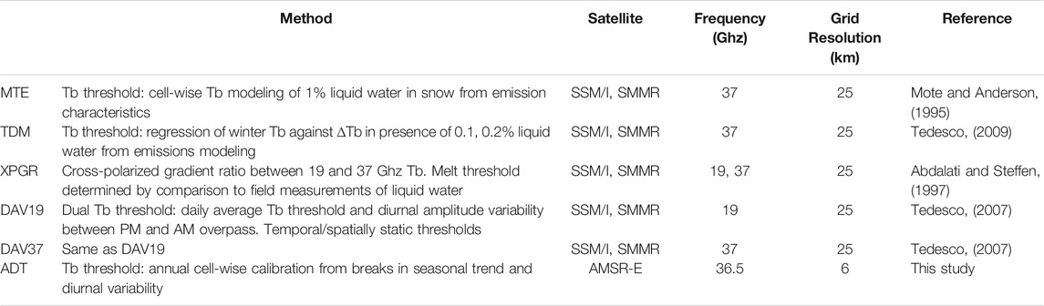
TABLE 1. Summary of tested microwave-based surface melt products.

Mote and Anderson (1995) Emission Modeling-Based Melt Product (MTE)

Mote and Anderson, (1995); Mote, (2007) determined a Tb threshold distinguishing between frozen and melted snow conditions using a microwave emissions modeling approach. With scattering coefficients inverted from winter Tb reference measurements and assumed snow grain size, snow density, and snowpack temperature over the GrIS, Tb thresholds were computed for a modeled snowpack with 1% liquid water content. These thresholds were compared to 37 GHz, horizontally (H) polarized Tb retrievals from SSM/I (Special Sensor Microwave/Imager) and SMMR (Scanning Multichannel Microwave Radiometer) sensor records to determine melt conditions. The melt product is freely available from NSIDC (https://nsidc.org/data/nsidc-0533/versions/1), and is hereafter referred to as MTE.

Tedesco (2014) Emission Modeling-Based Melt Product (TDM)

Similar to Mote and Anderson (1995), the melt product described in Tedesco (2014), and based on initial development in Tedesco (2009) and Tedesco et al. (2013), defines a Tb threshold from microwave emissions modeling. The change in Tb (∆Tb) during the transition to wetted conditions is simulated for a range of initial dry snow (e.g. winter) Tb values. Wetted conditions are defined from a reference 5 cm snowpack with 0.1–0.2% liquid water content. The winter Tb-specific offset is then used to define spatially variable Tb threshold values across the GrIS. Melt days are determined when the satellite observed (SSM/I or SMMR) 37H GHz Tb retrieval exceeds the threshold. The resulting melt product is publicly available (http://www.cryocity.org/data.html) and is hereafter referred to as TDM.

XPGR

Abdalati and Steffen (1995), Abdalati and Steffen, (1997) exploited the frequency- and polarization-dependence of emission sensitivity to liquid water to define melt conditions based on exceedance of a threshold value in the cross-polarized gradient ratio of 19 and 37 GHz, horizontally (H) and vertically (V) polarized Tb retrievals:

$XPGR=\frac{T_b\left(19H\right)-T_b\left(37V\right)}{T_b\left(19H\right)+T_b\left(37V\right)}(1)$

Here we apply the same XPGR algorithm to SSM/I brightness temperatures and use the same adaptive threshold values for the F11 and F13 satellite platforms (XPGR = −0.0158 for F11 and XPGR = −0.0154 for F13) as reported in Abdalati and Steffen (1997) to define melt/no melt conditions. These thresholds were selected based on measurements of liquid water content in the snowpack at a single site on the ice sheet, and approximately reflect a water content of 1%.

DAV19 and DAV37

Tedesco (2007) defined melt conditions on the GrIS using a dual threshold approach first developed by Ramage and Isacks (2002, 2003). Melt days are flagged when two thresholds are met: 1) a daily average Tb threshold, which is intended to capture days with persistent melting, and 2) the diurnal change in Tb between ascending and descending satellite orbital passes. Given the equatorial crossing times of F13 SSM/I ascending and descending passes (between ∼17:00–18:30 and ∼5:00–6:30 local time, respectively), the diurnal difference threshold was meant to capture melting during daily melt/freeze cycles. When both thresholds are met, the day is classified as having melt occurrence. Separate melt products for SSM/I 19 and 37 GHz Tb retrievals were developed, each with separate daily and diurnal melt thresholds, based on comparison to in situ measurements. The same thresholds implemented by Tedesco (2007) were used in the current study.

Adaptive Threshold Melt Product (ADT)

A new classification method was also introduced and included in the product melt comparison. The new algorithm is designed to determine melt thresholds based on both daily Tb and diurnal Tb variability, and is therefore conceptually similar to Tedesco (2007) (products DAV19 and DAV37): whereby, thresholds based on daily Tb are designed to capture sites where significant melting results in persistently high Tb, while thresholds based on diurnal variability should identify melt occurrence at sites dominated by minor or intermittent melt events. The methods of threshold determination are, however, quite different.

Two parallel approaches based on time series analysis of daily Tb and change detection from diurnal Tb variability are implemented to determine independent melt thresholds. Representative “frozen” Tb ($T{b}_f$) and “thawed” Tb ($T{b}_t$) values are computed and averaged to yield pixel-wise Tb thresholds from each methodology. The higher Tb value is selected as the melt threshold at each pixel across the GrIS, and representing either the daily Tb value or diurnal Tb change. The resulting Tb threshold for each pixel is updated annually for each year of record.

The ADT employs a two-step process. The first step uses the Breaks for Additive Seasonal and Trend (BFAST) method to detect abrupt changes in longer term trends of the annual Tb time series. The BFAST method is capable of decomposing time series data into trend, seasonal, and residual components, as well as identifying abrupt changes in the time series structure (Verbesselt et al., 2010; Verbesselt et al., 2012). The approach is similar to wavelet-based algorithms in terms of analyzing the multi-scale components of the Tb time series for melt detection (Liu et al., 2005; Steiner and Tedesco, 2014). In the case of the melting ice sheet surface, it is assumed that the microwave emission response to persistent liquid water is an abrupt shift to a consistent higher Tb level distinguished as a temporal breakpoint in the algorithm. The BFAST-determined breakpoint associated with the largest Tb increase among the abrupt changes detected in the trend component of the time series is subsequently flagged. We set the h-parameter in the BFAST algorithm equal to 0.15, which defines the minimum duration of a trend segment to about 55 days. To ensure that the flagged breakpoint is associated with a change in Tb large enough that it likely reflects the initiation of prolonged surface melting, the Tb change associated with the breakpoint must exceed 10 K. If this constraint is satisfied, the higher Tb value at that breakpoint is set as the thawed reference, $T{b}_t$ (Figure 1). To define a site-specific, representative frozen Tb value, two frozen reference periods (March and December) were selected to represent dry snow conditions occurring before and after the summer melt season. These periods reflect times when the surface is cold, but structural conditions of the snow/firn framework (e.g. density, grain size, and ice content) may be quite different and lead to variable emission characteristics (e.g. Pulliainen et al., 1999). The $T{b}_f$ is set as the highest value between 230 K and the mean Tb values from March and December. The choice of 230 K is based on theoretical simulations indicating the value as a lower limit of wet snow Tb at V-polarization and 35 GHz (Wang et al., 2001).

FIGURE 1

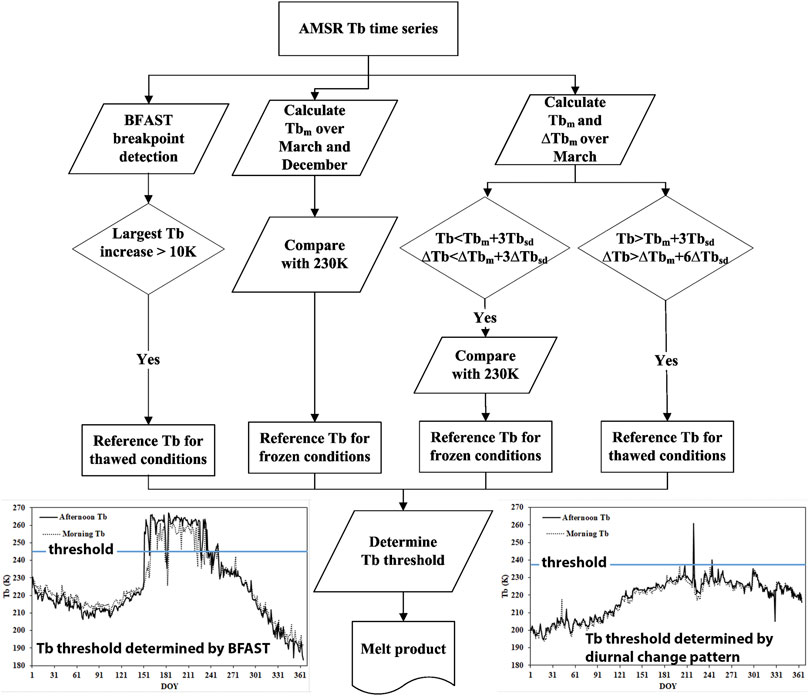
FIGURE 1. Processing flowchart for Adaptive Threshold (ADT) algorithm.

The second step in the ADT algorithm for determining a robust Tb threshold is based on the diurnal Tb variability. This approach is motivated by the fact that infrequent melt events are unlikely to generate a persistent increase in Tb sufficient to signal a BFAST algorithm break-point in the annual Tb trend. The algorithm objective is to define reference melt and frozen days based on the magnitude of diurnal Tb changes ($\Delta Tb$). Days in which the daily average $Tb>(T{b}_m+3T{b}_{sd})$ and $\Delta Tb>\left(\Delta T{b}_m+6\Delta T{b}_{sd}\right)$ (where subscripts m and sd represent the mean and standard deviation of $Tb$ or $\Delta Tb$ values over the March winter reference period) are defined as “melt,” and days in which $Tb<(T{b}_m+3T{b}_{sd})$ and $\Delta Tb<\left(\Delta T{b}_m+3\Delta T{b}_{sd}\right)$ are defined as “frozen.” The above criteria were empirically defined based on the considerations that 1) partially melted snow generally has warmer $Tb$ than dry snow under typical frozen conditions (e.g. characterized by over 99.7% or within $3T{b}_{sd}$ of the mean observed during March assuming a normal distribution of $Tb$ data); and 2) diurnal $Tb$ changes caused by melting and re-freezing events have much larger magnitude than most $\Delta Tb$ values observed during winter (e.g. larger than $6\Delta T{b}_{sd}$ beyond the mean). The average of all Tb-derived melt days is set as $T{b}_t$. $T{b}_f$ is set as the highest value between 230 K and the maximum Tb from the defined frozen days.

The BFAST approach is suitable for areas where more persistent summer melting occurs, while the diurnal Tb variability method is designed for detecting infrequent melt events or melting during the freeze/thaw transition period. For pixels where both approaches are applicable, the resulting higher Tb value is used to define the pixel-wise melt thresholds (Tb_thresh). This process is repeated annually for each pixel to update Tb melt thresholds across the GrIS in response to changing surface snow conditions (e.g. temperature, surface roughness, density, stratification, and grain size differences) that may affect baseline microwave scattering and emissions characteristics (Du et al., 2010; Du et al., 2014).

The ADT methodology was applied to 36.5V GHz Tb measurements from the NASA AMSR-E (Advanced Microwave Scanning Radiometer for EOS) sensor record, projected to a Northern Polar EASE-Grid 2.0 projection (Kim et al., 2019). Here, the AMSR-E Tb retrievals reflect different local satellite overpass times (1330 and 0130) and are projected to a finer grid resolution (6 km) closer to the native footprint of the 36.5 GHz Tb retrievals, relative to the 25 km grid resolution of the SSM/I (1730 and 0530 local time) Tb retrievals used in the other GrIS melt records for the overlapping study period (Table 1). Despite application of the same ice mask to the data, the finer 6 km grid results in a slightly different ice sheet area compared to the other products. For this reason, we presented the product comparison results as a fraction of ice area to normalize for small area changes between products.

Automatic Weather Station Data

We used on-ice weather station (AWS) temperature data from the GC-Net network as an in situ metric of melt conditions (Steffen et al., 1996). The PROMICE AWS network was also investigated for comparison, but stations in this network are generally located near the ice sheet margin where bare land conditions may influence Tb retrievals over adjacent ice cover within the same satellite footprint, and the installation dates of the majority of network stations is later than the time period of comparison in this study (seesection 2.3). Fourteen GC-Net network stations contained data for the time period of comparison, and were located far enough from the ice sheet margin to eliminate the effects of bare terrain on the collocated Tb retrievals at each AWS location. We focused our analysis on data from these AWS sites, which span the full elevation range of the GrIS. The stations used in this study are shown in Figure 2 and summarized in Table 2.

FIGURE 2

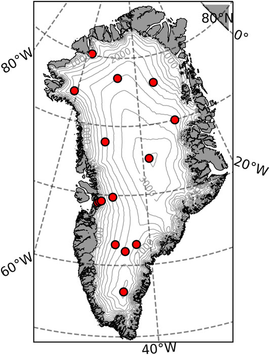
FIGURE 2. GCNet AWS site locations used in this study. Surface elevation contours in gray are displayed at 200 m intervals (Morlighem et al., 2017).

TABLE 2

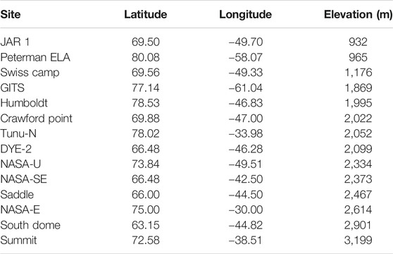
TABLE 2. AWS site locations used in the microwave product comparison.

Definition of AWS Melt Day

Comparison of satellite microwave products against the AWS observation network requires definition of a melt day threshold from the in situ measurements. Past studies have defined melt days based on a daily average temperature threshold of 0°C (e.g. Fettweis et al., 2011). Here, we used a threshold definition in closer alignment with surface mass balance modeling approaches based on temperature-index methods, which assume that melt over a given time period scales with the cumulative sum of temperatures >0°C over that time period (e.g. Hock, 2003; Hock, 2009).

An AWS melt day is defined here as one in which the daily sum of hourly air temperatures greater than 0°C exceeds 4°C h, which generates ∼1 mm of daily melt for a snow degree day factor in general agreement with published values (6 mm d⁻¹°C⁻¹ (Hock, 2003)). This melt amount is equivalent to 1% liquid water content in the upper 25 cm of a snowpack with average density of 400 kg m⁻³.

Time Period of Comparison

Threshold values used in the XPGR, DAV19 and DAV37 approaches were developed based on Tb measured on the SSM/I F11 and F13 satellite platforms, which operated from 1991 to 2008; the fidelity of these Tb thresholds on the later SSM/I F17 platform is unknown and therefore SSM/I F17 data weren’t used in this investigation. The AMSR-E Tb data, upon which the ADT method is based, are available beginning in 2002. Based upon these limiting factors, our analysis focused on the 2003–2007 period for which complete Tb annual data records were available for all products.

Results

Product Comparison Against in situ AWS Measurements

Annual Melt Day Sums and Seasonal Timing

An example of the accumulated melt days at the Swiss Camp AWS site in 2003 is presented in Figure 3. The satellite melt products match the in situ measured melt days with varying degrees of fidelity. While the melt onset date is well captured by both DAV products, cumulative melt days are substantially underpredicted. Melt onset in the ADT and TDM closely agree, and the cumulative melt days are within 5% of the AWS measurements, although ADT indicates continued melted conditions after the melt season when temperatures remain cold. Cumulative melt days determined by the XPGR and MTE also agree well with the AWS measurements, but melt onset is delayed in the XPGR and premature in the MTE, and melting persists beyond the AWS-determined melt season in both products.

FIGURE 3

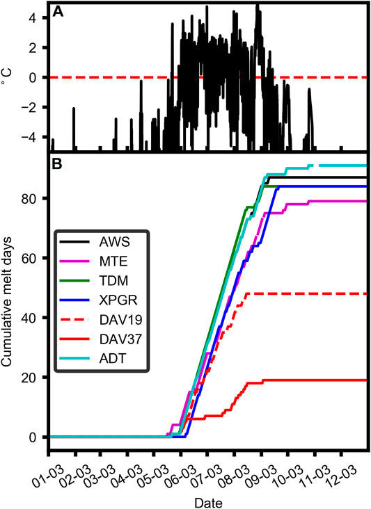
FIGURE 3. Hourly average near surface air temperature (A), and cumulative melt days from measurement and microwave products (B) at the Swiss Camp AWS in 2003. Red dashed line in (A) references 0°C temperature threshold.

Site results, like those presented in Figure 3, were summarized for all sites and years by comparing AWS and satellite derived annual melt days (Figure 4), timing of melt onset (Supplementary Figure S1), and melt termination (Supplementary Figure S2). At sites and years with >30 days of melt, both DAV products showed a low melt bias (Figure 4). This bias diminishes for low melt sites/years. In contrast, the ADT, TDM, MTE, and XPGR products agree reasonably well with observations where melt is frequent, but have a tendency to overpredict melt frequency at sites where melting is uncommon. The dates of melt termination from these four products (ADT, TDM, MTE, XPGR) showed generally better agreement with the observations (Supplementary Figure S2), compared to the date of melt onset (Supplementary Figure S1).

FIGURE 4

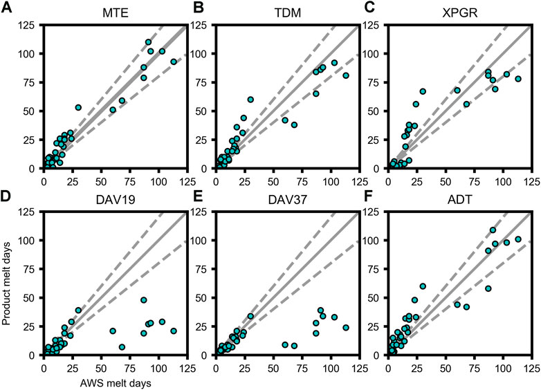
FIGURE 4. Annual melt days from AWS measurements (x-axis) and all six satellite microwave melt products (y-axis) for all sites and all years. Gray line indicates the 1:1 relationship, and dashed lines bound the ± 20% envelope for reference.

Day-To-Day Melt Day Agreement

Using annual melt days as a metric of comparison facilitates broad assessment of the agreement between AWS observations and the different satellite products on annual time scales, but does not resolve the fidelity of products at daily resolution. We therefore evaluated product agreement with AWS observations for each melt day. The results are summarized in Table 3.

TABLE 3

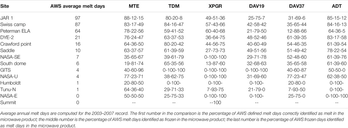
TABLE 3. Daily melt agreement between AWS measurements and satellite microwave products.

The DAV19 product failed to match more than 50% of AWS melt days at any site. The DAV37 product showed better AWS agreement than DAV19 and matched the observed melt days with the same fidelity as the other products at sites experiencing fewer than ∼20 melt days per year. The XPGR daily melt agreement was the poorest of all tested products. A large percentage of XPGR melt days occurred when the AWS measurements indicated frozen conditions, explaining the lack of a negative annual melt bias (Figure 4) despite the poor daily agreement.

Both products based on emissions modeling, MTE and TDM, showed comparable agreement with the AWS observations. At most sites, both products reproduced the AWS observed melt days with >60% agreement; although, ∼50% of the product melt days occurred when the AWS observations indicated contrasting frozen conditions. The ADT product showed overall agreement with the AWS observations that was similar to the MTE and TDM performance; thus, the ADT method appears capable of identifying melt days at a level that is commensurate with the more standard GrIS melt products. For sites with more than 1-day average annual melt period, the ADT record showed strongest agreement (68.9% AWS melt days classified as melt by ADT); and lowest disagreement (31.1% AWS melt days classified as frozen by ADT; 38.2% ADT melt days indicated as frozen by AWS) with station measurements among all of the products examined (Table 3).

Product-To-Product Comparison

An inherent limitation in evaluating ice sheet-wide melt products is the very low density of the regional AWS measurement network available for validation, which is too sparse to resolve the full range of GrIS environmental gradients. The satellite melt products were therefore compared against each other over the full GrIS domain as an additional assessment of relative model performance, in context with the more detailed AWS comparison.

The 2003–2007 average annual melt days from each microwave product are presented in Figure 5. All of the products showed similar broad spatial patterns consistent with the GrIS climatology (e.g. Reeh, 1991), including the largest number of melt days at low elevations, little or no melt in the high elevation ice sheet interior, and expanded melt conditions in western Greenland. Yet, the low melt bias indicated from the comparison of both DAV products to the AWS observations was also evident between the DAV and other products over the larger GrIS domain.

FIGURE 5

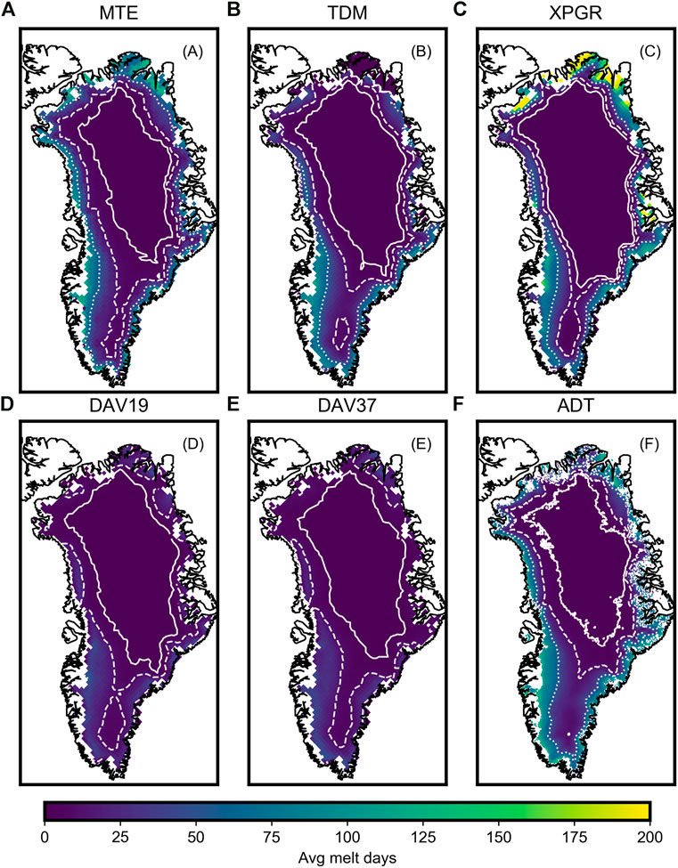
FIGURE 5. 2003-2007 average melt days over the GrIS from six microwave melt products including MTE(A), TDM(B), XPGR(C), DAV19(D), DAV37(E), and ADT(F). Solid white line is the 1-melt day contour, dashed line is the 10-day contour, and dotted line is the 50-day contour.

Product-specific spatial patterns in melting are revealed by partitioning the GrIS into melt day bins (Figure 5). The MTE indicates that nearly 45% of the GrIS experiences at least one melt day each year, while almost 15% of the GrIS experiences 50 melt days or more. Both DAV-based products indicate a significant cold bias compared to all other products; whereby, the DAV maximum cumulative melt values failed to reach 50 days for any pixel, and annual melting of 25 days or more occurred over just 4% of the GrIS. In contrast, the TDM, MTE, XPGR, and ADT results showed the same melt frequency occurring over a much larger (19–25%) portion of the GrIS. Among these four products, the ADT and MTE indicated nearly identical ice sheet fractions across the range of melt days. The XPGR showed a similar pattern, except for the highest melt intensities. The XPGR was the only product indicating >125 melt days over a portion of the ice sheet; this relatively extreme melt anomaly was also concentrated in the northernmost GrIS (Figure 6, see Discussion).

FIGURE 6

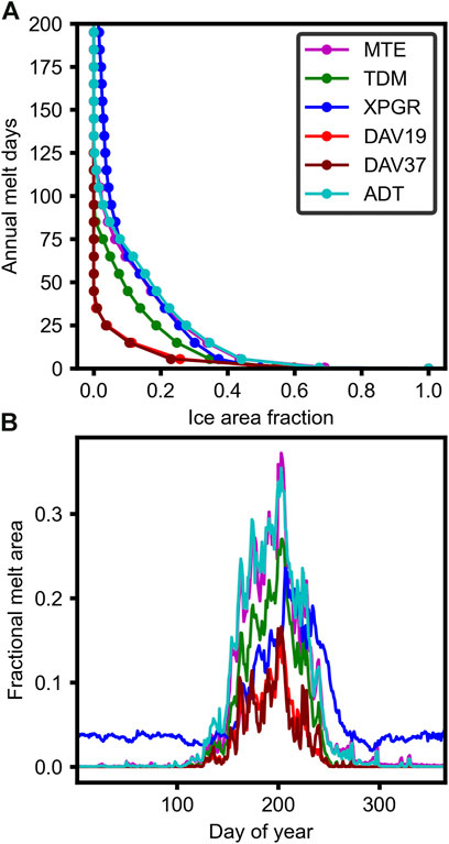
FIGURE 6. Fractional area of the GrIS versus 2003–2007 average annual melt days for each of the six tested melt products (A), and average fractional daily melt area versus time (B).

The annual melt timing, aggregated over the ice sheet, shows similarities to the in situ AWS comparison (Figure 6). On average, the DAV results showed the latest seasonal melt onset and earliest melt termination of all satellite products examined, although the TDM showed a similar melt season duration. The ADT and MTE products showed a high degree of consistency in the annual melt pattern. The XPGR results indicated a small fraction of the GrIS persistently melting through the winter period, which may reflect Tb retrieval or classification error. Both the classified melt season onset and termination in the XPGR were delayed compared to the other datasets. With the exception of the XPGR, all of the other melt products exhibited similar temporal trends in fractional melt area through the melt season. Pearson correlation coefficients between the XPGR and other melt products never exceeded 0.5, while correlation coefficients between all other melt products were >0.85 for each combination. However, despite the similarity in temporal trends, the magnitude of GrIS melt patterns and seasonal changes differed markedly among the products examined.

Discussion

Choice of Observational Melt Day Threshold

None of the products examined fully captured the melt day patterns indicated from the AWS observations. Reasons for the lack of agreement include uncertainty regarding the selected in situ melt day threshold. The threshold applied in this study is physically based, but other thresholds could no doubt be similarly justified. Daily average air temperatures exceeding 0°C have previously been used to define melt thresholds (e.g. Fettweis et al., 2011). Considering that the higher frequency Tb retreivals predominantly represent conditions within a relatively thin snow surface layer with low heat capacity, a maximum air temperature exceeding 0°C could also be justified. The choice of observational threshold can have a significant impact on the resulting microwave product agreement. For example, a melt threshold based on the maximum daily air temperature reduces the tendency of the MTE, TDM, and ADT products to overestimate melt at sites with low melt occurrence (Supplementary Figure S3). While selective tuning of microwave Tb thresholds has been commonly used to improve the agreement between remotely sensed retrievals and observations, it is important to consider the observational threshold itself, since the determination of a melting snow surface, especially from near surface air temperature measurements, is not straightforward. Associated uncertainty in assigning melt thresholds can also contribute to significant bias in the resulting satellite melt records.

Attribution of Persistent Biases

Despite the sensitivity of certain aspects of the tested melt products to the observational threshold, other persistent biases in some of the melt products were insensitive to the choice of observational melt threshold.

XPGR

The delayed melt onset and termination, and melt persistence during winter are features of the XPGR product that deviate from other products and available observations. Winter melting is concentrated around the northern and eastern GrIS margin. Comparison of the ice sheet mask against an independent mask of the Greenland land ice body from aerophotogrammetry (Citterio and Ahlstrøm, 2013) shows that a substantial fraction of the pixels with high melt (and therefore substantial winter melt days) are actually concentrated either off the ice sheet, or over peripheral glaciers where exposed bedrock likely composes a large part of the pixel (Supplementary Figure S4). The majority of the winter melt days reflect either compromised pixels or pixels that are off the ice sheet entirely. In comparison, this northern off-ice sector is masked in the TDM product. The ADT method indicates high melt conditions, but is also computed from a Tb dataset with finer resolution gridding. The identification of frequent melt events in these peripheral regions indicates that assessment of changes in conditions must carefully consider the ice mask used and the resolution of the gridded Tb product.

Supplementary Figure S4 does show some remaining anomalous ice-covered pixels indicating excessive (>200) melt days. These pixels are predominantly located in the northern GrIS near the Nares Strait, and the Northeast ice stream; both locations where regional climate modeling has shown low precipitation and high melt rates (Ettema et al., 2009). It is plausible that bare ice is exposed for a substantial fraction of the year at these locations. Bare ice emission is acknowledged to be microwave frequency independent, and the tendency to classify frozen bare ice as melt is a known limitation of the algorithm (Abdalati and Steffen, 1997). This is a plausible cause of the anomalous winter melt pixels. Moreover, it is also possible that this effect persists over larger swaths of the GrIS ablation zone at the end of the melt season when conditions are frozen, but measurable snowfall has yet to occur. Thus, bare ice effects may also contribute to the delayed end of the XPGR melt season (Figure 6).

The causal mechanism for the delayed melt onset in the XPGR is less clear. Fettweis et al. (2005); Fettweis et al. (2006) identified a shortcoming of the XPGR algorithm to determine melt conditions during rainfall events when greater abundance of precipitable water vapour in the atmospheric column obscured the surface Tb signal. However, it is unlikely that this factor would cause the consistently observed delay in XPGR melt onset (Supplementary Figure S1), as this would require significant rainfall at the start of the melt season across all AWS sites.

A more likely cause of the delayed XPGR melt season is uncertainty regarding the algorithm melt threshold selection, which Abdalati and Steffen (1997) acknowledged to be heuristic. A different threshold could be defined based on a lower measured liquid water content as in Abdalati and Steffen (1995), which may improve XPGR timing with respect to both AWS measurements and other satellite melt products. However, the 1% measured liquid water content upon which the threshold used in this study is based, was motivated in part to maintain consistency with the model framework of Mote and Anderson (1995). The differences in melt timing between the MTE and XPGR products (Figure 6) illustrates the sensitivity of melt determination to the underlying methodology, even when melt thresholds are based on the same snowpack conceptual framework.

DAV

The DAV method was originally developed for quantifying the onset and termination of melt in coastal Alaska and British Columbia (Ramage and Isacks, 2002; Ramage and Isacks, 2003). In these more temperate climates with mild temperatures and frequent melt, persistent liquid water in the snowpack was clearly detectable during the summer melt season using a daily average Tb threshold. But this threshold failed to identify melt during the shoulder seasons, when liquid water content was relatively low and tended to refreeze overnight. Quantifying the diurnal variability in Tb between satellite AM and PM overpasses was therefore developed as a sensitive method to elucidate these less intensive ephemeral melt events.

With this in mind, it is surprising that the DAV generally produced less melt than the other satellite melt products. However, in applying the DAV method over the GrIS, the additional constraint that the daily average Tb must exceed a defined threshold is also imposed. This additional constraint is congruent with the more conservative “melt method” used by Ramage and Isaacks, (2002), Ramage and Isaacks, (2003), and reduces the sensitivity of melt determination contributed from the Tb diurnal range, which the method was originally intended to identify. Moreover, the daily average Tb and diurnal range thresholds for both 19 and 37 GHz channels are also invariant over the GrIS. This neglects the inherent variability in snow surface characteristics that may lead to differing baseline Tb levels upon which diurnal variations from daily melting and refreezing are superimposed. This is perhaps most apparent in the distinction between bare ice cover in the ablation zone, and the more permanent snow cover deeper in the ice sheet interior. Introduction of spatially varying thresholds would likely improve the DAV product, particularly at locations with higher melt frequency, where the product has a tendency to underestimate melt.

ADT Performance

The new ADT method for melt determination presented in this study performs at a similar level as the emission model based approaches, despite the different ADT methodology that incorporates information from both the Tb seasonal trend and diurnal amplitude, and is more heuristic in implementation. The relatively consistent performance of the three different methodologies is encouraging, and implies that, at broad scale, the observed brightness temperature changes reflect a change in emission characteristics that is robust. In particular, for sites with more than 1-day average annual melt period, the ADT showed the best performance (section 3.1.2) among all of the products examined. The ADT also only uses satellite Tb observations as model inputs and doesn’t require any additional ancillary data. The higher ADT performance likely benefits from the finer spatial gridding of the AMSR-E Tb inputs, which improves the delineation of GrIS melt events, especially over heterogeneous areas with mixed melt and frozen conditions.

Implications for GrIS Melt Monitoring

As Greenland melting increases, understanding the extent, intensity, and fate of meltwater is of increasing importance. As much as nearly 60% of meltwater may be retained on the ice sheet (van den Broeke et al., 2016) in firn pore space. Future sea level contributions from the ice sheet depend in part on how melt sequestration evolves in the ice sheet interior (Harper et al., 2012), motivating the need to understand the state and evolution of areas of the GrIS with low melt frequency.

Despite their relatively large variation in estimated melt rates, the high temporal fidelity, long-term observational records and global coverage of the satellite passive microwave melt products make them an important source for monitoring changes in the GrIS interior. At AWS sites experiencing fewer than ∼20 melt days per year, the measurement - product agreement is good for the ADT method. Similar good agreement with the AWS observations was also found for the emissions-model based TDM and MTE, and DAV37 products (Table 3). Yet, at this low melt frequency, the results indicate that large spatial variability still persists among the four products (Figure 5), implying a wide variation in Tb-determined percolation zone extent. For example, the Crawford Point AWS site averaged 16 melt days over the same period (Table 3), where core site measurements indicated ∼27% (by mass) of the annual snow accumulation melted and refroze during 2003–2006 (Higgins, 2012). Thus, despite the relatively low number of melt days, this region of the ice sheet where melt products show wide variation experiences significant melt and refreezing volumes.

The relatively large variation in estimated melt area indicated from the different satellite products indicates that delineation of melting from passive microwave measurements is quite sensitive to the underlying algorithm and product choice. Nevertheless, all products do agree in the sense that the GrIS melt area rate of change has been increasing since the early 1990s (Mote, 2007; Tedesco, 2007), a result that is also consistent with regional climate model projections (Fettweis et al., 2011). Thus, while the trend in melt area at the ice sheet scale is likely robust, the melt frequency at any particular location is more uncertain, which may contribute to uncertainty in site or region-specific details of melt frequency and history. Further analysis combining process model simulations and the remote sensing products with clearly-defined uncertainties is expected to improve the quantification of Greenland snow/ice melting and its impact on the rate and trend of ice sheet loss.

Conclusion

We evaluated six different satellite passive microwave-based melt products over a common 5-year study period for their ability to capture the timing and pattern of daily melt events in relation to each other and against independent weather station (AWS) observations from 14 sites located across the GrIS. The satellite products are derived from similar satellite sensors and Tb frequencies (19–37 GHz), but using different retrieval algorithms to determine daily melt conditions. The different retrieval algorithms included physics-based modeling of Tb melt thresholds, diurnal Tb variability, and changes in the ratio of cross-polarized 19 and 37 GHz Tb channels. The satellite products examined in this study also included a new adaptive threshold (ADT) method for daily melt classification that employs a two-step process to identify melt thresholds based on temporal breaks in the seasonal Tb trend and the Tb diurnal amplitude.

Comparison of the different melt products showed variable agreement with AWS observations and between the different products, where the relative differences in product performance were largely attributed to differences in the underlying classification algorithms and model assumptions. The two emission model-based approaches (MTE, TDM) and the newly developed ADT method generally agreed most closely with the AWS measurements. In particular, for sites experiencing moderate to high melt occurrence (>1 day per year), the ADT results showed the best performance among all of the products examined (68.9% of AWS melt days classified as melt by the ADT; 31.1% of AWS melt days classified as frozen by the ADT; and 38.2% of ADT melt days classified as frozen by AWS measurements) (Table 3). However, the satellite products showed a larger spread and less agreement with the AWS observations over the GrIS interior where melt events occur more infrequently further from the ice margin. In this interior region of the GrIS, only the ADT succeeded in matching AWS measurement-based melt days at a level exceeding 50%.

While the theoretical influence of liquid water on snowpack emission properties is clear (Ulaby et al., 1986), our results show that, in practice, correctly identifying a snowmelt event from satellite microwave Tb observations remains sensitive to decisions made in how best to capture the changing wetness within a relatively coarse sensor footprint. Satellite monitoring of melt dynamics over the GrIS has strong utility for verifying regional climate models and as a sensitive climate indicator of changing ice sheet conditions. However, while the different products and underlying classification methods analysed in this study were broadly consistent in documenting ice sheet-wide conditions, the products showed significant spread in classifying melt events for different locations, particularly where melting occurs infrequently. Our results identify the characterization of effective Tb surface melt thresholds as a key constraint and potential focus area for further algorithm and product enhancements. Further enhancements may be gained by exploiting the varying sensitivities and sampling footprints from multiple microwave frequencies which offer the potential for both spectral and spatial enhancement of surface melt.

Data Availability Statement

The original contributions presented in the study are included in the article/Supplementary Material, further inquiries can be directed to the corresponding author/s.

Author Contributions

JD, JK, and TM conceived the study. JD developed the new method for melt determination. TM performed analysis of published products. All authors contributed project guidance and manuscript writing.

Funding

This work was conducted at the University of Montana with funding provided by NASA (80NSSC18K0980) and Montana NASA EPSCoR (G185-19-W5586).

Conflict of Interest

The authors declare that the research was conducted in the absence of any commercial or financial relationships that could be construed as a potential conflict of interest.

Publisher’s Note

All claims expressed in this article are solely those of the authors and do not necessarily represent those of their affiliated organizations, or those of the publisher, the editors and the reviewers. Any product that may be evaluated in this article, or claim that may be made by its manufacturer, is not guaranteed or endorsed by the publisher.

Supplementary Material

The Supplementary Material for this article can be found online at: https://www.frontiersin.org/articles/10.3389/feart.2021.654220/full#supplementary-material

References

Abdalati, W., and Steffen, K. (1995). Passive Microwave-Derived Snow Melt Regions on the Greenland Ice Sheet. Geophys. Res. Lett. 22, 787–790. doi:10.1029/95GL00433

CrossRef Full Text | Google Scholar

Abdalati, W., and Steffen, K. (1997). Snowmelt on the Greenland Ice Sheet as Derived from Passive Microwave Satellite Data. J. Clim. 10, 165–175. doi:10.1175/1520-0442(1997)010<0165:sotgis>2.0.co;2

CrossRef Full Text | Google Scholar

Chen, X., Zhang, X., Church, J. A., Watson, C. S., King, M. A., Monselesan, D., et al. (2017). The Increasing Rate of Global Mean Sea-Level Rise During 1993-2014. Nat. Clim Change. 7, 492–495. doi:10.1038/nclimate3325

CrossRef Full Text | Google Scholar

Citterio, M., and Ahlstrøm, A. P. (2013). Brief Communication "The Aerophotogrammetric Map of Greenland Ice Masses". The Cryosphere. 7, 445–449. doi:10.5194/tc-7-445-2013

CrossRef Full Text | Google Scholar

Du, J., Kimball, J. S., Azarderakhsh, M., Dunbar, R. S., Moghaddam, M., and McDonald, K. C. (2014). Classification of Alaska Spring Thaw Characteristics Using Satellite L-Band Radar Remote Sensing. IEEE Trans. Geosci. Remote Sens. 53, 542–556. doi:10.1109/tgrs.2014.2325409

CrossRef Full Text | Google Scholar

Du, J., Shi, J., and Rott, H. (2010). Comparison Between a Multi-Scattering and Multi-Layer Snow Scattering Model and its Parameterized Snow Backscattering Model. Remote. Sens. Environ. 114, 1089–1098. doi:10.1016/j.rse.2009.12.020

CrossRef Full Text | Google Scholar

Enderlin, E. M., Howat, I. M., Jeong, S., Noh, M.-J., Van Angelen, J. H., and Van Den Broeke, M. R. (2014). An Improved Mass Budget for the Greenland Ice Sheet. Geophys. Res. Lett. 41, 866–872. doi:10.1002/2013GL059010

CrossRef Full Text | Google Scholar

Ettema, J., van den Broeke, M. R., van Meijgaard, E., van de Berg, W. J., Bamber, J. L., Box, J. E., et al. (2009). Higher Surface Mass Balance of the Greenland Ice Sheet Revealed by High-Resolution Climate Modeling. Geophys. Res. Lett. 36, L12501. doi:10.1029/2009GL038110

CrossRef Full Text | Google Scholar

Fettweis, X., Box, J. E., Agosta, C., Amory, C., Kittel, C., Lang, C., et al. (2017). Reconstructions of the 1900-2015 Greenland Ice Sheet Surface Mass Balance Using the Regional Climate MAR Model. The Cryosphere. 11, 1015–1033. doi:10.5194/tc-11-1015-2017

CrossRef Full Text | Google Scholar

Fettweis, X., Gallée, H., Lefebre, F., and van Ypersele, J.-P. (2005). Greenland Surface Mass Balance Simulated by a Regional Climate Model and Comparison with Satellite-Derived Data in 1990-1991. Clim. Dyn. 24, 623–640. doi:10.1007/s00382-005-0010-y

CrossRef Full Text | Google Scholar

Fettweis, X., Gallée, H., Lefebre, F., and van Ypersele, J.-P. (2006). The 1988-2003 Greenland Ice Sheet Melt Extent Using Passive Microwave Satellite Data and a Regional Climate Model. Clim. Dyn. 27, 531–541. doi:10.1007/s00382-006-0150-8

CrossRef Full Text | Google Scholar

Fettweis, X., Tedesco, M., van den Broeke, M., and Ettema, J. (2011). Melting Trends over the Greenland Ice Sheet (1958-2009) from Spaceborne Microwave Data and Regional Climate Models. The Cryosphere. 5, 359–375. doi:10.5194/tc-5-359-2011

CrossRef Full Text | Google Scholar

Fettweis, X., van Ypersele, J.-P., Gallée, H., Lefebre, F., and Lefebvre, W. (2007). The 1979-2005 Greenland Ice Sheet Melt Extent from Passive Microwave Data Using an Improved Version of the Melt Retrieval XPGR Algorithm. Geophys. Res. Lett. 34, 1–5. doi:10.1029/2006GL028787

CrossRef Full Text | Google Scholar

Foster, J. L., Hall, D. K., Chang, A. T. C., and Rango, A. (1984). An Overview of Passive Microwave Snow Research and Results. Rev. Geophys. 22, 195–208. doi:10.1029/rg022i002p00195

CrossRef Full Text | Google Scholar

Friedl, M. A., McIver, D. K., Hodges, J. C. F., Zhang, X. Y., Muchoney, D., Strahler, A. H., et al. (2002). Global Land Cover Mapping from MODIS: Algorithms and Early Results. Remote. Sens. Environ. 83, 287–302. doi:10.1016/S0034-4257(02)00078-0

CrossRef Full Text | Google Scholar

Harper, J., Humphrey, N., Pfeffer, W. T., Brown, J., and Fettweis, X. (2012). Greenland Ice-Sheet Contribution to Sea-Level Rise Buffered by Meltwater Storage in Firn. Nature 491, 240–243. doi:10.1038/nature11566

PubMed Abstract | CrossRef Full Text | Google Scholar

Higgins, L. (2012). Construction and Analysis of an Ice Core-Derived Melt History from West Central Greenland (1765-2006). Available at: https://etd.ohiolink.edu/pg_10?::NO:10:P10_ETD_SUBID:76225 (Accessed October 1, 2020).

Google Scholar

Hock, R. (2005). Glacier Melt: A Review of Processes and Their Modelling. Prog. Phys. Geogr. Earth Environ. 29, 362–391. doi:10.1191/0309133305pp453ra

CrossRef Full Text | Google Scholar

Hock, R. (2003). Temperature index Melt Modelling in Mountain Areas. J. Hydrol. 282, 104–115. doi:10.1016/S0022-1694(03)00257-9

CrossRef Full Text | Google Scholar

Kim, Y., Kimball, J. S., Glassy, J., and Du, J. (2017). An Extended Global Earth System Data Record on Daily Landscape Freeze-Thaw Status Determined from Satellite Passive Microwave Remote Sensing. Earth Syst. Sci. Data. 9, 133–147. doi:10.5194/essd-9-133-2017

CrossRef Full Text | Google Scholar

Kim, Y., Kimball, J. S., Glassy, J., and McDonald, K. C. (2019). MEaSUREs Northern Hemisphere Polar EASE-Grid 2.0 Daily 6 Km Land Freeze/Thaw Status from AMSR-E and AMSR2, Version 1. Boulder, CO: NASA National Snow and Ice Data Center Distributed Active Archive Center. doi:10.5067/WM9R9LQ2SA85

CrossRef Full Text | Google Scholar

Liu, H., Wang, L., and Jezek, K. C. (2005). Wavelet‐transform Based Edge Detection Approach to Derivation of Snowmelt Onset, End and Duration from Satellite Passive Microwave Measurements. Int. J. Remote Sensing. 26 (21), 4639–4660. doi:10.1080/01431160500213342

CrossRef Full Text | Google Scholar

Morlighem, M., Williams, C. N., Rignot, E., An, L., Arndt, J. E., Bamber, J. L., et al. (2017). BedMachine V3: Complete Bed Topography and Ocean Bathymetry Mapping of Greenland from Multibeam Echo Sounding Combined with Mass Conservation. Geophys. Res. Lett. 44, 11051–11061. doi:10.1002/2017GL074954.Mote

PubMed Abstract | CrossRef Full Text | Google Scholar

Mote, T. L., and Anderson, M. R. (1995). Variations in Snowpack Melt on the Greenland Ice Sheet Based on Passive-Microwave Measurements. J. Glaciol. 41, 51–60. doi:10.1017/S0022143000017755

CrossRef Full Text | Google Scholar

Mote, T. L. (2007). Greenland Surface Melt Trends 1973–2007: Evidence of a Large Increase in 2007. Geophys. Res. Lett. 34, L22507. doi:10.1029/2007GL031976

CrossRef Full Text | Google Scholar

Nghiem, S. V. (2005). Mapping of Ice Layer Extent and Snow Accumulation in the Percolation Zone of the Greenland Ice Sheet. J. Geophys. Res. 110, F02017. doi:10.1029/2004JF000234

CrossRef Full Text | Google Scholar

Pulliainen, J. T., Grandell, J., and Hallikainen, M. T. (1999). HUT Snow Emission Model and its Applicability to Snow Water Equivalent Retrieval. IEEE Trans. Geosci. Remote Sensing. 37 (3), 1378–1390. doi:10.1109/36.763302

CrossRef Full Text | Google Scholar

Ramage, J. M., and Isacks, B. L. (2002). Determination of Melt-Onset and Refreeze Timing on Southeast Alaskan Icefields Using SSM/I Diurnal Amplitude Variations. Ann. Glaciol. 34, 391–398. doi:10.3189/172756402781817761

CrossRef Full Text | Google Scholar

Ramage, J. M., and Isacks, B. L. (2003). Interannual Variations of Snowmelt and Refreeze Timing on Southeast-Alaskan Icefields, U.S.A. J. Glaciol. 49, 102–116. doi:10.3189/172756503781830908

CrossRef Full Text | Google Scholar

Reeh, N. (1991). Parameterization of Melt Rate and Surface Temperature in the Greenland Ice Sheet. Polarforschung 5913, 113–128. Available at: hdl:10013/epic.29636.d001

Google Scholar

Steffen, K., Box, J. E., and Abdalati, W. (1996). “Greenland Climate Network: GC-Net,” in CRREL 96-27 Special Report on Glaciers, Ice Sheets and Volcanoes, Trib. To M. Meier. Editor S. C. Colbeck, Hanover: New Hampshire. 98–103.

Google Scholar

Steiner, N., and Tedesco, M. (2014). A Wavelet Melt Detection Algorithm Applied to Enhanced-Resolution Scatterometer Data over Antarctica (2000-2009). The Cryosphere. 8 (1), 25–40. doi:10.5194/tc-8-25-2014

CrossRef Full Text | Google Scholar

Tedesco, M. (2009). Assessment and Development of Snowmelt Retrieval Algorithms over Antarctica from K-Band Spaceborne Brightness Temperature (1979-2008). Remote. Sens. Environ. 113, 979–997. doi:10.1016/j.rse.2009.01.009

CrossRef Full Text | Google Scholar

Tedesco, M., Fettweis, X., Mote, T., Wahr, J., Alexander, P., Box, J. E., et al. (2013). Evidence and Analysis of 2012 Greenland Records from Spaceborne Observations, a Regional Climate Model and Reanalysis Data. The Cryosphere. 7, 615–630. doi:10.5194/tc-7-615-2013

CrossRef Full Text | Google Scholar

Tedesco, M., and Fettweis, X. (2020). Unprecedented Atmospheric Conditions (1948-2019) Drive the 2019 Exceptional Melting Season over the Greenland Ice Sheet. The Cryosphere. 14, 1209–1223. doi:10.5194/tc-14-1209-2020

CrossRef Full Text | Google Scholar

Tedesco, M., Fettweis, X., van den Broeke, M. R., van de Wal, R. S. W., Smeets, C. J. P. P., van de Berg, W. J., et al. (2011). The Role of Albedo and Accumulation in the 2010 Melting Record in Greenland. Environ. Res. Lett. 6, 014005. doi:10.1088/1748-9326/6/1/014005

CrossRef Full Text | Google Scholar

Tedesco, M. (2014). Greenland Daily Surface Melt 25km EASE-Grid EASE-Grid, (2001-2015), New York, NY: City College of New York, The City University of New York. Digital media. 2003–2007.

Tedesco, M. (2007). Snowmelt Detection over the Greenland Ice Sheet from SSM/I Brightness Temperature Daily Variations. Geophys. Res. Lett. 34, 1–6. doi:10.1029/2006GL028466

CrossRef Full Text | Google Scholar

Ulaby, F. T., Moore, R. K., and Fung, A. K. (1986). Microwave Remote Sensing: Active and Passive, Volume III: From Theory to Application. Editor D. S. Dimonett Dedham (Norwood, MA: Artech House, Inc).

van den Broeke, M. R., Enderlin, E. M., Howat, I. M., Kuipers Munneke, P., Noël, B. P. Y., van de Berg, W. J., et al. (2016). On the Recent Contribution of the Greenland Ice Sheet to Sea Level Change. The Cryosphere. 10, 1933–1946. doi:10.5194/tc-10-1933-2016

CrossRef Full Text | Google Scholar

Verbesselt, J., Hyndman, R., Newnham, G., and Culvenor, D. (2010). Detecting Trend and Seasonal Changes in Satellite Image Time Series. Remote. Sens. Environ. 114, 106–115. doi:10.1016/j.rse.2009.08.014

CrossRef Full Text | Google Scholar

Verbesselt, J., Zeileis, A., and Herold, M. (2012). Near Real-Time Disturbance Detection Using Satellite Image Time Series. Remote. Sens. Environ. 123, 98–108. doi:10.1016/j.rse.2012.02.022

CrossRef Full Text | Google Scholar