Combining Argo and Satellite Data Using Model-Derived Covariances: Blue Maps

1 Introduction

There are many gridded products that use Argo and other data to produce global estimates of temperature and salinity at different depths¹. These products can be grouped under two broad categories: observation-based and model-based. Most observation-based products are coarse-resolution (e.g., Ridgway et al., 2002; Roemmich and Gilson, 2009; Guinehut et al., 2012; Locarnini et al., 2013; Schmidtko et al., 2013; Zweng et al., 2013, with horizontal grid spacing of 0.5–1°). Model-based products, here restricted to ocean reanalyses that assimilate observations into an ocean general circulation model, include systems with coarse-resolution (e.g., Kohl and Stammer, 2007; Yin et al., 2011; Balmaseda et al., 2012; Köhl, 2015), some that are eddy-permitting (e.g., Carton and Giese, 2006; Carton and Giese, 2008; Ferry et al., 2007), and others that can be regarded as eddy-resolving (e.g., Oke et al., 2005; Oke et al., 2013c; Artana et al., 2019).

An important difference between all of the observation-based products is their assumptions about the background error covariance. All systems use some variant of objective analysis, and they all represent the influence of topography and land on the background error covariance in different ways. Some observation-based products are climatologies, including a mean state and seasonal cycle (e.g., Ridgway et al., 2002; Locarnini et al., 2013; Zweng et al., 2013), and others include monthly (or weekly) fields and span many years (e.g., Roemmich and Gilson, 2009; Guinehut et al., 2012; Good et al., 2013; Schmidtko et al., 2013; Ishii et al., 2017). Most observation-based products perform calculations on pressure surfaces (e.g., Roemmich and Gilson, 2009), but a few operate on isopycnal surfaces (e.g., Schmidtko et al., 2013). Most observation-based products use only Argo data (e.g., Roemmich and Gilson, 2009), or Argo data plus other in situ data (e.g., Ridgway et al., 2002). Systems that use both in situ and satellite data are less common—Guinehut et al. (2012) is a notable exception. A compelling feature of observation-based products is that they usually “fit” observations quite well. But a possible limitation of this group of products is that most are coarse-resolution, and most don’t exploit all of the available observations (most don’t use satellite data; though again Guinehut et al. (2012), is an exception).

Like observation-based products, perhaps the most important difference between the model-based products is also how each system estimates the background error covariance. Some systems use objective analysis (e.g., Carton and Giese, 2008), some use variational data assimilation (e.g., Kohl and Stammer, 2007; Köhl, 2015), and some use ensemble data assimilation (e.g., Oke et al., 2013c; Artana et al., 2019). A compelling feature of model-based products is that virtually all systems combine Argo data with other in situ data and satellite data, and all produce gridded estimates of all variables—even variables that are not systematically observed, such as velocity. Moreover, model-based products yield estimates that are somewhat dynamically-consistent, including the influence of topography, land, surface forcing, and ocean dynamics. Most systems are not precisely dynamically-consistent, since most do not conserve properties during the assimilation step, when the model fields are adjusted to better match observations. However, on the down-side, model-based products often “fit” observations relatively poorly (Oke et al., 2012; Balmaseda et al., 2015; Ryan et al., 2015; Shi et al., 2017), and many systems are hampered by model-bias (e.g., Oke et al., 2013c).

Blue Maps version 1.0, presented here, is intended to exploit the strengths of both groups of systems, delivering a product with the accuracy of an observation-based product, with the comprehensive ocean representation of a model-based system. We show here that Blue Maps produces gridded estimates with greater accuracy than model-based products, and with more versatility than observation-based products.

This paper is organised with details of the analysis system presented in Section 2, results in Section 3, an analysis and discussion in Section 4, and conclusions in Section 5.

2 Analysis System

The name, Blue Maps, is intended to acknowledge the origin of the data assimilation system used here—developed under the Bluelink Partnership (Schiller et al., 2020); acknowledge the statistical category for the method—a Best Linear Unbiased Estimate (BLUE); and acknowledge that the tool is intended for deep-water applications (Blue water). The method used to produce analyses for Blue Maps is Ensemble Optimal Interpolation (EnOI; Oke, 2002; Evensen, 2003), and the code-base is EnKF-C (Sakov, 2014), implemented with the EnOI option. Variants of EnOI are widely used to perform ocean reanalyses and forecasts on global scales (e.g., Oke et al., 2005; Brassington et al., 2007; Oke et al., 2013c; Lellouche et al., 2013; Lellouche et al., 2018; Artana et al., 2019) and regional scales (e.g., Counillon and Bertino, 2009; Xie and Zhu, 2010; Oke et al., 2013a; Sakov and Sandery, 2015). Arguably the most important elements of any configuration of EnOI, or an Ensemble Kalman Filter (the “optimal,” but more expensive, “parent” of EnOI) are the ensemble construction, the ensemble size, and the localisation length-scales. To understand this, consider the simplified analysis equation:

${\mathbf{w}}^a={\mathbf{w}}^b+{\mathbf{w}}^{inc}(1)$

$={\mathbf{w}}^b+\stackrel{n}{{\displaystyle \sum }_{i=1}}{\mathbf{c}}_i\left(x,y\right).{\mathbf{A}}_i\left(x,y,z\right),(2)$

where $\mathbf{w}$ is the state vector (here, this is temperature, salinity, and sea-level on a 1/10° grid), $\mathbf{A}$ is the ensemble of model anomalies, $\mathbf{c}$ is the weights of the ensemble members, superscripts a, b, and $inc$ denote analysis, background, and increment fields; subscripts i denote the $ith$ ensemble member; n is the ensemble size; and x, y, and z are dimensions in space (z is the vertical dimension).

To understand the importance of the ensemble construction, recognise that the increments of the state ${\mathbf{w}}^{inc}$, are constructed by projecting the background innovations (the differences between the observations and the background field) onto the ensemble. Projections are made for each horizontal grid point, using only observations that fall within the localisation radius. These projections yield two-dimensional maps of ensemble weights $\mathbf{c}$, for each ensemble member (note that these are two-dimensional because the system uses horizontal localisation, and not vertical localisation). From Eq. 2 it is clear that the ensemble is important—determining the features that can be represented in the increment field. If some feature is absent in the ensemble—say, for example, there are no ensemble members with anomalies associated with an eddy in some particular region, increments resembling anomalies associated with an eddy cannot be sensibly constructed with a linear combination of those members for that region. The ensemble should include anomalies that reflect the adjustments needed to bring the background field into closer agreement with the assimilated observations.

To understand the importance of the localisation radius, note again that for the projections at each horizontal grid point, only observations that fall within the localisation radius are used, and that the influence of an observation on that projection is reduced with distance from that grid point. If the localisation radius is too short—perhaps shorter than the typical distance between observations—then there may be insufficient observations to reliably perform the projection for a given grid point. This can result in increments with spatial scales that are not resolved by the observing system, effectively introducing noise to the analyses. Conversely, if the localisation length-scale is too long, then there may be too few degrees of freedom (depending on ensemble size—see below) for each projection to “fit” the observations (e.g., Oke et al., 2007). For ensemble-based applications, the localisation function is effectively an upper-bound on the assumed background error covariance. The effective length-scales in the ensemble-based covariance can be shorter, but not longer, than the localisation function.

To further understand the importance of the ensemble size, considering Eq. 2. If the ensemble is too small to “fit” the background innovations, then the quality of the analyses will be poor, yielding analysis innovations (differences between the observations and analysis fields) that are large. The assimilation process is somewhat analogous to the deconstruction of a time-series into Fourier components; or the approximation of some field by projecting onto a set of basis functions, using a least-square fit. Extending the analogy of the Fourier transformation, if the full spectrum is permitted, then all the details of an unbiased time-series can be represented. But if only a few Fourier components are permitted, then the deconstruction will deliver an approximation. If the Fourier components are chosen unwisely, excluding some dominant frequencies for example, then the deconstructed signal may be a very poor approximation of the original time-series. In the same way, to allow for an accurate assimilation, the ensemble must have a sufficient number and diversity of anomaly fields to permit an accurate projection of the background innovations.

Guided by the understanding outlined above, for any application, it is preferable to use the largest possible ensemble size. This is usually limited by available computational resources (e.g., Keppenne and Rienecker, 2003). If the ensemble is too small, then a shorter localisation radius is needed, to eliminate the impacts of spurious ensemble-based covariances that will degrade the analyses (e.g., Oke et al., 2007). If the localisation radius is too large, then there may be insufficient degrees of freedom for each projection, and the analyses will not “fit” the observations with “appropriate accuracy.” By “appropriate accuracy,” we mean that analyses “fit” the observations according to their assumed errors (i.e., not a perfect fit, but a fit that is consistent with the assumed observation and background field errors—the target for any Best Linear Unbiased Estimate; e.g., Henderson, 1975). These factors require a trade-off, and some tuning.

What’s the status-quo for the ocean data assimilation community? It’s typical for EnOI- or EnKF-applications for ocean reanalyses or forecasts to use an ensemble size of 100–200 (e.g., Xie and Zhu, 2010; Fu et al., 2011; Sakov et al., 2012; Oke et al., 2013c; Sakov and Sandery, 2015). By some reports, an ensemble of greater than 100 is regarded as a large ensemble (e.g., Ngodock et al., 2006, 2020). Moreover, such applications typically use localisation length-scales of 100–300 km (e.g., Fu et al., 2011; Sakov et al., 2012; Oke et al., 2013c; Sakov and Sandery, 2015; Lellouche et al., 2018; Artana et al., 2019). Importantly, most of the quoted-localisation length-scales use a quasi-Gaussian function with compact support (Gaspari and Cohn, 1999). This function reduces to zero over the quoted length-scale; and so the e-folding scale for these applications is typically about one third of the stated length-scale. These systems all assimilate in situ data and satellite data. In situ data are dominated by Argo, with nominally 300 km between profiles, and satellite data includes along-track altimeter data, with typically 100 km between tracks. For most cases, the e-folding length-scale of the localisation length-scales—and hence the background error covariance—is shorter than the nominal resolution of these key components of the global ocean observing system. This seems to be a feature of ocean reanalysis and forecasts systems that has long been over-looked by the ocean data assimilation community.

For contrast to the typical configuration for ocean reanalyses, summarised above, consider the key elements of a widely-used observation-based product. Roemmich and Gilson (2009) describe an analysis system that maps Argo data to construct gridded temperature and salinity on a 1°-resolution grid. They perform objective analysis on different pressure levels independently, and estimate the background error covariance using a correlation function that is the sum of two Gaussian functions—one with an e-folding length-scale of 140 km, and one with an e-folding scale of 1,111 km. Furthermore, Roemmich and Gilson (2009) elongate the zonal length-scales at low latitudes. Their choice of background error correlation was reportedly guided by characteristics of altimetric measurements (Zang and Wunsch, 2001). This set-up uses much longer length-scales than most model-based products, and projects observations onto a coarser grid.

For Blue Maps, we calculate weekly analyses of temperature, salinity, and sea-level anomaly (SLA) by assimilating observations into a background field that is updated using damped persistence. The horizontal grid is 1/10°-resolution, and the vertical grid increases with depth, from 5 m spacing at the surface to 150 m at 1,500 m depth. Starting with climatology, using the 2013 version of the World Ocean Atlas (WOA13; Zweng et al., 2013; Locarnini et al., 2013), consecutive analyses are calculated:

${\mathbf{w}}_j^a={\mathbf{w}}_j^b+\mathbf{K}\left(\mathbf{y}-\mathbf{H}{\mathbf{w}}_j^b\right),(3)$

where

${\mathbf{w}}_j^b=0.8{\mathbf{w}}_{j-1}^a+0.2{\mathbf{w}}_j^c,(4)$

where $\mathbf{K}$ is the gain; $\mathbf{y}$ is a vector of observations; $\mathbf{H}$ is an operator that interpolates from state-space to observation-space; the superscript c denotes climatology (for time of year), and the subscript j denotes the time index. The gain matrix $\mathbf{K}$ depends on the assumed ensemble-based background error covariance and the assumed observation error covariance (here assumed to be diagonal, with diagonal elements given the values of assumed observation error variance). EnKF-C calculates analyses using a localisation method called local analysis (Evensen, 2003; Sakov and Bertino, 2011; Sakov, 2014), using a localisation function that is quasi-Gaussian (Gaspari and Cohn, 1999). The weighted sum of the analysis field and climatology, in Eq. 4, is equivalent to damped persistence, with an e-folding timescale of approximately 14 days.

Observations assimilated into Blue Maps include profiles of temperature and salinity, satellite Sea-Surface Temperature (SST), and along-track SLA. The only in situ data used here is Argo data (Roemmich et al., 2019), sourced from the Argo Global Data Acquisition Centres, and include only data with Quality Control flags of one and two (meaning data are good, or probably good; Wong et al., 2020). The assumed standard deviation of the observation error for Argo data is 0.05°C for temperature and 0.05 practical salinity units (psu) for salinity. The instrument error of Argo temperature data is 0.002°C and for salinity is 0.01°psu (Wong et al., 2020), so the larger errors assumed here include a modest estimate for the representation error (e.g., Oke and Sakov, 2008). SLA data are sourced from the Radar Altimeter Database System (RADS Ver. 2, Scharroo et al., 2013), and include corrections for astronomical tides and inverse barometer effects. The assumed standard deviation of the observation error for SLA is 3 cm for Jason-2 and Jason-3, 4 cm for Saral, 5 cm for Cryosat2, and 10 cm for Sentinal-3A. SST data includes only 9 km AVHRR data (May et al., 1998), sourced from the Australian Bureau of Meteorology (Dataset accessed 2015-01-01 to 2018-12-31 from: Naval Oceanographic Office, 2014a; Naval Oceanographic Office, 2014b; Naval Oceanographic Office, 2014c; Naval Oceanographic Office, 2014d). The assumed standard deviation of the observation error for AVHRR SST is 0.37–0.47°C (Cayula et al., 2004). These observation error estimates are used to construct the diagonal elements of the observation error covariance matrix, used in Eq. 3 to construct the gain matrix.

For any given application of EnOI, it is not always clear how to best construct the ensemble. But given the importance of this element of the data assimilation system, careful thought is warranted. If it is obvious that the errors of the background field will most likely align with a certain spatial- and temporal-scale, then this is likely to be a good starting point. For example, for an eddy-resolving ocean reanalysis, we might expect the errors of the background field to be mostly associated with eddies—and specifically the formation, evolution, properties, and locations of eddies. These elements of an eddy-resolving ocean model are mostly chaotic, and so particular events are not well predicted by a model without data assimilation. For an ocean reanalysis, we might also expect that the model is likely to realistically reproduce variability on longer time-scales, without requiring much constrain from observations. For example, the seasonal cycle in a free-running model is usually realistic, as are anomalies associated with interannual variability (e.g., Oke et al., 2013b; Kiss et al., 2019). Perhaps anomalies on these scales needn’t be included in an ensemble for an ocean reanalysis. For the series of Bluelink ReANalysis (BRAN) experiments, we were guided by this principle, and used an ensemble that represented anomalies associated with the mesoscale (e.g., Oke et al., 2008; Oke et al., 2013c). In the most recent version of BRAN, Chamberlain et al. (2021a; 2021b) demonstrated significant improvements using a two-step, multiscale assimilation approach. They found that by using an ensemble of interannual anomalies, they eliminated the model bias that plagued early versions of BRAN (e.g., Oke et al., 2013c). Chamberlain et al. (2021a; 2021b) also showed the benefits of using longer localisation length-scales and a larger ensemble. The configuration of EnOI for Blue Maps has benefitted from lessons learned by Chamberlain et al. (2021a; 2021b).

Unlike an ocean reanalysis, for Blue Maps, there is no underpinning model to represent a seasonal cycle, or interannual variability in response to surface forcing. In this case, there are only two ways that a seasonal cycle can be reproduced in the analyses: by the damping to climatology (Eq. 4), or by the assimilation of observations (Eqs. 1–3). Similarly for intraseasonal and interannual variability, these signals can only be introduced into the analyses by the assimilation of observations. We have therefore taken a different approach to the ensemble for Blue Maps (compared to BRAN), and we explore the performance of the system with several different ensembles. Specifically, we compare the performance of Blue Maps for six different configurations (Table 1). Each ensemble is constructed from a 35 years run (1979–2014) of the version three of the Ocean Forecasting Australian Model (OFAM3, Oke et al., 2013b) forced with surface fluxes from ERA-Interim (Dee and Uppala, 2009). One configuration is similar to early versions of BRAN (e.g., Oke et al., 2008; Oke et al., 2013c; Oke et al., 2018), using a 120-member ensemble that includes anomalies that reflect high-frequency and short-scale (i.e., the short mesoscale) anomalies—hereafter experiment HFSS (High Frequency, Short Scale). Three configurations use a 120-member ensemble, with anomalies that include High-Frequency Long-Scales (HFLS; including the large mesoscale, intraseasonal, and seasonal scales), Low-Frequency Short-Scales (LFSS; including the large mesoscale and interannual scales), and Low-Frequency Long-Scales (LFLS; including large mesoscale, seasonal, and interannual scales) anomalies. Members in each ensemble are constructed by calculating anomalies for different spatiotemporal scales. The specific details are summarised in Table 1. Ensemble members for HFLS, for example, are calculated by differencing 3 month averages from 13-month averages (Table 1), with four members generated from each year for the last 30 years of a 35-year free model run, with no data assimilation. One configuration that combines all three ensembles with the longer time- and space-scales (LFSS, HFLS, LFLS—child ensembles)—yielding a 360-member multi-scale ensemble, hereafter MS360 (parent ensemble). To help determine the relative impacts of ensemble size (360 vs 120) and multi-scales, we also include an experiment with 40 members from the HFLS, LFSS, and LFLS ensembles—yielding a 120-member multi-scale ensemble (MS120). This approach of including multiple space- and time-scales for an EnOI system is similar to the configuration described by Yu et al. (2019), and is similar to the multi-model EnOI approach described by Cheng and Zhu (2016), Cheng et al. (2017). We consider some characteristics of these ensembles below.

TABLE 1

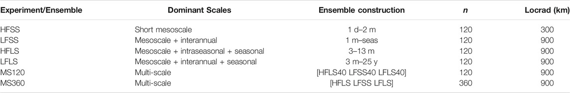
TABLE 1. Summary of experiments, including the name of each experiment/ensemble, descriptors of the dominant spatiotemporal scales represented, details of the ensemble construction, ensemble size (n)m and localosation radius (LOCRAD, in km). Under ensemble construction, d, m, and y refer to days, months, and years; and Seas is seasonal climatology; and describe how ensemble members are constructed. For example, 1 d–2 m, means 1-day minus 2 month centered-averages; 3–13 m, means 3 month centered-average minus a 13-month centered-average. For each 120-member ensemble, four members are calculated for each year, using fields from 30 years of a 35-year model run. For MS120, 40 members from each of the child ensembles (HFLS, LFSS, and LFLS) are used. The localisation radius refers to the distance over which the localising function reaches zero.

The standard deviation of the salinity anomalies at 250 m depth are shown for each 120-member ensemble in Figure 1. This field quantifies the assumed background field error for the EnOI system. The most salient aspect of this comparison is the difference in amplitude of the standard deviations, with much larger values for LFSS and LFLS, compared to HFSS and HFLS. Both HFSS and HFLS also include vast regions of very small values. In those regions of very small assumed background field errors, the assimilation of salinity observations may have only a small impact. In the limit that we assume the background field error is zero—assimilation of data will have no impact at all (because we assume the background field is perfect). The average value for the HFSS, LFSS, HFLS, and LFLS ensemble for salinity at 250 m depth is 0.02, 0.06, 0.03, and 0.06 psu respectively. Because LFSS and LFLS assume a larger background field error, using the same observation error estimates, the experiments with these ensembles should (in theory) “fit” the observations more closely than the experiments using the HFSS and HFLS ensemble. In practice, as discussed above, this also depends on whether the anomalies in each ensemble are well-suited to “fit” the background innovations (from Eq. 2).

FIGURE 1

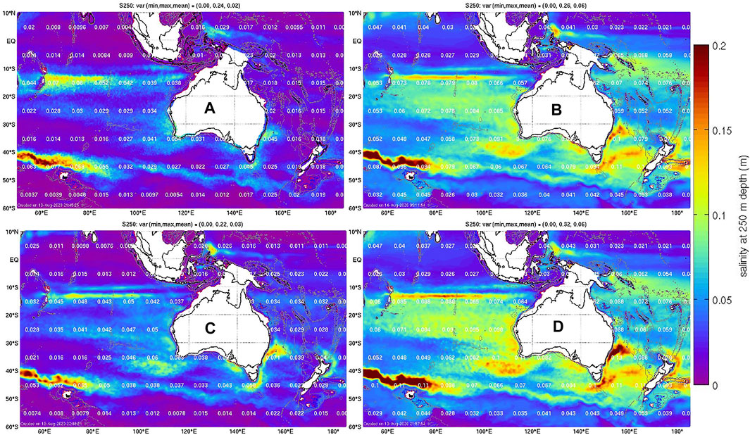
FIGURE 1. Standard deviation of the anomalies (ensemble spread) of salinity at 250 m depth for the (A) HFSS, (B) LFSS, (C) HFLS, and (D) LFLS ensemble. The white numbers overlaying the coloured fields report the 10 × 10° average for the standard deviation for each area.

Examples of the anomalies for temperature at 250 m depth, showing the first three ensemble members for each ensemble, are presented in Figure 2. Several differences between the ensembles are immediately evident. Like the standard deviations for salinity at 250 m depth, the amplitudes of anomalies for temperature at 250 m depth are much smaller in the HFSS and HFLS ensembles compared to the LFSS and LFLS ensembles. This is because the HFSS and HFLS do not include anomalies associated with interannual variability. All of the ensembles include anomalies that we might associate with eddies—showing many positive and negative anomalies on eddy-scales in eddy-rich regions. Close inspection shows that the mesoscale features are smallest in the HFSS ensemble, compared to the other ensembles. The LFSS and LFLS ensembles include zonal bands of significant anomalies, between 20–30°S and 40–50°S, and broad regions of non-zero anomalies at low latitudes. We associate these bands of anomalies with interannual variability. The HFLS ensemble includes some zonal bands of anomalies, with smaller amplitude, between about 40 and 10°S, that we interpret as seasonal anomalies.

FIGURE 2

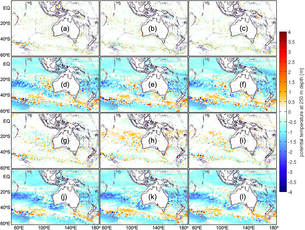
FIGURE 2. Examples of anomalies from the first three ensemble members for the (A–C) HFSS ensemble, (D–F) LFSS ensemble, (G–I) HFLS ensemble, and the (J–L) LFLS ensemble.

Based on the salient characteristics evident in Figures 1, 2, we might expect quite different results using HFSS compared to LFSS, HFLS, and LFLS; and we equally might expect many differences between LFSS compared to HFLS and LFLS.

The length-scales evident in the ensemble fields are also used to guide the localisation length-scales (Table 1). For HFSS, the length-scales are short, and so we only test the system using a length-scale of 300 km (with an effective e-folding length-scale of about 100 km). For LFSS, HFLS, LFLS, M120, and MS360, the anomalies in the ensemble include broader-scale features. These ensembles may warrant length-scales exceeding 1,000 or even 2000 kms. Here, we’re constrained by computational resource, and we settle for experiments with a localisation length-scale of 900 km (with an effective e-folding length-scale of about 300 km). Additionally, Figure 2 also shows that the length-scales in HFLS and significantly shorter than LFSS and LFSS. This suggests that there may be some benefit in using different length-scales for different ensemble members in the MS120 and MS360 experiments. Unfortunately, this is option is not available in EnKF-C (Sakov, 2014), but we note that scale-dependent localisation has been used in the context of four-dimensional ensemble-variational data assimilation for Numerical Weather Prediction (e.g., Buehner and Shlyaeva, 2015; Caron and Buehner, 2018).

3 Results

3.1 Comparisons with Assimilated Data

Blue Maps has been run for six different experiments (Table 1) to produce weekly analyses over a 4-year period (1/2015–12/2018). Time series of the mean absolute difference (MAD) between observations and analyses (analysis innovations) and observations and background fields (background innovations) for each experiment are presented in Figure 3. This shows the global average for each variable using data within 3 days of each analysis. The averages in both time and space are shown in Table 2 for background and analysis innovations.

FIGURE 3

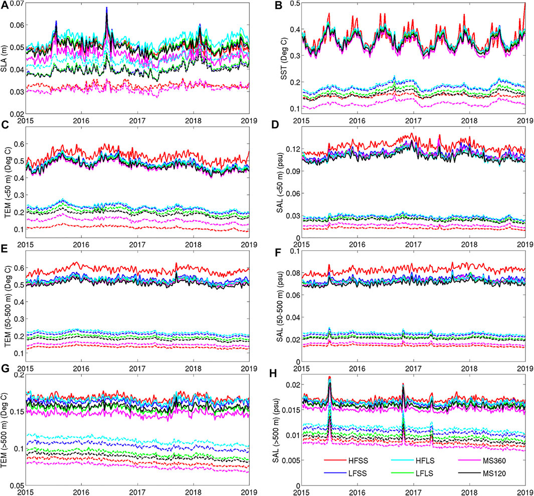
FIGURE 3. Time-series of MAD between observations and analyses (dashed lines) and background fields (solid lines) for different experiments, for observations within 3 days of each analysis. Results are shown for (A) SLA, (B) SST, and (C, E, G) temperature and (D, F, H) salinity for different depth ranges, as labeled on the vertical axes. The legend for different experiments is shown in panel (H).

TABLE 2

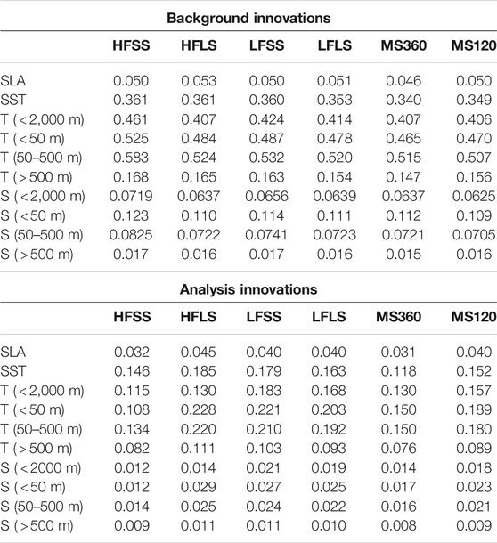
TABLE 2. Time-average of the global MAD between observations and background fields (top group; titled background innovations)) and between observations and analysis fields (bottom group, titled analysis innovations), for observations within 3 days of each analysis (a 6 days time-window) for SLA (m), SST (°C), temperature (T, °C) and salinity (S, psu). Metrics for T and S are shown for all depths shallower than 2000 m, for 0–50 m, 50–500 m, and 500–2000 m.

The results in Figure 3 show that the system’s performance for all experiments is relatively stable. There are a few points in time with unusually large innovations. For SLA, there appears to be one of two times when there is large background innovations (e.g., mid-2015, and mid-2016); and for salinity below 500 m depth, there are three times when the innovations spike (mid-2015, late-2016, and early-2017). We expect that these anomalies are caused by assimilation of bad data.

For SLA and upper-ocean fields, Figure 3 shows that there is a seasonal cycle in the performance, with analysis and background innovations slightly larger in austral winter. For deep temperature and salinity, the innovations also show a small, quasi-linear reduction in time.

For SLA, smallest analysis innovations are found in HFSS and MS360, indicating that analyses fit the observed SLA equally well for both experiments. But the background innovations are notably larger for HFSS compared to MS360. This indicates that although the analyses in HFSS fit the observations with similar accuracy to MS360, it seems that HFSS includes some unrealistic features that result in larger differences with the next background field. We interpret this as a case of over-fitting in HFSS, and attribute this to the small length-scales in the HFSS ensemble (Figure 2) and the short localisation length-scale used for the HFSS experiment (Table 1). This result for SLA, is similar to other variables, where HFSS analysis innovations are most similar to MS360 of all the experiments, but with HFSS consistently producing the largest background innovations. This is most clear for temperature and salinity in the depth ranges of 0–50 m and 50–500 m (Figure 3). For these metrics, the HFSS analysis innovations are the smallest of all experiments - providing analyses with the best fit to observations—but the HFSS background fields are the largest of all experiments—providing analyses with the worst fit to observation of the experiments presented here. These metrics are quantified in Table 2, where the HFSS analyses show the smallest analysis innovations, but the largest background innovations for most variables.

Weighing up both the analysis and background innovations reported in Figure 3 and in Table 2, we conclude that the best performing experiment is clearly MS360. It’s interesting that MS360 outperforms the child ensembles of LFSS, HFLS, and LFLS for every metric. It is also worth noting that for most metrics, MS120 outperformed LFSS, HFLS, and LFLS, leading us to conclude that the diversity of anomalies in the multi-scale ensemble experiments is beneficial. Furthermore, we find that MS360 outperformed MS120 on all metrics, demonstrating the benefit of increased ensemble size. We will explore why this is the case below, in Section 4.

Profiles of MAD for temperature and salinity innovations are presented in Figure 4, showing averages over the entire globe, and for each basin for the MS360 experiment only. Figure 4 includes both profiles for MAD for analysis and background innovations. For both temperature and salinity, the analysis innovations for MS360 are small, showing mis-fits to gridded observations of less than 0.1°C for temperature for most depths, and less than 0.01 psu for salinity for most depths. For context, recall that the assumed observation errors for in situ temperature and salinity are 0.05°C and 0.05 psu, respectively. For the background innovations for temperature (Figure 4A), the MAD is largest at around 100 m depth, the average depth of the thermocline. The largest background innovations in the upper ocean are in the Indian Ocean and the equatorial and South Atlantic Ocean. Below about 200 m depth, the largest background innovations are in the North Atlantic Ocean. For salinity profiles (Figure 4B), the MAD is largest at the surface for most regions, with the largest mis-fits in the Atlantic and Indian Oceans. Like temperature, the largest background innovations below about 300 m depth are in the North Atlantic Ocean. The smallest background innovations for salinity are in the upper ocean are in the Southern Ocean.

FIGURE 4

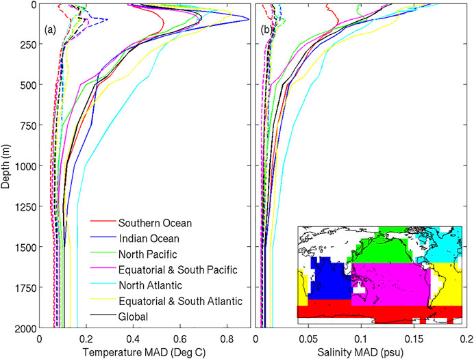
FIGURE 4. Profiles of MAD between observations and analyses (dashed lines) and observations and background fields (solid lines) for (A) temperature and (B) salinity. Profiles are shown for different regions (coloured lines) and for the global average (black). The inset in panel (B) shows the regional partitioning. Results are for the MS360 experiment. Only observations made within 2 days of each analysis time are included in these calculations.

Maps of the MAD of background and analysis innovations for SLA and SST are presented in Figure 5 for MS360. As expected, the largest innovations for SLA are in the eddy-rich regions, namely the western boundary current (WBC) extensions and along the path of the Antarctic Circumpolar Current (ACC). SLA innovations are also larger off Antarctica, where there are fewer SLA observations. For SST, there are also local maxima of innovations in each WBC region; and there are larger values north of about 30°S, with the largest values at the northern-most latitudes of the grid.

FIGURE 5

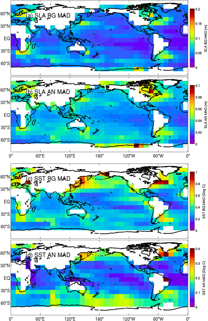
FIGURE 5. Map of the MAD between (A,C) observations and background fields (BG; 7 days after each analysis), and between (B,D) observations and analyses (AN) for (A,B) SLA and (C,D) SST. Results are for the MS360 experiment. Only observations made within 2 days of each analysis time are included in these calculations.

Maps of the MAD of background and analysis innovations for temperature and salinity at depths of 10, 100, 200, and 1,000 m depth are presented in Figures 6 and 7, respectively for MS360. The maps for temperature and salinity at corresponding depths show similar structures, with local maxima and minima in approximately the same regions. At 10 m depth, the largest innovations are in the WBC regions and in the eastern Tropical Pacific. At 100 m depth, in addition to larger values in WBCs, there are also larger values for all longitudes in the tropical bands for each basin. This is where the pycnocline has the strongest vertical gradient, and so any mis-placement of analysed isopycnal depths has a large penalty for MAD of temperature and salinity. At 200 m depth, there is evidence of a band of higher innovations nearer the center of each ocean basin at mid-latitudes. For the South Pacific, this band of higher innovations may relate to the decadal variability identified by O’Kane et al. (2014). At 1,000 m depth, the innovations are small everywhere, with modest local maxima in WBC regions.

FIGURE 6

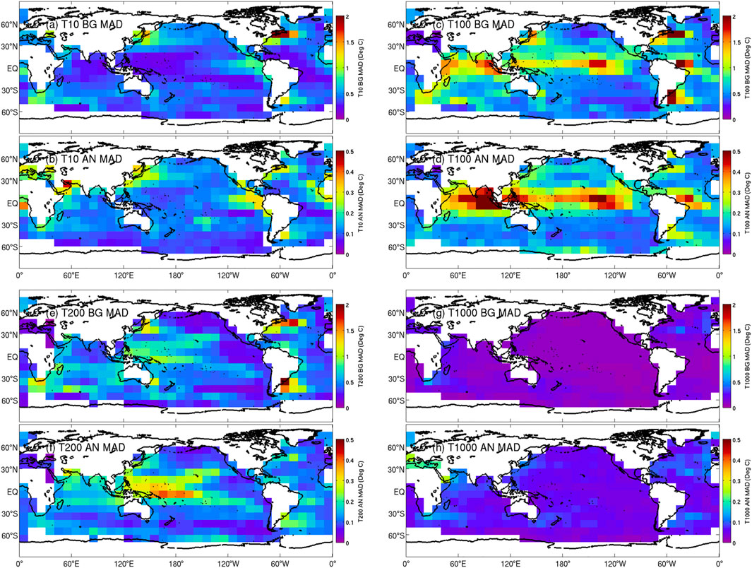
FIGURE 6. Map of the MAD between (A,C,E,G) observations and background fields (7 days after each analysis), and between (B,D,F,H) observations and analysis fields, for temperature at (A,B) 10 m, T10; (C,D) 100 m, T100; (E,F) 200 m, T200; and (G,H) 1,000 m depth, T1000. Results are for the MS360 experiment. Only observations made within 2 days of each analysis time are included in these calculations.

FIGURE 7

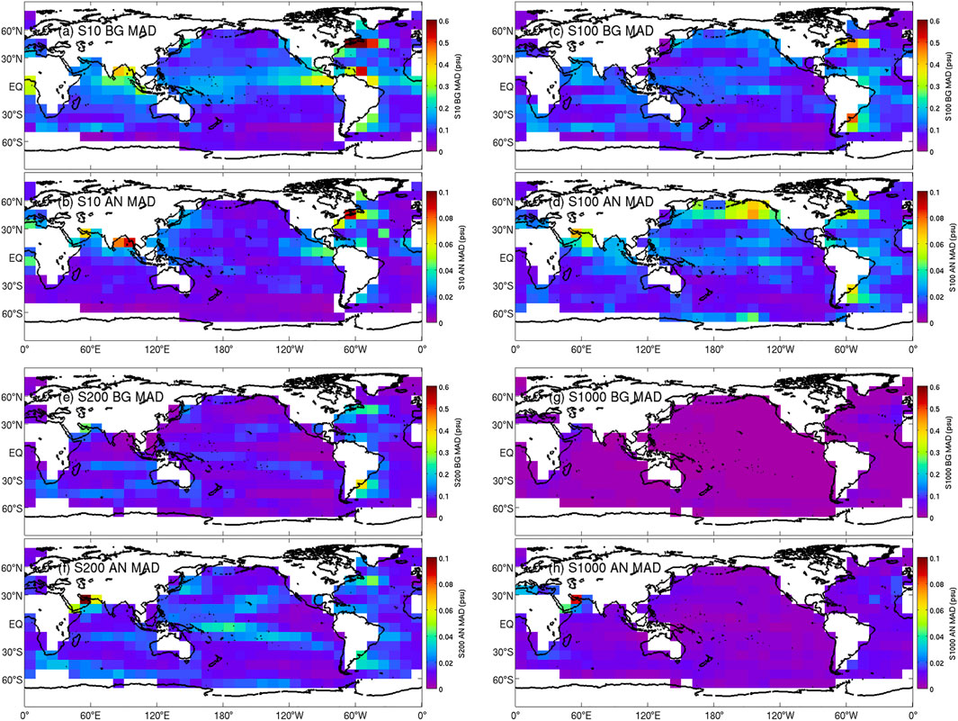
FIGURE 7. As for Figure 6, except for salinity.

3.2 Comparisons with Independent Data

For the comparisons presented above, the analyses of the background innovations can be considered as independent validation, since this involves comparisons between Blue Maps analyses and observations that have not been used to construct an analysis. However, for the comparisons of in situ temperature and salinity, the observations are mostly from Argo floats. Because Argo floats drift slowly, this means that the “independent” comparisons (based on the background innovations) almost always involves comparisons between background fields with observations in locations where data was recently assimilated. As a result, we might suspect that these comparisons provide an optimistic assessment of the accuracy of the analysis system. We therefore seek an additional, truly independent assessment here.

For an independent assessment, we compare analyses of temperature and salinity with non-Argo data from eXpendable BathyThermographs (XBTs; temperature only), Conductivity-Temperature-Depth (CTD) measurements from ship-borne surveys, moorings (mostly the tropical mooring arrays), and from sensors mounted on marine mammals (mostly in the Southern Ocean, near the Kerguelen Plateau). We source these data from the Coriolis Ocean Dataset for ReAnalysis CORA (CORA, versions 5.0 and 5.1; Cabanes et al., 2013). The global-averaged profiles of the MAD for 1/2015–12/2017 (CORA data are not currently available post-2017) are presented in Figure 8. For temperature, this mostly includes data from sensors mounted on marine mammals in the Indian Ocean section of the Southern Ocean, the tropical mooring arrays, and a small number of XBT transects and CTD surveys (Figure 8A). For salinity, this is mostly marine mammals and the tropical moorings. The coverage of non-Argo data for this comparison is not truly global, with vast amounts of the ocean without any non-Argo data available. Despite the poor coverage, this comparison provides some assessment against truly independent observations. This comparison indicates that the differences between Blue Maps analyses and non-Argo (independent) observations are about the same amplitude as the background innovations, presented in Figure 4—slightly higher for salinity. This indicates that misfits with independent data for temperature are largest at about 100 m depth, with values of about 0.8°C; and for salinity are largest at the surface, with value of about 0.3 psu.

FIGURE 8

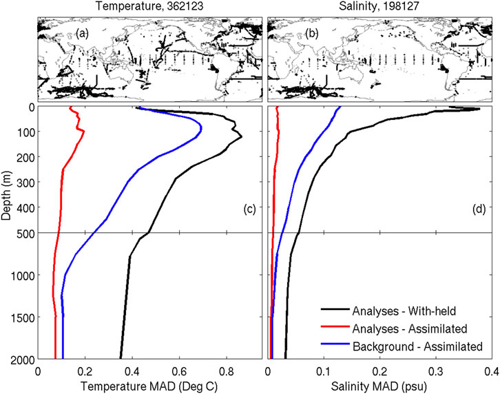
FIGURE 8. Profiles of global-averaged MAD between analyses (from MS360) and non-Argo with-held observations (black), analyses and assimilated observations (red), and background fields and assimilated observations (blue), for (C) temperature and (D) salinity, from 1/2015–12/2017. The top panels show the locations of non-Argo (A) temperature and (B) salinity observations; and the numbers in the title are the number of respective observations. The non-Argo data includes XBT (temperature only) and CTD; plus sensors on marine mammals (MAM) and moorings (MOR).

Considering the analysis innovations reported in Table 2 and presented in Figures 3–8, we conclude that the gridded estimates of ocean temperature, salinity, and sea-level in Blue Maps have comparable accuracy to observation-based products. Here, we summarise the estimated errors and data-misfits reported elsewhere in the literature for a widely-used gridded SLA product (Pujol et al., 2016), SST product (Good et al., 2020), and temperature and salinity product (Roemmich and Gilson, 2009). For SLA, Pujol et al. (2016) report that the standard deviation of error of a 1/3°-resolution gridded SLA product (DUACS DT2014) ranges from 2.2 cm in low-variability regions, to 5.7 cm in high-variability regions (their Table 2). For SST, Good et al. (2020) show that the misfits between gridded SST and Argo match-ups to range from about 0.3 and 0.5°C between 2015–2018 (their Figure 11). For sub-surface temperature, Li et al. (2017) report that misfits between gridded temperature (for Roemmich and Gilson, 2009) and independent in situ data from tropical moorings average about 0.5°C, with largest misfits of about 0.8°C at 100 m depth (the surface) and about 0.2°C at 500 m depth (their Figure 9). For salinity, Li et al. (2017) report that misfits between gridded salinity (for Roemmich and Gilson, 2009) and independent in situ data from tropical moorings average about 0.1 psu, with largest misfits of about 0.2 psu at the surface and about 0.02 psu at 500 m depth (their Figure 10). For each gridded variable, the reported accuracy of these observational products are comparable to the accuracy of Blue Maps analysis fields. We therefore maintain that the accuracy of Blue Maps analyses is comparable to other widely-used observation-based products.

3.3 Example Analyses

To demonstrate the scales represented by Blue Maps analyses, we show some examples of anomalies of sea-level, temperature, and salinity in Figures 9, 10. These examples demonstrate the abundance and amplitude of mesoscale variability in the maps. Anomalies that are obviously associated with eddies are evident in the SLA fields (Figures 9A, 10A) throughout most of the regions displayed. Signals of these eddies are also clearly evident in the anomalies at 250 m depth, and in some regions (e.g., along the path of the ACC—particularly near the Kerguelen Plateau, Figures 9D,E; and in the eddy-rich parts of the Tasman Sea, Figures 10D,E). Regions of broad-scale anomalies are also evident, including high sea-level, and cold and fresh anomalies in the western, equatorial Pacific (Figures 9A–C). The maps also show deep salinity anomalies at 1,000 m depth between 20 and 30°S in the Indian Ocean, and along the path of the ACC (Figure 9). Of course, the anomalies displayed here are on depth levels, and so the relative contributions from heaving of the water column and changes in ocean properties from climatology are unclear. Assessment of this aspect of the analyses is important and interesting, but is not addressed in this study.

FIGURE 9

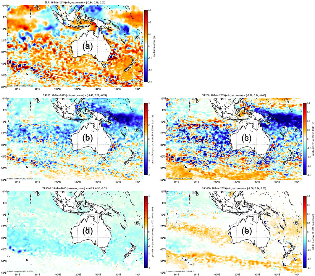
FIGURE 9. Examples of gridded fields from MS360, showing anomalies of (A) sea-level, (B) temperature at 250 m depth, (C) salinity at 250 m depth, (D) temperature at 1,000 m depth, and (E) salinity at 1,000 m depth. Fields are shown for March 16, 2015. The title of each panel reports the minimum, maximum, and mean of the field displayed. Anomalies are with respect to seasonal climatology from WOA13 (Locarnini et al., 2013; Zweng et al., 2013) and the mean sea-level field from OFAM3 (Oke et al., 2013b).

FIGURE 10

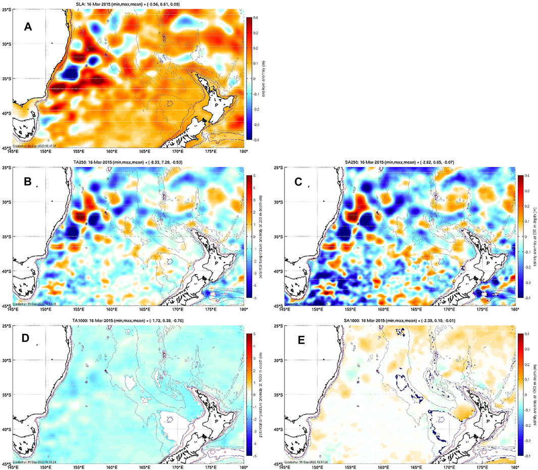
FIGURE 10. As for Figure 9, except for the tasman sea.

4 Analysis and Discussion

4.1 Understanding the Performance of the MS360 Ensemble

An exciting and intriguing result reported in Section 3 is the superior performance of MS360 compared to LFSS, HFLS, and LFLS—the child ensembles. In this case, the performance of the larger parent ensemble (MS360) is not just marginally better than each of the child ensembles—the difference is quite significant—particularly for the analysis innovations. For many metrics, the MAD for the analysis innovations are up to 30–35% smaller in MS360, the child ensemble experiments (22–36% smaller for salinity at 50–500 m depth, for example, Table 2). Here, we seek to understand why the experiment with the MS360 ensemble performs so much better. Based on comparisons between the innovations reported in Figure 3 and in Table 2, we suggested above that both the ensemble size and the diversity of anomalies in the multi-scale analyses are important. We aim to explore this further below.

To understand how the MS360 experiment uses ensemble members from each of the child ensembles, we analyse the ensemble weights (from Eq. 2) for 52 analyses—one for each week—during 2015. We then calculate the fraction of the increment that can be attributed to each child ensemble by calculating a partial sum of the weighted ensemble members (from Eq. 2), using only the members for each child ensemble. We show a map of the average fraction of increment explained by each child ensemble for temperature at 250 m depth, and also present the zonally-averaged profiles, in Figure 11. The results show that in different regions, each child ensemble is given a different relative weight. For all examples in Figure 11, anomalies in LFLS are combined to produce the largest fraction (about 60$\text{\%}$) of the increments for almost all latitudes. We show that anomalies from LFSS are dominant in each WBC region, where there is correspondingly low weight assigned to anomalies from LFLS. This provides a clear indication that different types of ensembles are warranted in different dynamical regimes. Another example of this is in the South Pacific, where there is a band of high values for LFLS extending from the southern tip of South America and extending towards central eastern Australia. Although not perfectly aligned, this is reminiscent of the path of quasi-decadal anomalies identified by O’Kane et al. (2014). There are also different bands where HFLS has relatively higher weight—particularly at low latitudes in the Pacific and Atlantic Oceans, and along the path of the ACC south of Australia. This analysis provides a detailed and complex picture of the relative weights assigned by the EnOI system to each child ensemble. The key message we take away from this analysis, is that different types of anomalies are assigned different weights in different regions.

FIGURE 11

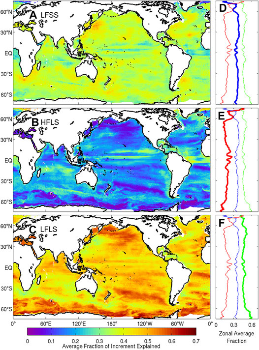
FIGURE 11. Average fraction of increment explained for temperature at 250 m depth, for each child ensemble, including (A) LFSS, (B) HFLS, and (C) LFLS, in the MS360 experiment. The zonal averages for LFSS (blue), HFLS (red), and LFLS (green) are shown in panels (D–F). Averages are calculated from 52 analyses during 2015.

The analysis of the relative fraction of increment explained by each child ensemble in MS360 (Figure 11), confirms that the relative weights of the anomalies in the different child ensembles varies for different dynamical regimes. This result has a number of implications. Recall that EnOI requires an explicit assumption about the background field errors. Specifically, the construction of the stationary ensemble for EnOI requires the ensemble to be generated by constructing anomalies for some space- and time-scales—here summarised in Table 1 (column three therein). Almost all applications of EnOI in the literature invoke a single assumption about the background error covariance to construct the ensemble. The only exceptions that we are aware of are presented by Cheng and Zhu (2016), Cheng et al. (2017), and Yu et al. (2019). Here, we show that we achieve a much better result when several different assumptions are made together, and a diversity of ensemble members are combined to construct analyses. Moreover, the results presented here indicate that a different assumption about the background field errors is warranted for different regions.

Another element of Blue Maps that differs from most other applications of EnOI is the use of longer localisation length-scales. For five of the experiments presented here, a 900 km localisation length-scale is used (Table 1). To demonstrate the impact of this aspect of the configuration, we present examples of ensemble-based correlations between temperature at a reference location and nearby temperature, in Figure 12. To understand the impact of localisation, consider the profiles in Figure 12A, for example. For this case, the un-localised ensemble-based correlation (red) closely matches the localised ensemble-based correlation profile using a 900 km localisation function (green), but is significantly different from the localised ensemble-based correlation profile using a 250 km localisation function (blue). If the localisation function with the shorter length-scale is used, then the ensemble-based correlations are heavily modified. By contrast, if a localisation function with the longer length-scale is used, then the ensemble-based correlations are virtually un-modified within several hundred kilometres of the reference location. As a result, using the longer length-scales permits more of the structures—such as the anisotropy—of the ensemble-based correlations to be used for the data assimilation. Whereas, using the short length-scale localisation function, more of the details are eliminated, and the correlation used degrades towards a quasi-Gaussian function (like most objective analysis systems). In this way, some of the benefits of EnOI are lost when a shorter length-scale is used. The other examples presented in Figure 12 demonstrate the same relationships. We have looked at equivalent fields to these for many other regions. The results in Figure 12 are similar to many regions poleward of about 15°N and S. In the equatorial region, the unlocalised correlations are much longer (several thousand kilometres in some cases). For those tropical regions, a longer localisation length-scale is warranted—but we cannot afford to implement this computationally, due to memory requirements, to assess the performance.

FIGURE 12

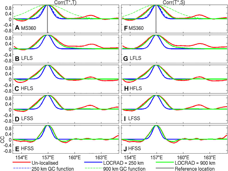
FIGURE 12. Ensemble-based correlations between temperature at 250 m depth at 32°S and 157°E in the Tasman Sea, and temperature and salinity at the same depth and longitude, but at nearby longitudes using different ensembles: (A,F) MS360, (B,G) LFLS, (C,H) HFLS, (D,I) LFSS, and (E,J) HFSS. Each panel includes the un-localised ensemble-based correlation (in red), the localised ensemble-based correlation, multiplied by the 250 km localisation function (blue) and multiplied by the 900 km localisation function (green). Also shown in panels (A) and (F) are the correlations functions with a 250 km (blue-dashed) and 900 km (green-dashed) using the formulation used here and defined by Gaspari and Cohn (1999). The location of the reference point is also shown in panels (A) and (F) with a vertical grey line.

4.2 Development Experiments

The development of Blue Maps has involved a large number of trial experiments that produced mixed results. Not all of the results from this series of experiments can be reported here in detail. But some of the findings from those experiments will be summarised here, since they may be of interest to the community. The first configuration of Blue Maps used the same configuration as the 2016 version of BRAN (Oke et al., 2018). This was similar to the HFSS experiment reported here. However the HFSS experiment includes a few modifications. Early results used persistence for the background field—not damped persistence (Eq. 4). The quality of the analyses degraded in time, with noisy fields emerging and growing in amplitude. It appears that there are insufficient observations to constrain a series of analyses without damped persistence and without an under-pinning model. Damped persistence was adopted thereafter. Many experiments were performed with damping to climatology using an e-folding time-scale in the range of 7–90 days. The best overall performance—based on the analysis and background innovations—was found using damping with an e-folding time-scale of 14-days. This time-scale is used in all experiments described in this paper. Damped persistence is commonly used for SST analyses. For example, the Operational Sea Surface Temperature and Sea Ice Analysis (OSTIA), produced by the UKMet Office, uses damped persistence with an e-folding timescale of 30 days for ice-free regions (Donlon et al., 2012; Fiedler et al., 2019; Good et al., 2020). Similarly, the operational SST analysis produced by the Canadian Meteorological Centre (CMC) uses damped persistence with an e-folding timescale of 58 days (Brasnett, 2008; Brasnett and Colan, 2016).

Even using damped persistence, small-scale noise still appeared in analyses in some regions. Close examination of the ensemble fields showed that there were noisy fields in most ensemble members. As a consequence, these noisy features appear in the analyses, according to Eq. 2. We eliminated these small-scale features by spatially smoothing of the ensemble fields. This was implemented here (for all ensembles) using a simple horizontal diffusion operator (that applies a spatial smoothing with a footprint of 1x1°). We now understand that a similar approach to smooth the ensemble has long be used for the French ocean reanalysis, as reported by Artana et al. (2019), for GLORYS (the GLobal Ocean ReanalYses and Simulations).

Other experiments explored the sensitivity to localisation length-scale. The results with longer length-scales generally performed better, with fewer fictitious features that are not resolved by the observations. Computational limitations prohibited us from testing the system with longer length-scales.

Some of the lessons learnt during the development of Blue Maps may be of interest to the ocean data assimilation community. Apparently many of the features identified in the early experiments during this development are present in BRAN experiments (e.g., small-scale noise in analyses). But it appears that when fields with these artefacts are initialised in a model, the model efficiently disperses many of the artificial features, and they are not clearly evident in the resulting reanalysis fields (which are often daily-means). Surely, inclusion of these fictitious features - albeit small in amplitude—will degrade the quality of ocean reanalyses. For Blue Maps, these features were easily identified, because there is no model to “cover” over the unwanted features. We plan to apply the learnings from the development described here, to future versions of BRAN.

5 Conclusion

A new observation-based product that adapts a data assimilation system that has traditionally been used for ocean forecasting and ocean reanalysis is presented here. The new product is called Blue maps. Blue Maps is tested here by producing weekly analysis over a 4-year period (1/2015–12/2018). We compare the performance of Blue Maps for six different configurations, using different ensembles. The best performance is achieved using a 360-member multi-scale ensemble (MS360) that includes anomalies from several different spatiotemporal scales. For that configuration, analyses of sea-level that are within about 4 cm of observations; and analyses of upper-ocean (deep) temperature and salinity that are within about 0.45 (0.15) degrees and 0.1 (0.015) psu respectively. These misfits are comparable to ocean reanalysis systems that are underpinned by an ocean model. For example, the 2020 version of the Bluelink ReANalysis (BRAN 2020, Chamberlain et al., 2021a), fits data to within about 0.17–0.45°C and 0.036–0.082 psu (smallest values are for misfits of observations and analysis; largest values are misfits of observations and 3 days “forecasts”). GLORYS12V1 (Lellouche et al., 2019, see their Figure 5B), version 2020, fits the data to within about 0.41°C and 0.061 psu. For equivalent metrics, Blue Maps fits data to within 0.17–0.41°C and 0.014–0.064 psu (smallest values are for misfits of observations and analysis; largest values are misfits of observations and 7 days “damped persistence”). Compared to observation-based products, Blue Maps also compares well. Li et al. (2017) present results from a 1°-resolution product and includes an inter-comparison with other observation-based products. They show that their system performs comparably to analyses produced by Roemmich and Gilson (2009), and a number of other coarse-resolution products. The profiles of analysis-observation misfits in Figure 4, for Blue Maps, show much smaller mis-fits than observational products presented by (Li et al., 2017, e.g., their Figure 4).

We show that the superior performance of the Blue Maps configuration using the ensemble with multiple spatiotemporal scales is because of the larger ensemble size (120 compared to 3,670), longer length-scales (compared to most other EnOI applications), and the diversity of ensemble anomalies. We conclude that different assumptions about the system’s background error covariance are warranted for different regions. We recognise that the ensemble with 360 members—although larger than most other global applications of EnOI—is still not large. Indeed, the most extreme demonstration of the benefits of a truly large ensemble is presented by Miyoshi et al. (2015), who presented some very impressive results using a 10,240-member ensemble for numerical weather prediction. We suspect further improvements may be achieved if a larger, more diverse ensemble is used. This suggestion will be explored in future experiments with Blue Maps and with BRAN. Future developments of Blue Maps will also likely include explicit analyses of mixed layer depths, biogeochemical parameters (e.g., backscatter), and will include a calculation of weekly fields for a longer period (probably from 2000 to present).

Data Availability Statement

The datasets presented in this study can be found in online repositories. The names of the repository/repositories and accession number(s) can be found below: https://dapds00.nci.org.au/thredds/catalog/gb6/BRAN/Blue_Maps/MAPS-v1p0/catalog.html.

Author Contributions

PO conceived and designed the study, performed the calculations, the analysis, and wrote the first draft of the manuscript. MC contributed to the design of the study, development of scripts for producing the analysis system, and organised the observational database. RF prepared some of the ensembles and contributed to the development of scripts for producing the analysis system. HuB developed the first version of system analysis here. HuB developed the first version of the analysis system described here. GB provided important input to the design of the study. All authors contributed to manuscript revision, read, and approved the submitted version.

Funding

Funding for this research has been received from IMOS and Bluelink, including funding from CSIRO, BoM, and the Australian Department of Defence.

Conflict of Interest

The authors declare that the research was conducted in the absence of any commercial or financial relationships that could be construed as a potential conflict of interest.

Acknowledgments

The authors gratefully acknowledge support from IMOS: a national collaborative research infrastructure, supported by the Australian Government; the Bluelink Partnership: a collaboration between the Australian DoD, BoM and CSIRO; and the National Computational Infrastructure (NCI). Argo data were collected and made freely available by the International Argo Program: part of the Global Ocean Observing System. The AVHRR SST data was sourced from the Naval Oceanographic Office and made available under Multi-sensor Improved Sea Surface Temperature project, with support from the Office of Naval Research. NOAA and TU Delft are also gratefully acknowledged for the provision of RADS data. This study benefited from several constructive discussions with P. Sakov and S. Wijffels. The corresponding author also wishes to acknowledge the Edinburgh Gin Distillery for provision of Gin Liqueur that aided the writing of this paper.

Footnotes

¹argo.ucsd.edu/data/argo-data-products/.

References

Artana, C., Ferrari, R., Bricaud, C., Lellouche, J.-M., Garric, G., Sennéchael, N., et al. (2019). Twenty-five Years of Mercator Ocean Reanalysis GLORYS12 at Drake Passage: Velocity Assessment and Total Volume Transport. Adv. Space Res. doi:10.1016/j.asr.2019.11.033

CrossRef Full Text | Google Scholar

Balmaseda, M. A., Mogensen, K., and Weaver, A. T. (2012). Evaluation of the ECMWF Ocean Reanalysis System ORAS4. Q.J.R. Meteorol. Soc. 139, 1132–1161. doi:10.1002/qj.2063

CrossRef Full Text | Google Scholar

Balmaseda, M. A., Hernandez, F., Storto, A., Palmer, M. D., Alves, O., Shi, L., et al. (2015). The Ocean Reanalyses Intercomparison Project (ORA-IP). J. Oper. Oceanogr. 8, s80–s97. doi:10.1080/1755876x.2015.1022329

CrossRef Full Text | Google Scholar

Brasnett, B., and Colan, D. S. (2016). Assimilating Retrievals of Sea Surface Temperature from VIIRS and AMSR2. J. Atmos. Oceanic Technol. 33, 361–375. doi:10.1175/jtech-d-15-0093.1

CrossRef Full Text | Google Scholar

Brasnett, B. (2008). The Impact of Satellite Retrievals in a Global Sea-Surface-Temperature Analysis. Q.J.R. Meteorol. Soc. 134, 1745–1760. doi:10.1002/qj.319

CrossRef Full Text | Google Scholar

Brassington, G. B., Pugh, T. F., Spillman, C., Schulz, E., Beggs, H., Schiller, A., et al. (2007). Bluelink Development of Operational Oceanography and Servicing in Australia. J. Res. Pract Inf Tech 39, 151–164.

Google Scholar

Buehner, M., and Shlyaeva, A. (2015). Scale-dependent Background-Error Covariance Localisation. Tellus A: Dynamic Meteorology and Oceanography 67, 28027. doi:10.3402/tellusa.v67.28027

CrossRef Full Text | Google Scholar

Cabanes, C., Grouazel, A., von Schuckmann, K., Hamon, M., Turpin, V., Coatanoan, C., et al. (2013). The CORA Dataset: Validation and Diagnostics of In-Situ Ocean Temperature and Salinity Measurements. Ocean Sci. 9, 1–18. doi:10.5194/os-9-1-2013

CrossRef Full Text | Google Scholar

Caron, J.-F., and Buehner, M. (2018). Scale-dependent Background Error Covariance Localization: Evaluation in a Global Deterministic Weather Forecasting System. Monthly Weather Rev. 146, 1367–1381. doi:10.1175/mwr-d-17-0369.1

CrossRef Full Text | Google Scholar

Carton, J. A., and Giese, B. S. (2008). A Reanalysis of Ocean Climate Using Simple Ocean Data Assimilation (SODA). Monthly Weather Rev. 136, 2999–3017. doi:10.1175/2007mwr1978.1

CrossRef Full Text | Google Scholar

Cayula, J. F., May, D., McKenzie, B., Olszewski, D., and Willis, K. (2004). A Method to Add Real-Time Reliability Estimates to Operationally Produced Satellite-Derived Sea Surface Temperature Retrievals. Sea Technol. 67–73.

Google Scholar

Chamberlain, M. A., Oke, P. R., Fiedler, R. A. S., Beggs, H., Brassington, G. B., and Divakaran, P. (2021a). Next Generation of Bluelink Ocean Reanalysis with Multiscale Data Assimilation: BRAN2020. Earth Syst. Sci. Data, submitted

Google Scholar

Chamberlain, M. A., Oke, P. R., Brassington, G. B., Sandery, P., Divakaran, P., and Fiedler, R. A. S. (2021b). Multiscale data assimilation in the Bluelink ocean reanalysis (BRAN). Ocean Modelling, submitted.

Google Scholar

Cheng, L., and Zhu, J. (2016). Benefits of Cmip5 Multimodel Ensemble in Reconstructing Historical Ocean Subsurface Temperature Variations. J. Clim. 29, 5393–5416. doi:10.1175/jcli-d-15-0730.1

CrossRef Full Text | Google Scholar

Cheng, L., Trenberth, K. E., Fasullo, J., Boyer, T., Abraham, J., and Zhu, J. (2017). Improved Estimates of Ocean Heat Content from 1960 to 2015. Sci. Adv. 3, e1601545. doi:10.1126/sciadv.1601545

PubMed Abstract | CrossRef Full Text | Google Scholar

Counillon, F., and Bertino, L. (2009). Ensemble Optimal Interpolation: Multivariate Properties in the Gulf of Mexico. Tellus A: Dynamic Meteorol. Oceanogr. 61, 296–308. doi:10.1111/j.1600-0870.2008.00383.x

CrossRef Full Text | Google Scholar

Dee, D. P., and Uppala, S. (2009). Variational Bias Correction of Satellite Radiance Data in the ERA-Interim Reanalysis. Q.J.R. Meteorol. Soc. 135, 1830–1841. doi:10.1002/qj.493

CrossRef Full Text | Google Scholar

Donlon, C. J., Martin, M., Stark, J., Roberts-Jones, J., Fiedler, E., and Wimmer, W. (2012). The Operational Sea Surface Temperature and Sea Ice Analysis (OSTIA) System. Remote Sens. Environ. 116, 140–158. doi:10.1016/j.rse.2010.10.017

CrossRef Full Text | Google Scholar

Evensen, G. (2003). The Ensemble Kalman Filter: Theoretical Formulation and Practical Implementation. Ocean Dyn. 53, 343–367. doi:10.1007/s10236-003-0036-9

CrossRef Full Text | Google Scholar

Ferry, N., Rémy, E., Brasseur, P., and Maes, C. (2007). The Mercator Global Ocean Operational Analysis System: Assessment and Validation of an 11-year Reanalysis. J. Mar. Syst. 65, 540–560. doi:10.1016/j.jmarsys.2005.08.004

CrossRef Full Text | Google Scholar

Fiedler, E. K., Mao, C., Good, S. A., Waters, J., and Martin, M. J. (2019). Improvements to Feature Resolution in the OSTIA Sea Surface Temperature Analysis Using the Nemovar Assimilation Scheme. Q.J.R. Meteorol. Soc. 145, 3609–3625. doi:10.1002/qj.3644

CrossRef Full Text | Google Scholar

Fu, W., She, J., and Zhuang, S. (2011). Application of an Ensemble Optimal Interpolation in a North/Baltic Sea Model: Assimilating Temperature and Salinity Profiles. Ocean Model. 40, 227–245. doi:10.1016/j.ocemod.2011.09.004

CrossRef Full Text | Google Scholar

Gaspari, G., and Cohn, S. E. (1999). Construction of Correlation Functions in Two and Three Dimensions. Q.J R. Met. Soc. 125, 723–757. doi:10.1002/qj.49712555417

CrossRef Full Text | Google Scholar

Good, S. A., Martin, M. J., and Rayner, N. A. (2013). En4: Quality Controlled Ocean Temperature and Salinity Profiles and Monthly Objective Analyses with Uncertainty Estimates. J. Geophys. Res. Oceans 118, 6704–6716. doi:10.1002/2013jc009067

CrossRef Full Text | Google Scholar

Good, S., Fiedler, E., Mao, C., Martin, M. J., Maycock, A., Reid, R., et al. (2020). The Current Configuration of the OSTIA System for Operational Production of Foundation Sea Surface Temperature and Ice Concentration Analyses. Remote Sens. 12, 720. doi:10.3390/rs12040720

CrossRef Full Text | Google Scholar

Guinehut, S., Dhomps, A.-L., Larnicol, G., and Le Traon, P.-Y. (2012). High Resolution 3-d Temperature and Salinity fields Derived from In Situ and Satellite Observations. Ocean Sci. 8, 845–857. doi:10.5194/os-8-845-2012

CrossRef Full Text | Google Scholar

Henderson, C. R. (1975). Best Linear Unbiased Estimation and Prediction under a Selection Model. Biometrics 31, 423–447. doi:10.2307/2529430

PubMed Abstract | CrossRef Full Text | Google Scholar

Ishii, M., Fukuda, Y., Hirahara, S., Yasui, S., Suzuki, T., and Sato, K. (2017). Accuracy of Global Upper Ocean Heat Content Estimation Expected from Present Observational Data Sets. Sola 13, 163–167. doi:10.2151/sola.2017-030

CrossRef Full Text | Google Scholar

Keppenne, C. L., and Rienecker, M. M. (2003). Assimilation of Temperature into an Isopycnal Ocean General Circulation Model Using a Parallel Ensemble Kalman Filter. J. Mar. Syst. 40-41, 363–380. doi:10.1016/s0924-7963(03)00025-3

CrossRef Full Text | Google Scholar

Kiss, A. E., Hogg, A. M., Hannah, N., Boeira Dias, F., Brassington, G. B., Chamberlain, M. A., et al. (2019). ACCESS-OM2: A Global Ocean-Sea Ice Model at Three Resolutions. Geosci. Model. Dev. Discuss. 2019, 1–58. doi:10.5194/gmd-2019-106

CrossRef Full Text | Google Scholar

Köhl, A., Stammer, D., and Cornuelle, B. (2007). Interannual to Decadal Changes in the ECCO Global Synthesis. J. Phys. Oceanogr. 37, 313–337. doi:10.1175/jpo3014.1

CrossRef Full Text | Google Scholar

Köhl, A. (2015). Evaluation of the GECCO2 Ocean Synthesis: Transports of Volume, Heat and Freshwater in the Atlantic. Q.J.R. Meteorol. Soc. 141, 166–181. doi:10.1002/qj.2347

CrossRef Full Text | Google Scholar

Lellouche, J.-M., Le Galloudec, O., Drévillon, M., Régnier, C., Greiner, E., Garric, G., et al. (2013). Evaluation of Global Monitoring and Forecasting Systems at Mercator Océan. Ocean Sci. 9, 57–81. doi:10.5194/os-9-57-2013

CrossRef Full Text | Google Scholar

Lellouche, J.-M., Greiner, E., Le Galloudec, O., Garric, G., Regnier, C., Drevillon, M., et al. (2018). Recent Updates to the Copernicus Marine Service Global Ocean Monitoring and Forecasting Real-Time 1∕12° High-Resolution System. Ocean Sci. 14, 1093–1126. doi:10.5194/os-14-1093-2018

CrossRef Full Text | Google Scholar

Lellouche, J., Legalloudec, O., Regnier, C., Levier, B., Greiner, E., and Drevillon, M. (2019). “Quality Information Document,” in Copernicus Marine Environmental Monitoring Service (CMEMS) (Toulouse, France: EU Copernicus Marine Service), 2 (1), pp81.

Google Scholar

Li, H., Xu, F., Zhou, W., Wang, D., Wright, J. S., Liu, Z., et al. (2017). Development of a Global Gridded Argo Data Set with Barnes Successive Corrections. J. Geophys. Res. Oceans 122, 866–889. doi:10.1002/2016jc012285

CrossRef Full Text | Google Scholar

Locarnini, R., Mishonov, A., Antonov, J., Boyer, T., Garcia, H., Baranova, O., et al. (2013). “World Ocean Atlas 2013, Volume 1: Temperature,” in NOAA Atlas NESDIS 74. Editors S. Levitus, and A. Mishonov (Washington, D.C.: U.S. Government Printing Office), 40.

Google Scholar

May, D. A., Parmeter, M. M., Olszewski, D. S., and McKenzie, B. D. (1998). Operational Processing of Satellite Sea Surface Temperature Retrievals at the Naval Oceanographic Office. Bull. Amer. Meteorol. Soc. 79, 397–407. doi:10.1175/1520-0477(1998)079<0397:oposss>2.0.co;2

CrossRef Full Text | Google Scholar

Miyoshi, T., Kondo, K., and Terasaki, K. (2015). Big Ensemble Data Assimilation in Numerical Weather Prediction. Computer 48, 15–21. doi:10.1109/mc.2015.332

CrossRef Full Text | Google Scholar

Naval Oceanographic Office (2014a). METOP-A AVHRR GAC L2P Swath SST Data Set. Ver. 1.0. PO.DAAC, CA, USA ,, Dataset Accessed 2017–01–01 to 2020–01–01 at. doi:10.5067/GHMTG–2PN02

CrossRef Full Text

Naval Oceanographic Office (2014b). METOP-B AVHRR GAC L2P Swath SST Data Set. Ver. 1.0. PO.DAAC, CA, USA , Dataset Accessed 2017–01–01 to 2020–01–01 at. doi:10.5067/GHMTB–2PN02

CrossRef Full Text

Naval Oceanographic Office (2014c). N-18 AVHRR GAC L2P Swath SST Data Set.Ver. 1.0. PO.DAAC, CA, USA , Dataset Accessed 2017–01–01 to 2020–01–01 at. doi:10.5067/GH18G–2PN02

CrossRef Full Text

Naval Oceanographic Office (2014d). N-19 AVHRR GAC L2P Swath SST Data Set. Ver. 1.0. PO.DAAC, CA, USA , Dataset Accessed 2017–01–01 to 2020–01–01 at. doi:10.5067/GH19G–2PN02

CrossRef Full Text

Ngodock, H. E., Jacobs, G. A., and Chen, M. (2006). The Representer Method, the Ensemble Kalman Filter and the Ensemble Kalman Smoother: A Comparison Study Using a Nonlinear Reduced Gravity Ocean Model. Ocean Model. 12, 378–400. doi:10.1016/j.ocemod.2005.08.001

CrossRef Full Text | Google Scholar

Ngodock, H., Souopgui, I., Carrier, M., Smith, S., Osborne, J., and D’Addezio, J. (2020). An Ensemble of Perturbed Analyses to Approximate the Analysis Error Covariance in 4dvar. Tellus A: Dynamic Meteorol. Oceanogr. 72, 1–12. doi:10.1080/16000870.2020.1771069

CrossRef Full Text | Google Scholar

O'Kane, T. J., Matear, R. J., Chamberlain, M. A., and Oke, P. R. (2014). ENSO Regimes and the Late 1970's Climate Shift: The Role of Synoptic Weather and South Pacific Ocean Spiciness. J. Comput. Phys. 271, 19–38. doi:10.1016/j.jcp.2013.10.058

CrossRef Full Text | Google Scholar

Oke, P. R., and Sakov, P. (2008). Representation Error of Oceanic Observations for Data Assimilation. J. Atmos. Oceanic Technol. 25, 1004–1017. doi:10.1175/2007JTECHO558.1

CrossRef Full Text | Google Scholar

Oke, P. R., Schiller, A., Griffin, D. A., and Brassington, G. B. (2005). Ensemble Data Assimilation for an Eddy-Resolving Ocean Model of the Australian Region. Q. J. R. Meteorol. Soc. 131, 3301–3311. doi:10.1256/qj.05.95

CrossRef Full Text | Google Scholar

Oke, P. R., Sakov, P., and Corney, S. P. (2007). Impacts of Localisation in the EnKF and EnOI: Experiments with a Small Model. Ocean Dyn. 57, 32–45. doi:10.1007/s10236-006-0088-8

CrossRef Full Text | Google Scholar

Oke, P. R., Brassington, G. B., Griffin, D. A., and Schiller, A. (2008). The Bluelink Ocean Data Assimilation System (BODAS). Ocean Model. 21, 46–70. doi:10.1016/j.ocemod.2007.11.002

CrossRef Full Text | Google Scholar

Oke, P. R., Brassington, G. B., Cummings, J., Martin, M., and Hernandez, F. (2012). GODAE Inter-comparisons in the Tasman and Coral Seas. J. Oper. Oceanogr. 5, 11–24. doi:10.1080/1755876x.2012.11020135

CrossRef Full Text | Google Scholar

Oke, P. R., Cahill, M. L., Griffin, D. A., and Herzfeld, M. (2013a). Constraining a Regional Ocean Model with Climatology and Observations: Application to the Hawaiian Islands. CAWCR Res. Lett. 20, 20–26.

Google Scholar

Oke, P. R., Griffin, D. A., Schiller, A., Matear, R. J., Fiedler, R., Mansbridge, J., et al. (2013b). Evaluation of a Near-Global Eddy-Resolving Ocean Model. Geosci. Model. Dev. 6, 591–615. doi:10.5194/gmd-6-591-2013

CrossRef Full Text | Google Scholar

Oke, P. R., Sakov, P., Cahill, M. L., Dunn, J. R., Fiedler, R., Griffin, D. A., et al. (2013c). Towards a Dynamically Balanced Eddy-Resolving Ocean Reanalysis: BRAN3. Ocean Model. 67, 52–70. doi:10.1016/j.ocemod.2013.03.008

CrossRef Full Text | Google Scholar

Oke, P. R., Griffin, D. A., Rykova, T., and de Oliveira, H. B. (2018). Ocean Circulation in the Great Australian Bight in an Eddy-Resolving Ocean Reanalysis: The Eddy Field, Seasonal and Interannual Variability. Deep Sea Res. Part Topical Stud. Oceanography 157-158, 11–26. doi:10.1016/j.dsr2.2018.09.012

CrossRef Full Text | Google Scholar

Oke, P. R. (2002). Assimilation of Surface Velocity Data into a Primitive Equation Coastal Ocean Model. J. Geophys. Res. 107, 1–25. doi:10.1029/2000JC000511

CrossRef Full Text | Google Scholar

Pujol, M.-I., Faugère, Y., Taburet, G., Dupuy, S., Pelloquin, C., Ablain, M., et al. (2016). Duacs Dt2014: the New Multi-mission Altimeter Data Set Reprocessed over 20 Years. Ocean Sci. 12, 1067–1090. doi:10.5194/os-12-1067-2016

CrossRef Full Text | Google Scholar

Ridgway, K. R., Dunn, J. R., and Wilkin, J. L. (2002). Ocean Interpolation by Four-Dimensional Weighted Least Squares-Application to the Waters Around Australasia. J. Atmos. Oceanic Technol. 19, 1357–1375. doi:10.1175/1520-0426(2002)019<1357:oibfdw>2.0.co;2

CrossRef Full Text | Google Scholar

Roemmich, D., and Gilson, J. (2009). The 2004-2008 Mean and Annual Cycle of Temperature, Salinity, and Steric Height in the Global Ocean from the Argo Program. Prog. Oceanogr. 82, 81–100. doi:10.1016/j.pocean.2009.03.004

CrossRef Full Text | Google Scholar

Roemmich, D., Alford, M. H., Claustre, H., Johnson, K., King, B., Moum, J., et al. (2019). On the Future of Argo: A Global, Full-Depth, Multi-Disciplinary Array. Front. Mar. Sci. 6, 439. doi:10.3389/fmars.2019.00439

Google Scholar

Ryan, A. G., Regnier, C., Divakaran, P., Spindler, T., Mehra, A., Smith, G. C., et al. (2015). GODAE OceanView Class 4 Forecast Verification Framework: Global Ocean Inter-comparison. J. Oper. Oceanogr. 8, s98–s111. doi:10.1080/1755876x.2015.1022330

CrossRef Full Text | Google Scholar

Sakov, P., and Bertino, L. (2011). Relation between Two Common Localisation Methods for the EnKF. Comput. Geosci. 15, 225–237. doi:10.1007/s10596-010-9202-6

CrossRef Full Text | Google Scholar

Sakov, P., and Sandery, P. A. (2015). Comparison of EnOI and EnKF Regional Ocean Reanalysis Systems. Ocean Model. 89, 45–60. doi:10.1016/j.ocemod.2015.02.003

CrossRef Full Text | Google Scholar

Sakov, P., Counillon, F., Bertino, L., Lisæter, K. A., Oke, P. R., and Korablev, A. (2012). TOPAZ4: an Ocean-Sea Ice Data Assimilation System for the North Atlantic and Arctic. Ocean Sci. 8, 633–656. doi:10.5194/os-8-633-2012

CrossRef Full Text | Google Scholar

Sakov, P. (2014). EnKF-C User Guide. arXiv preprint arXiv:1410.1233 (New York, NY: Cornell University), 0–46

Scharroo, R., Leuliette, E., Lillibridge, J., Byrne, D., Naeije, M., and Mitchum, G. (2013). “RADS: Consistent Multi-Mission Products,”. 20 Years of Progress in Radar Altimatry. Editor L. Ouwehand (Paris, France: of ESA Special Publication), Vol. 710, 69.

Google Scholar

Schiller, A., Brassington, G. B., Oke, P., Cahill, M., Divakaran, P., Entel, M., et al. (2020). Bluelink Ocean Forecasting australia: 15 Years of Operational Ocean Service Delivery with Societal, Economic and Environmental Benefits. J. Oper. Oceanogr. 13, 1–18. doi:10.1080/1755876X.2019.1685834

CrossRef Full Text | Google Scholar

Schmidtko, S., Johnson, G. C., and Lyman, J. M. (2013). MIMOC: A Global Monthly Isopycnal Upper-Ocean Climatology with Mixed Layers. J. Geophys. Res. Oceans 118, 1658–1672. doi:10.1002/jgrc.20122

CrossRef Full Text | Google Scholar

Shi, L., Alves, O., Wedd, R., Balmaseda, M. A., Chang, Y., Chepurin, G., et al. (2017). An Assessment of Upper Ocean Salinity Content from the Ocean Reanalyses Inter-comparison Project (ORA-IP). Clim. Dyn. 49, 1009–1029. doi:10.1007/s00382-015-2868-7

CrossRef Full Text | Google Scholar

Wong, A. P., Wijffels, S. E., Riser, S. C., Pouliquen, S., Hosoda, S., Roemmich, D., et al. (2020). Argo Data 1999–2019: Two Million Temperature-Salinity Profiles and Subsurface Velocity Observations from a Global Array of Profiling Floats. Front. Mar. Sci. 7, 700. doi:10.3389/fmars.2020.00700

Google Scholar

Xie, J., and Zhu, J. (2010). Ensemble Optimal Interpolation Schemes for Assimilating Argo Profiles into a Hybrid Coordinate Ocean Model. Ocean Model. 33, 283–298. doi:10.1016/j.ocemod.2010.03.002

CrossRef Full Text | Google Scholar

Yin, Y., Alves, O., and Oke, P. R. (2011). An Ensemble Ocean Data Assimilation System for Seasonal Prediction. Monthly Weather Rev. 139, 786–808. doi:10.1175/2010mwr3419.1

CrossRef Full Text | Google Scholar

Yu, X., Zhang, S., Li, J., Lu, L., Liu, Z., Li, M., et al. (2019). A Multi-Timescale EnOI-like High-Efficiency Approximate Filter for Coupled Model Data Assimilation. J. Adv. Model. Earth Syst. 11, 45–63. doi:10.1029/2018ms001504

CrossRef Full Text | Google Scholar

Zang, X., and Wunsch, C. (2001). Spectral Description of Low-Frequency Oceanic Variability. J. Phys. Oceanogr. 31, 3073–3095. doi:10.1175/1520-0485(2001)031<3073:sdolfo>2.0.co;2

CrossRef Full Text | Google Scholar

Zweng, M. M., Reagan, J. R., Antonov, J. I., Locarnini, R. A., Mishonov, A. V., Boyer, T. P., et al. (2013). “World Ocean Atlas 2013, Volume 2: Salinity,” in NOAA Atlas NESDIS 74. Editors S. Levitus, and A. Mishonov (Washington, D.C.: U.S. Government Printing Office), 39.

CrossRef Full Text | Google Scholar