The Role of Time-Series L-Band SAR and GEDI in Mapping Sub-Tropical Above-Ground Biomass

1 Introduction

Synthetic aperture radar (SAR) remote sensing has been extensively used for forest above-ground biomass (AGB) estimation due to its sensitivity to forest structure and ability to penetrate through clouds. This is important, especially for tropical regions where cloud cover can limit optical remote sensing for up to 6 months in a year. SAR backscatter has been extensively utilized for forest AGB estimation using a wide variety of SAR data acquired at different frequencies (Le Toan et al., 1992, 2011; Luckman et al., 1998; Santoro et al., 2011; Englhart et al., 2012; Kumar et al., 2012; Schlund et al., 2018; Khati et al., 2020). Depending on the wavelength, SAR signals interact with different components of the forest such as stem, branch, leaves, trunk, and ground (Dobson et al., 1992; Ningthoujam et al., 2016, 2018; Singh and Yamaguchi, 2018; Singh et al., 2019, 2020). The SAR backscatter signal strength increases with AGB up to a saturation level (Yu and Saatchi, 2016; Joshi et al., 2017; Schlund et al., 2019), which depends on the sensor properties such as wavelength and polarization, as well as site conditions including stand structure, ground conditions, and moisture (Dobson et al., 1992; Le Toan et al., 1992; Ghasemi et al., 2011; Huang et al., 2015; Ningthoujam et al., 2018; Khati et al., 2020). The longer wavelength (P- and L-band) SAR backscatter thus saturates at higher forest AGB and is more suitable for forest AGB mapping. In the last decade, space-borne L-band SAR data are available from the JAXA’s Advanced Land Observation Satellite (ALOS) Phased Array type L-band Synthetic Aperture Radar (PALSAR) and its successor ALOS-2/PALSAR-2 satellite missions.

L-band SAR data have been extensively used for forest AGB retrieval in various studies (Cartus et al., 2012; Tanase et al., 2014; Santoro et al., 2015; Thiel and Schmullius, 2016; Santoro and Cartus, 2018). SAR backscatter is related to forest AGB using empirical (Kasischke et al., 1997; Lucas et al., 2006; Watanabe et al., 2006), semiempirical (Kurvonen et al., 1999), and numerical models (Lucas et al., 2004; Burgin et al., 2011) and machine learning algorithms (Santi et al., 2015, 2020; Vafaei et al., 2018). The sensitivity of SAR backscatter to AGB decreases for denser canopies where the SAR signal no longer penetrates through the entire canopy. The AGB range at which the SAR backscatter is no longer sensitive to changes in AGB is called the saturation level, and it depends on the frequency, polarization mode, incidence angle, type of forest, foliage structure, and moisture conditions (Hall et al., 2011). For L-band SAR, the saturation level varies widely between 80 Mg/ha and 250 Mg/ha depending on the forest type and structure (Yu and Saatchi, 2016).

The SAR backscatter-AGB relationship can be calibrated using field inventory plots, airborne laser scanning- (ALS-) derived AGB maps, or a dense grid of national forest inventory (NFI) data. The accuracy of the developed SAR backscatter-AGB model depends on these field plots (Santoro et al., 2002), which might have inherent uncertainties due to allometry, geolocation, and inadequate representation of the spatial variability of forests (Chave et al., 2004; Khati et al., 2020). Furthermore, the field plots can vary in size from 0.05 ha (hectare) (e.g., (Luckman et al., 1997, 1998; Kurvonen et al., 1999)) to 50 ha (e.g., the 50 ha Barro Colorado Island plot (Hubbell et al., 1999)) or more (Houghton et al., 2001), and are laid in different configurations (circular, rectangular, or square) depending on the field campaign strategy. To reduce the uncertainties associated with smaller plots, most of the large-scale SAR-based AGB mapping efforts use either larger (1 ha) field plots (Bouvet et al., 2018), ALS derived AGB maps (Sandberg et al., 2011; Antropov et al., 2013; Askne et al., 2013; Soja et al., 2015; Santoro et al., 2019), or NFI data (Santoro et al., 2011; Cartus et al., 2012; Peregon and Yamagata, 2013) to train the SAR backscatter-AGB models. With the availability of space-borne LiDAR data from ICESat-2/Advanced Topographic Laser Altimeter System (ATLAS) and Global Ecosystem Dynamics Investigation (GEDI) (Dubayah et al., 2020a), the discrete LiDAR footprint points can also be used to train the SAR backscatter-AGB models (Silva et al., 2021).

However, NFI or ALS data are not publicly available over most of the tropical forests, due to geographic or regulatory restrictions. Further, the SAR backscatter-AGB relationship is influenced by soil and canopy moisture variations, seasonal changes in canopy structure (leaf-fall), and weather (Harrell et al., 1997; Pulliainen et al., 1999; Rauste, 2005; Lucas et al., 2010; Khati et al., 2020). These variations translate into uncertainties in derived AGB estimates, with Bouvet et al. (2018) reporting up to 300% error in AGB estimates when L-band backscatter was trained and validated on regions with nonhomogeneous environmental conditions. These uncertainties in AGB estimation can be reduced by integrating multitemporal SAR measurements (Kurvonen et al., 1999; Pulliainen et al., 1999; Rauste, 2005; Englhart et al., 2012; Tanase et al., 2014; Cartus and Santoro, 2019; Khati et al., 2020). The contribution of this study is to elucidate the feasibility of using relatively small inventory plots (0.1 ha) for forest AGB estimation using L-band SAR data, in contrast to previous works which use ALS or NFI data for model calibration. The main objective is to quantify the improvement in AGB with L-band time-series data, along with the impact of the higher uncertainties in field inventory data due to relatively smaller plot size. Multiple L-band ALOS-2/PALSAR-2 (referred to in this paper as ALOS-2 for brevity) acquisitions over 5 years are processed to analyze the potential of L-band time series for improving the AGB estimates. Additionally, this study performs a preliminary analysis of combining GEDI and ALOS-2 for large-scale forest AGB mapping. The presented findings would be of interest in the context of the upcoming NASA-ISRO SAR (NISAR) mission (scheduled to be launched in 2023), which will provide unprecedented dense time series of dual-polarimetric L-band SAR data globally, with a repeat interval of 12 days and an open data policy.

The paper is organized as follows. Section 2 describes the study area, field inventory, and data sets used in this work. The model training and validation strategy is detailed in Section 3 along with the multitemporal AGB estimation process. Results are presented and discussed in Section 4 and the conclusions of this study are drawn in Section 5.

2 Study Area and Data Sets

2.1 Study Site and Field Survey

The Haldwani forest range test site (29.16 N and 79.08 E) is a managed forest spread over 496 sq. km along the foothills of the Himalayas in Uttarakhand, India. Haldwani forest range is characterized by flat topography with ground slopes at plot level < 5^o and a mean ground slope of 2.39^o (measured from 12 m × 12 m TanDEM-X DEM). This forest range has been studied for forest height (Khati et al., 2017), logging detection (Khati et al., 2018; Musthafa et al., 2020), and tomography (Khati et al., 2019) in our previous investigations. The forest is divided into compartments that have one of the following plantation species: Teak (Tectona grandis), Eucalyptus sp., Poplar (Populus sp.), Gutel (Trema orientalis), Kanju (Holoptelea Integrifolia), and mixed plantations. Teak, Poplar, and Gutel are deciduous species while Eucalyptus is an evergreen species. The forest department office maintains a record of all the forest management activities such as logging and clear-cuts as well as plantation and maturity age of each compartment. Figure 1 shows the Sentinel-2 false color composite image acquired over the Haldwani forest range on May 12, 2018, along with the location of the field plots.

FIGURE 1

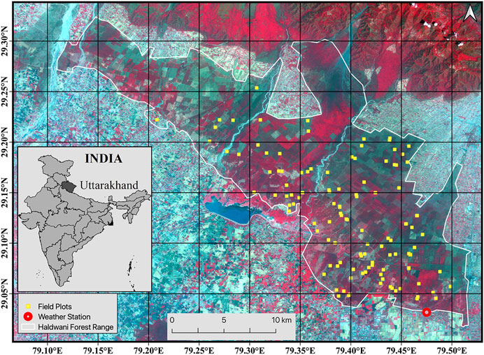
FIGURE 1. The Haldwani forest range as seen in a Sentinel-2 false color composite image acquired on May 12, 2018. Locations of the field plots and weather station are also shown.

The field campaign was carried out to collect parameters such as tree dbh (diameter at breast height or 1.3 m above ground), species, and tree height. A total of 93 field plots measuring 31.6 m × 31.6 m (0.1 ha) have been surveyed in November 2015 (N = 36), March 2017 (N = 13), and October-November 2018 (N = 44). The plots were generally established in homogeneous forest regions in either the uni-species compartments or mixed plantation compartments. We aimed to establish plots such that all the species and tree-age groups in the uni-species and mixed compartments are represented. However, certain compartments were not surveyed due to inaccessible forests or presence of wildlife. For each square field plot, the geolocation was tagged using a dual-frequency hand-held GPS receiver. The GPS receiver had a horizontal PDOP (position dilution of precision) between 5 m and 8 m and vertical PDOP between 1 m and 2 m. The tree height was measured using a combination of TruPulse 200 L rangefinder (±0.5 m range accuracy) and an LTI Criterion RD1000 distometer (1% height accuracy). Using the site- and species-specific volumetric equations given by the Forest Survey of India (1996), the volume of each tree was computed. Next, the tree and plot biomass is calculated using the species-specific wood density information available from the State Forest Department. The field measured AGB varies from 3.76 Mg/ha to 310 Mg/ha with a mean of 123 Mg/ha. Table 1 provides a summary of the minimum, maximum, arithmetic mean, and standard deviation of the parameters collected during the field campaigns.

TABLE 1

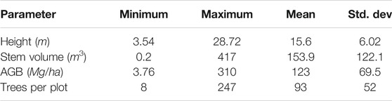
TABLE 1. Summary statistics of the various parameters collected during the field campaigns (Std. dev represents standard deviation).

The yield data available with the Uttarakhand State Forest Department showed that the average growth for a relatively mature forest compartment (age more than 15 years) was between 1 Mg/ha to 5 Mg/ha depending on the species and other factors (spacing between trees, soil and moisture conditions, etc.). However, the growth in AGB for new plantations is much higher, and reliable yield data is not available. As part of our field campaigns, three compartments were surveyed twice: once in 2015 and in 2018. These plots are in the same compartment, but not colocated as these are not permanent plots. The three compartments have relatively mature forests of Gutel, Teak, and Eucalyptus. Across those 3 years, the AGB increased by around 3–5 Mg/ha. Due to the relatively low growth in AGB, we assume a constant AGB over the time series for the relatively mature forests. For the plots in younger plantations, the AGB would increase across the time series. We have not considered these plots in this study and this is discussed further in Section 2.2.

The 4,390 trees surveyed in these plots are grouped into deciduous species (65%), evergreen species (20%), and mixed forests (15%). The 2013 National Forest Cover Map (FCM) generated by the Forest Survey of India classifies the forests broadly into four classes depending on canopy density. The Haldwani forest test site has 49% moderately dense forest (>70% canopy cover), 26% low-density forest (40–70% canopy cover), 23% open forest (10–40% canopy cover), and 2% nonforest regions.

Figure 2 shows the study area as imaged by the ALOS-2 data. The various forest compartments are clearly identified in this forest range due to silviculture practices. The GEDI observations over the study area are shown by the white dots. The field photographs show the different species and forest conditions across the test site. The weather station shown in Figure 1 and Figure 2 is located at the Pantnagar airport on the southern border of the Haldwani forest range. This weather station measures the temperature, precipitation, and wind speed at 3 h intervals. Figure 3 plots the precipitation on each day through the ALOS-2 acquisition timeline and the mean cross-polarized (HV) backscatter over the forest. The Indian monsoon season is clearly identified in this plot.

FIGURE 2

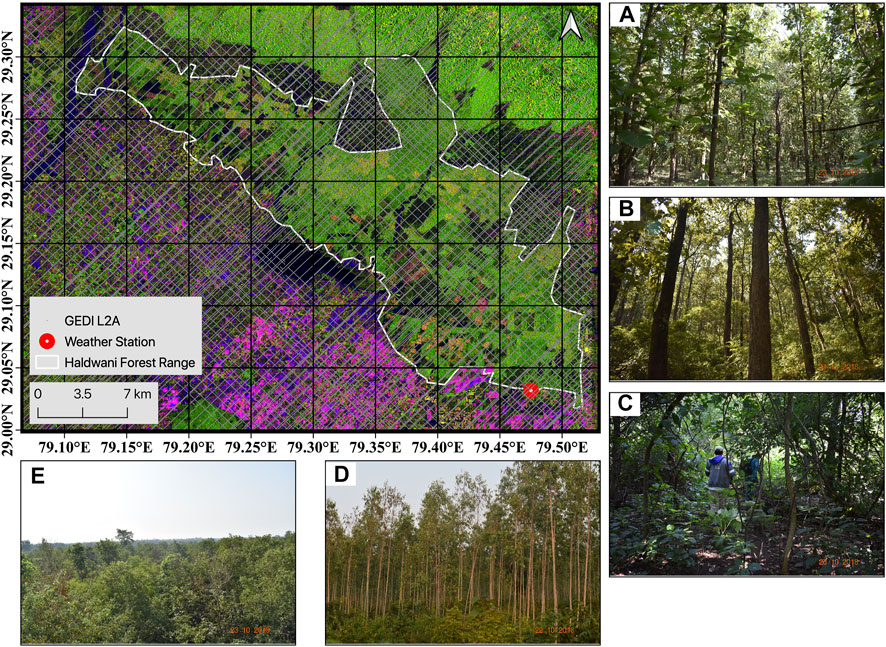
FIGURE 2. Haldwani forest range imaged by ALOS-2/PALSAR-2 (R:G:B = HH; HV; HH/HV). The location of the GEDI Level 2A observations over the test site is illustrated by the dense gray dots. The field photographs show (A) teak plantation, (B) high-AGB teak-dominated forest, (C) mixed forest, (D) Eucalyptus plantation, and (E) top of the canopy of the forest at a height of 25 m. All the field photographs are from the field campaign in October-November 2018.

FIGURE 3

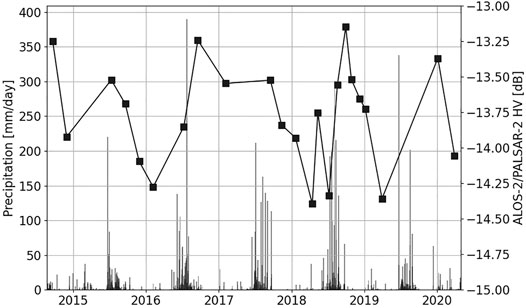
FIGURE 3. The daily precipitation is plotted over the acquisition timeline. Also shown in the mean cross-polarized (HV) backscatter of the 23 ALOS-2/PALSAR-2 acquisitions over the field plots shown in Figure 1.

2.2 ALOS-2/PALSAR-2 SAR Data

A time series of 23 dual-polarized (HH, HV), ascending pass, L-band ALOS-2 SAR data sets are acquired over the forest range. The time-series SAR data are acquired between September 2014 and March 2020. Table 2 shows the months of acquisition of the ALOS-2 data sets. The data are acquired in fine resolution dual-polarized strip-map mode and are provided in the SLC (single look complex) format. The incidence angle varies between 28.5° and 34.2°. The data are provided with azimuth spacing of 3.4 m and ground range spacing of 8.23 m. Here, we examine the cross-polarized (HV) channel relevant for forest biomass estimation using L-band SAR data.

TABLE 2

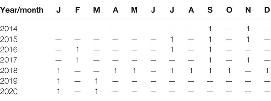
TABLE 2. Summary of available ALOS-2/PALSAR-2 dual-polarized (HH/HV) ascending pass acquisitions over Haldwani forest test site. There are 23 acquisitions spanning from September 2014 till March 2020.

Over the 5-year ALOS-2 time series, the forest compartments in the managed forests of the Haldwani range had clear-cuts as well as new plantations. The Uttarakhand State Forest Department provides a detailed report of the forest management practices in these compartments. Figure 4 shows examples of HV-polarization backscatter time series plotted for stable forest plots (Figures 4A,B), harvested forest plots (Figures 4C,D), and forests with growth (Figures 4E,F). The date of the field campaign for each plot are shown by a red dotted line and the AGB measured during the field campaign is also provided. The backscatter for plots in mature forest compartments has variations due to moisture and phenology changes, represented by the plots in Figures 4A,B. Plots in forest compartments which were clear-cut are shown in Figures 4C,D. For plot in Figure 4C, the compartment was replanted resulting in an increase in HV backscatter after harvest. Both growth plots (Figures 4E,F) exhibit an increase in HV backscatter up to 10 dB between 2015 and 2019. A total of 16 plots were excluded from this study which had new plantations or clear-cut of the forest. The remaining 77 plots are used to train and validate the forest AGB model.

FIGURE 4

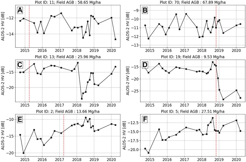
FIGURE 4. HV-pol backscatter time series of field plots representing stable forests (A) and (B); clear-cut forests (C) and (D); and growth in forests (E) and (F). The red dashed line represents the date of field campaign for each plot. The plot ID and the AGB measured during the field campaign are annotated.

2.3 GEDI Data

The GEDI Level 2A Elevation and Height Metrics data are available from the NASA/USGS Land Processes Distributed Active Archive Center (Dubayah et al., 2020b). The data over Haldwani was collected between April 2019 and April 2020. The data represents height return metrics for each of the 25 m diameter GEDI footprints. Figure 2 shows the GEDI footprints over the Haldwani forest range. The geolocated footprint data have 1-sigma positional errors of 10.3 m (Dubaya, 2021). For each footprint, we extracted height metrics from RH50 to RH100 corresponding to 50th to 100th percentile of energy return height relative to the ground. Each GEDI observation has six different versions of individual RH metric corresponding to the algorithm used (Potapov et al., 2021). We calculate the central mean (excluding minimum and maximum values) to obtain the RH metric value for each footprint.

2.4 Filtering GEDI Calibration Data

There are 32,710 GEDI observations covering the forest range delineated by the white border in Figure 2. To select the highest quality GEDI training and validation data, we use a filtering strategy which Potapov et al. (2021) applied to generate a global GEDI-derived forest height map. Only the power beams were selected, with observations collected during the night (to limit background noise), with beam sensitivity ≥ 0.9 and where the range of predicted ground elevation among the six algorithms was less than 2 m. The filtering resulted in 2200 GEDI samples.

2.5 Relating GEDI Height to Field Measured AGB

Many studies compare the GEDI percentile heights with a reference small footprint ALS-based heights to select the best GEDI metric for training models (e.g., see (Qi et al., 2019; Potapov et al., 2021)). However, in our case, airborne LiDAR data are not available over the study area. To calibrate GEDI height metrics, we collate the GEDI height with field measured plot height from the 0.1 ha field plots. As GEDI is a sampling mission, GEDI observations and the field plots are not always colocated. Among the 93 field plots, 32 field plots had overlapping GEDI observations. Three field plots were not considered as the forest had been harvested in the intervening years between the field campaign and GEDI observations. The remaining 29 field plots were all surveyed in 2015 and 2017, with no GEDI shots colocated with the field plots from the 2018 field campaign.

The field measured forest height was compared with RH metrics from RH50 to RH100. Figures 5A–C show the relation of the RH90, RH95, and RH100 height metrics with field height. The RH95 height metric performed the best with a correlation coefficient, R² of 0.67, and a root mean square error (RMSE) of 4.8 m. The RH95 height metric is related to field AGB using a power-law function as shown in Figure 5D. The GEDI AGB thus generated has an RMSE of 32 Mg/ha. This generates 2200 AGB sample points from GEDI to train and validate the forest AGB retrieval model. However, with the limited training samples used in relating GEDI height to field AGB, we use this data cautiously with the aim of getting a preliminary assessment of the advantages of combining L-band SAR and GEDI height metrics for improved forest AGB estimates.

FIGURE 5

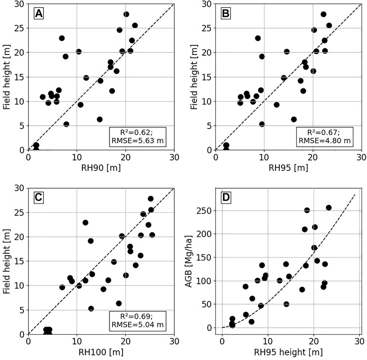
FIGURE 5. The GEDI RH heights correlated with field-measured height for the plots with overlapping GEDI observations. The RH95 height (B) shows the best performance. The RH95 height is further related to field measured AGB with a power-law relation to generate a GEDI-field AGB allometry.

3 Methodology

This section details the SAR and GEDI data processing workflows, the WCM model calibration process, and strategies used for forest AGB generation using the time-series SAR data. Figure 6 shows the overall methodological flow diagram, with the subsections detailing each step in further detail.

FIGURE 6

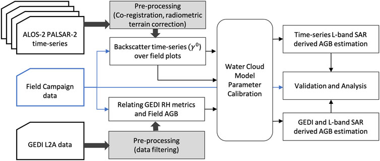
FIGURE 6. The flow diagram showing the overall methodology followed in this study.

3.1 ALOS-2/PALSAR-2 Data Processing

The ALOS-2/PALSAR-2 data acquired are in fine resolution dual-polarized strip-map SLC format. The data are radiometrically calibrated (Shimada et al., 2009) and coregistered using the orbit parameters and the 1-arc second NASADEM. Dense offsets are estimated and the SLCs are resampled to a reference acquisition, ensuring coregistration at the subpixel level. The ALOS-2 data are stored as radar backscatter σ⁰ (referenced to the flat ellipsoid), which is modulated by topography. An improved radiometric terrain correction (RTC) algorithm (Shiroma et al., 2020) is applied to flatten the backscatter and generate γ⁰. Our approach for RTC includes compensation of backscatter variation due to changing radar look angle across the imaged swath. The algorithm generates a flattened backscatter image ideally free of radiometric modulations caused by topography and incidence angle variations. In the RTC process, the field plot corners are projected to radar geometry, and subpixel aggregation of backscatter is carried out. Further, this aggregation approach ensures that there is no mismatch between pixel size and plot size, as even partially covered pixels are weighted according to their areal coverage. The number of spatial looks for calculating the average backscatter within the field plots is 42 ± 3 with minimum and maximum values of 34 and 53, respectively

3.2 Relating SAR Backscatter to AGB

The L-band backscatter is related to forest AGB using the three-parameter water cloud model (WCM) (Attema and Ulaby, 1978). The WCM model describes the forest as a volume of randomly oriented scatterers over an impermeable ground layer. At L-band, the modified version of WCM is used which accounts for vertical and horizontal discontinuities or gaps in the forest (Askne et al., 1997; Santoro et al., 2002). The WCM model has been used to relate L-band SAR backscatter to forest AGB in a number of studies (Santoro et al., 2011; Cartus et al., 2012; Kumar et al., 2012; Thiel and Schmullius, 2016; Khati et al., 2020) due to its strong physical foundations (Attema and Ulaby, 1978; Askne et al., 1997; Santoro et al., 2002) and computational simplicity.

The WCM model can be mathematically described as

${\gamma }^0=a{e}^{-c\beta }+b\left(1-e^{-c\beta }\right)(1)$

where the model parameters a, b, and c describe the scattering contribution from the ground through the canopy gaps, scattering contribution from the vegetation, and extinction of the wave through forest canopy, respectively. The term β is the AGB measured in Mg/ha. The derivation of Eq. (1) is not discussed here as it has been extensively discussed by Askne et al. (1997) and Santoro et al. (2002).

3.3 Model Training and Validation

The L-band cross-polarized (HV) backscatter measured over the seventy-seven 0.1 ha field plots is used for training and validation of the WCM model. For each of the 23 ALOS-2 acquisitions, the model parameters a, b, and c are estimated using the HV-pol backscatter and the field-derived AGB after applying a χ-squared minimization approach. The field plots are split randomly into 60% training and 40% test samples. The WCM model is calibrated using the training plots and validated on the test plots. The calibration and validation are iterated 30 times to capture the uncertainties and allow robust estimation of error. This generates the estimated AGB for each acquisition (B_i). It should be noted that we use all the 77 field plots across the ALOS-2 acquisitions spanning 5 years. For each acquisition, the performance of the WCM model derived AGB is assessed using the RMSE, coefficient of determination (R²), and the backscatter saturation level (β_sat). The RMSE and R² are calculated between the field measured AGB and WCM derived AGB. The backscatter saturation level for a given WCM model is defined as the value of biomass for which the biomass estimation error due to speckle equals the required modeled biomass estimation accuracy (Hensley et al., 2014). For our case, we considered the desired WCM model estimation accuracy of 20 Mg/ha in accordance with NISAR requirements. Solving the WCM models characterized by parameters a, b, and c for β = β_sat, we obtain the backscatter (γ_sat) at which the WCM curve saturates.

3.4 Time-Series AGB Estimation

The process detailed in Section 3.3 is applied to each of the 23 ALOS-2 acquisitions to obtain individual AGB estimates (B_i). These acquisitions asynchronously span 5 years (seen in Table 2) leading to uneven annual and seasonal coverage. The AGB estimates obtained from individual acquisitions can be impacted by nonhomogeneous environmental conditions (precipitation, soil, and canopy moisture) (Harrell et al., 1997; Pulliainen et al., 1999; Rauste, 2005; Cartus et al., 2012; Khati et al., 2020) or even ionospheric scintillation (Shimada et al., 2008; Belcher and Cannon, 2014). In our case, we do not observe any ionospheric scintillation. To improve the AGB estimation accuracy, we average the individual AGB estimates (B_i) to generate a multitemporal averaged AGB (B_mt) adopting an approach similar to Santoro et al. (2011).

$B_{mt}=\frac{{\sum }_{i=1}^N{B}_i}{N}(2)$

We modify this approach to capture the uncertainties associated with multitemporal AGB estimates. To estimate multitemporal AGB retrieval accuracy using N acquisitions, the N acquisition dates are chosen at random and the process is iterated 100 times. For example, with N = 5, the selected acquisitions might be all within 1 year (year 2018 has eight acquisitions) or might span the entire 5-year time span. Here, N ranges from 1 (single acquisition) to 23 (all acquisitions). For each N, the multitemporal AGB obtained is characterized by RMSE error and its standard deviation.

3.5 Relating GEDI Data to AGB

The GEDI height metrics are converted to AGB using the process detailed in Section 2.5. This results in 2,200 samples of AGB derived from GEDI height-field AGB allometry. The ALOS-2 backscatter for each of these GEDI shots is calculated. To reduce the noise within the data, we binned the GEDI data at 1 Mg/ha AGB intervals resulting in 227 samples. Larger binning intervals resulted in very few samples for low-AGB regions. For example, at 5 Mg/ha bins, there are only 49 samples of which 20 samples have AGB under 100 Mg/ha. The binned GEDI data are iteratively and randomly split into training and testing samples for calibration and validation of the WCM model. The GEDI-derived AGB is applied to train and validate the WCM model over each of the 23 ALOS-2 acquisitions. Further, multitemporal averaging as explained in the preceding section is applied to the estimated AGB. The accuracy of the modeled AGB using GEDI data is quantified using root mean square deviation (RMSD) measured with respect to the GEDI estimated AGB. Note that RMSD is used here as the parameter used to train the models (GEDI AGB) has an RMSE of 32 Mg/ha with respect to field measured AGB.

3.6 AGB Mapping and Comparison With Available Tropical AGB Products

Using the multitemporal ALOS-2 acquisitions, we derived the WCM model parameters using individual (B_i) and multitemporal (B_mt) AGB retrieval strategies. These parameters were used to invert the AGB and generate AGB maps of the Haldwani forest range and the surrounding regions. We use the TanDEM-X 50-m forest/nonforest (FNF) mask (Martone et al., 2018a,b) to mask out any nonforest regions. The mask is resampled to 25 m resolution using the nearest neighbor resampling method. Although this FNF data masks out some forest regions, it performs better than the ALOS-2 FNF over this test site. Using the mean of the AGB map generated for each ALOS-2 acquisition, the multitemporal mean AGB map is generated. We refer to this AGB map as ALOS-2 SLC AGB map.

To further assess the robustness of time-series ALOS-2 data for AGB mapping, we apply the WCM parameters on the globally available 25 m ALOS-2 yearly backscatter mosaics. The annual mosaic backscatter is available from 2015 till 2020. For each of these years, we calculated the WCM parameters from the multitemporal ALOS-2 acquisitions for those years. Inverting these parameters on the ALOS-2 global annual mosaics, we obtain the AGB maps over Haldwani. We used the TanDEM-X FNF to mask out the nonforest regions in this AGB map. We refer to this AGB map as the ALOS-2 annual mosaic generated AGB map.

We compare the generated AGB maps with available reference AGB products over the test site. The 2010 Global Biomass (GlobBiomass) (Santoro, 2018) map generated at 25 m resolution and the 1 km resolution pan-tropical biomass map (Avitabile et al., 2016) are used as reference AGB maps to qualitatively compare the generated AGB maps produced in this study. The RMSE between the field measured AGB and estimated AGB from these four maps is used for quantitative analysis.

4 Results and Discussion

4.1 Temporal Variation of Backscatter

The variation of backscatter as a function of field measured AGB is shown in Figure 7. Here, the mean ALOS-2 backscatter for each year is shown by the dots, and the standard deviation is shown by the error bars. The standard deviation of backscatter over the plots within a year is affected by the changes in weather (change in dielectric constant (Khati et al., 2020)), surface roughness (Wang et al., 1987; Ulaby et al., 1996; de Roo et al., 2001; Joseph et al., 2010), seasonal variations (leaf-on, leaf-fall (Khati et al., 2017; Bouvet et al., 2018)), and the number of annual acquisitions. The dotted line in each plot is the WCM curve estimated after calibrating the WCM model with the training samples. Here, the mean model parameters for each year’s acquisitions are used to plot the WCM curves.

FIGURE 7

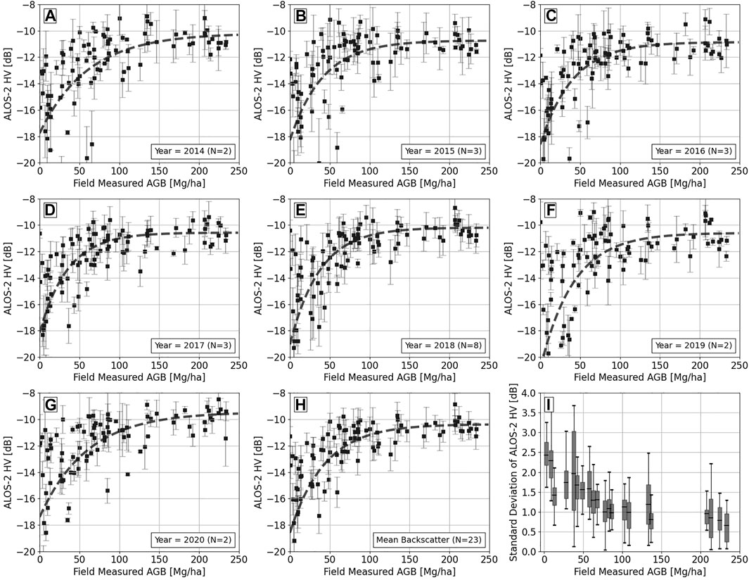
FIGURE 7. Mean annual ALOS-2 HV backscatter from 2014 to 2020 (A–G) plotted as a function of forest AGB with the WCM model curve. The whisker plots are the standard deviation of the backscatter. N shows the number of acquisitions available for each year over the site. The plot (H) shows the mean backscatter across all acquisitions plotted as a function of forest AGB. (I) is the HV backscatter multi-temporal standard deviation calculated for all acquisitions over the period 2014-2020.

Figure 7I shows the box plots of the temporal standard deviation (mean, quantiles, minimum, and maximum backscatter standard deviations) of ALOS-2 backscatter time series for different AGB ranges. Here, the AGB is grouped at every 5 Mg/ha range. This represents the temporal behavior of SAR backscatter as a function of the AGB level. Usually shorter trees (or low-biomass forests) have a larger temporal variability as the L-band SAR signal has higher penetration through the canopy and is influenced to a larger extent by the soil and canopy moisture variations, under-canopy structure changes, and degradation. The temporal standard deviation of backscatter decreases from a mean deviation of 2.5 dB for low-AGB regions (≥100 Mg/ha) to less than 1 dB for forests with AGB ≥ 100 Mg/ha. This shows that, for our case, we expect to have higher variations in backscatter over the time series for low-AGB regions. This is also seen in Figure 7H where the error bars show higher backscatter deviation for AGB ≤ 100 Mg/ha.

4.2 WCM Parameters

The iterative model training and validation approach explained in Section 3.3 was applied to all the 23 ALOS-2 acquisitions using a χ-squared minimization approach. The WCM model parameters a, b, and c and their standard deviation for each acquisition are estimated. We analyzed the impact of soil moisture, precipitation, and wind speed on the estimated WCM model parameters. In the absence of in situ soil moisture sensor data, the soil water index (SWI) derived from the Metop ASCAT sensor is used in this study. Although the resolution of this product is 0.1°, we observed a positive correlation with WCM parameter a (see Figure 8A). This is consistent with observations reported at L-band (Bouvet et al., 2018; Khati et al., 2020). Parameters b and c did not have any correlation with SWI as shown in Figure 8B and Figure 8C.

FIGURE 8

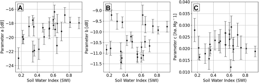
FIGURE 8. The estimated WCM model parameters (A–C) plotted against the soil water index (SWI) derived from the Metop ASCAT sensor. The parameter a shows a positive correlation with SWI while no such trend is observed for parameters (B,C).

The parameter a describes the scattering contribution from the ground and is more sensitive to changes in soil moisture, explaining its positive correlation with SWI. Parameter b describes the contribution of canopy components in the forest. Contrary to our findings in Lenor Landing, AL (Khati et al., 2020), we do not observe a positive correlation of parameter b with soil moisture. This can be attributed to the use of satellite-derived SWI product instead of in situ volumetric soil moisture measurements as used in (Khati et al., 2020). The SWI products are generated at coarser resolutions and typically represent the soil moisture content excluding the contributions from vegetation. Parameter c, representing the attenuation of the L-band SAR signal through the forest canopy, varies between 0.015 ha.Mg⁻¹ to 0.030 ha.Mg⁻¹. This is consistent with values reported by Bouvet et al. (2018) over Africa using ALOS/PALSAR data (between 0.0129 and 0.0291 ha.Mg⁻¹ for HV-pol). The parameter c varies with forest type as it is a function of vegetation water content and vegetation structure (Bouvet et al., 2018).

4.3 AGB Retrieval Performance

The retrieved WCM model parameters are used to estimate the forest AGB for each acquisition. The training and validation samples are iterated to obtain an estimate of the RMSE between the field measured AGB and WCM model estimated AGB. This is shown by the dotted line in Figure 9A. Additionally, the RMSE is also calculated for field plots with AGB less than 100 Mg/ha (according to the NISAR requirements) as shown by the solid line in Figure 9A. The overall RMSE varies between 58 Mg/ha and 73 Mg/ha for the 23 individual acquisitions. The RMSE for low-AGB forests varies between 32 Mg/ha and 69 Mg/ha. The saturation of the WCM curves (β = β_sat) for the 23 acquisitions varies between 65 Mg/ha and 125 Mg/ha with a mean of 96 Mg/ha. We observed that the saturation was higher for acquisitions with drier conditions (SWI ≤ 0.4) and decreased as SWI increased. However, the correlation was not significant.

FIGURE 9

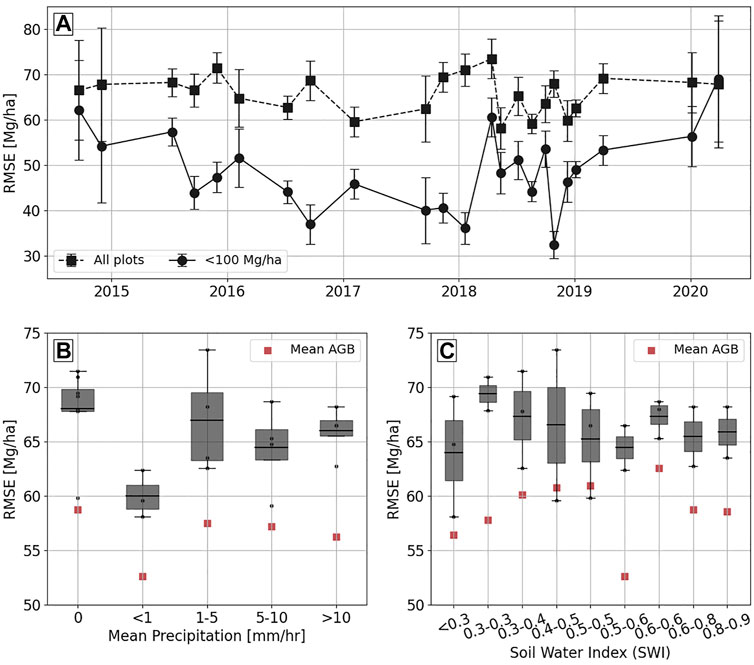
FIGURE 9. (A) The root mean squared error (RMSE) of the estimated AGB with respect to the field AGB for each ALOS-2/PALSAR-2 acquisition measured for all field plots and for plots with AGB less than 100 Mg/ha. (B,C) assess the impact of mean precipitation (72 h before acquisition) and SWI on model estimated AGB error.

The accuracy of AGB estimated from each acquisition depends on a number of factors including weather, soil and canopy moisture, changes in forest (disturbance and degradation), and model-fitting errors. Using the calibration and validation approach detailed in Section 3.3, we minimize the model-fitting errors. The field data is carefully selected removing any plots affected by forest changes (logging and growth). The impact of weather and moisture changes is analyzed in this study using the precipitation measured at the weather station and SWI estimated over the study area. The mean precipitation 72 h before the acquisition is used here. The box plots in Figure 9B and Figure 9C show the effect of precipitation and soil moisture on AGB estimation accuracy. The black dots show the RMSE for individual acquisition in each range of precipitation or SWI. There is an interesting trend between the RMSE of retrieved AGB and mean precipitation. For acquisitions in dry conditions (N = 8) the RMSE varies between 58 Mg/ha and 71 Mg/ha. Here, the RMSE is not influenced by precipitation but would be affected by other factors discussed earlier. Excluding the acquisitions in dry conditions, the RMSE increases with precipitation. The mean RMSE is 60 Mg/ha for light precipitation (≤1 mm/h) acquisitions and increases to 66 Mg/ha for acquisitions with higher precipitations. For acquisitions with low soil moisture (SWI ≤ 0.3), we observe RMSE between 58 Mg/ha and 68 Mg/ha. Here, we are considering acquisitions with SWI values between selected intervals. For acquisitions with higher SWI, the RMSE is slightly higher between 65 Mg/ha and 70 Mg/ha.

The red squares in Figure 9B and Figure 9C represent the RMSE of mean AGB for acquisitions within each precipitation and SWI interval. For example, there are eight acquisitions with zero precipitation. The mean AGB from these eight acquisitions is used to estimate the RMSE shown by the red square in Figure 9D. It is interesting to note that the impact of precipitation up to 10 mm/h can be minimized using mean AGB estimates as seen by the red squares in Figure 9B.

4.4 Multitemporal AGB Retrieval

To take advantage of the multitemporal acquisitions and assess their use in improving the AGB estimates, we use the mean of the AGB estimates from each individual acquisition. Adding more acquisitions improves the AGB estimates. We randomly selected any N acquisitions with 1 ≤ N ≤ 23. Figure 10A shows that the RMSE decreases from 65 Mg/ha to 55 Mg/ha with an increase in the number of acquisitions used to estimate multitemporal AGB. Similarly, for low-AGB regions, the RMSE improves from 49 Mg/ha to 38 Mg/ha. Thus, using the multitemporal AGB retrieval approach, we observed an overall improvement in AGB estimation accuracy of 16% for all field plots and 21% for plots with AGB ≤ 100 Mg/ha (Figure 10B). Figure 10C shows the deviation of the error for the increasing number of acquisitions. The stability of AGB estimates improves with additional acquisitions. From this analysis, we can observe that 1) after ten acquisitions, the improvement in AGB estimation accuracy with each additional acquisition is not significant and 2) the variations in backscatter due to changes in soil and canopy conditions are better absorbed with the use of multitemporal acquisitions.

FIGURE 10

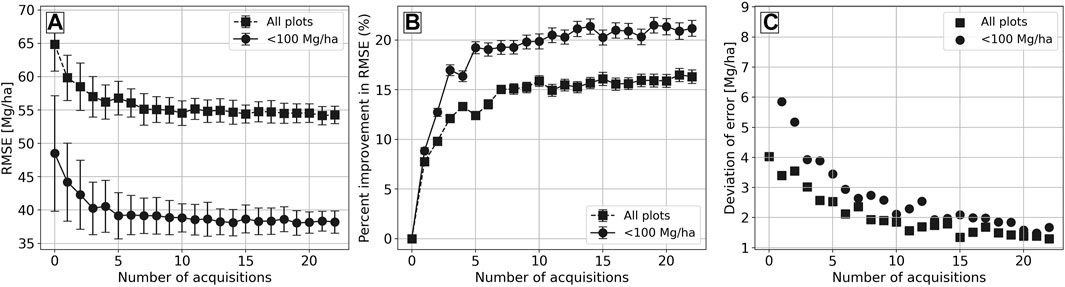
FIGURE 10. (A) shows the improvement in RMSE and (B) shows the percent improvement in RMSE (B) of the estimated AGB when time-series acquisitions are used. (C) describes the reduction in deviation of the measured error in AGB estimates with an increase in the number of acquisitions used.

This improvement in AGB estimation using multitemporal data is consistent with findings reported in the literature. Cartus et al. (2012) reported that, over the North-Eastern United States, using ten ALOS/PALSAR acquisitions, the overall RMSD improved by 23.6% from 55 Mg/ha for single acquisitions to 42 Mg/ha for multitemporal averaging. A similar analysis using multitemporal ALOS-2 SAR data over Mondah and Lope forest sites in Gabon is reported by Cartus and Santoro (2019). Their study assesses that, using multitemporal L-band SAR acquisitions, the %RMSE (percentage of mean AGB) improves from 135% to 89% for Mondah and from around 60% to 45–50% for Lope forest test sites. Using four ALOS-2 acquisitions over a Chinese fir-dominated forest, the AGB estimation accuracy improved from a %RMSE of 33.8% for a single acquisition to 24.4% when multitemporal data were used (Long et al., 2020). However, over a Pine and Eucalyptus-dominated semiarid forest in Australia, Tanase et al. (2014) report that the multitemporal approach provides more reliable AGB estimates but did not improve the AGB estimation accuracy significantly. Extensive analysis carried over Swedish forest sites using ALOS/PALSAR data shows that, using HV-pol backscatter, the RMSE improves by 50% or more when multitemporal retrieval strategies were used (Santoro et al., 2015).

4.5 GEDI- and ALOS-2-Based Forest AGB Retrieval

As described in Section 3.5, 227 binned samples of the GEDI AGB were used to calibrate the WCM models using the HV-pol backscatter of all 23 ALOS-2 acquisitions. The WCM model parameters were used to invert the forest AGB. The RMSD of the WCM-inverted AGB (with respect to the GEDI-derived AGB) for each acquisition is shown in Figure 11A. The RMSD ranges between 55 Mg/ha and 88 Mg/ha. The WCM curves for the GEDI samples saturates between 55 Mg/ha and 95 Mg/ha as shown in Figure 11B. The saturation of the WCM curves was lower for acquisitions after August 2018.

FIGURE 11

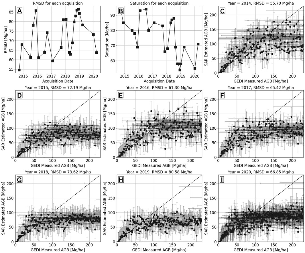
FIGURE 11. (A) shows the RMSE of the WCM estimated AGB with respect to the GEDI measured AGB, and (B) shows saturation of the WCM curve for each ALOS-2/PALSAR-2 acquisition. The scatter plots in (C–I) compare the multitemporal AGB estimates using ALOS-2 data acquired each year with the GEDI measured AGB. The error bars along the abscissa represent the RMSE in the GEDI measured AGB, while the error bars along the ordinate represent the standard deviation of the AGB estimates for each year.

To test the utility of combining multiple ALOS-2 acquisitions with GEDI, we use the multitemporal average of the estimated AGB. We observed that combining multiple AGB estimates did not lead to any significant improvement in AGB estimation accuracy. The RMSD reduced from 70 ± 8 Mg/ha (using single acquisition) to 66 ± 3 Mg/ha (using all 23 acquisitions). To analyze further, we used the acquisitions from each year to obtain the multitemporal AGB estimates. Figures 11C–I show the validation plots comparing the GEDI measured AGB with the SAR estimated AGB. The error bars along the abscissa represent the RMSE in the GEDI measured AGB, while the error bars along the ordinate represent the standard deviation of the AGB estimates for each year.

The multitemporal AGB estimated from 2014 and 2016 acquisitions performs better with RMSD of 55.7 Mg/ha and 61.3 Mg/ha, respectively. The multitemporal AGB estimates from 2018 and later show lower accuracy. This might be due to the bias in the plots used for GEDI AGB estimation. As discussed in Section 2.5, the plots used for training the GEDI height-field AGB models are all acquired in 2015 and 2017. Further, we have a limited number of colocated plots which are not representative of all the forest species or density classes in the test site. The changes in the forest after 2017 might not be completely characterized by the GEDI AGB, leading to higher uncertainties in the WCM modeled AGB estimates for acquisitions after 2017.

4.6 Comparison of AGB Maps With Available Data Sets

The AGB maps are generated using the ALOS-2 multitemporal acquisitions and the ALOS-2 annual global backscatter mosaic as described in Section 3.6. A subset of the generated AGB maps from ALOS-2 SLC and ALOS-2 annual mosaic are shown in Figures 12A,B, respectively. The AGB maps over the test site from the GlobBiomass and the pan-tropical biomass products are shown in Figures 12C,D, respectively. Note that maps in Figures 12A–C are at 25 m resolution, while the pan-tropical AGB map in Figure 12D is at 1 km resolution. The four AGB maps have a common color map which is clipped at 200 Mg/ha for easier comparison and visualization.

FIGURE 12

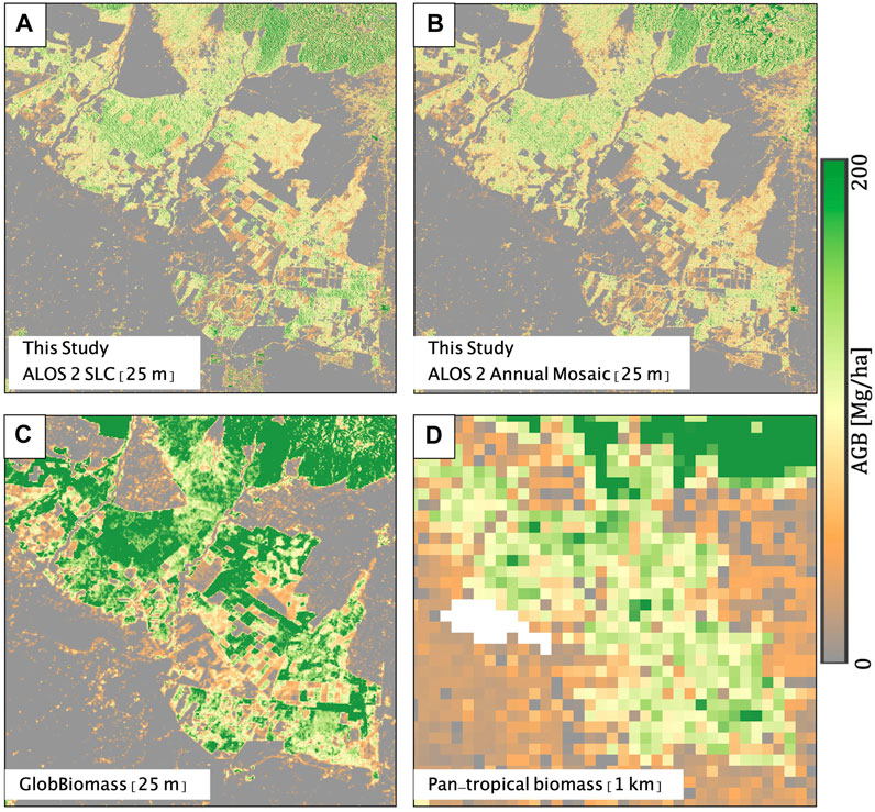
FIGURE 12. The AGB maps generated using the multitemporal mean AGB of (A) 23 ALOS-2/PALSAR-2 SLC acquisitions and (B) yearly ALOS-2/PALSAR-2 global mosaics. The generated AGB maps are compared with available AGB maps from (C) GlobBiomass (Santoro, 2018) and (D) pan-tropical AGB (Avitabile et al., 2016). The pan-tropical AGB is at 1 km resolution while the other maps are generated at 25 m resolution.

Figure 13 shows the validation scatter plots between the field measured AGB and the AGB estimated by the generated AGB maps (Figures 13A,B) and the reference AGB maps (Figures 13C,D). The RMSE and the number of field plots imaged are also shown. The number of field plots is lower for ALOS-2 SLC and ALOS-2 annual mosaic generated AGB maps due to the use of TanDEM-X FNF which masked a few forest areas. The RMSE for the AGB map generated in this study using the ALOS-2 time series is the lowest at 62 Mg/ha. The AGB generated using ALOS-2 annual mosaic has the highest RMSE. This might be due to higher uncertainties in the global mosaic backscatter. Also, the WCM model parameters trained on ALOS-2 SLC data applied to the backscatter mosaic adds additional errors. The GlobBiomass AGB product shows good retrieval accuracy despite the 5- to 7-year gap between the AGB map generation in 2010 and the field measurements. The saturation of the WCM model estimated AGB around 100 Mg/ha is clearly observed in Figure 13A. Although the GlobBiomass product has a higher AGB saturation level, its variance along the correlation line is also higher. The 1 km resolution pan-tropical biomass product does not show any correlation with field measured AGB due to the coarser resolution.

FIGURE 13

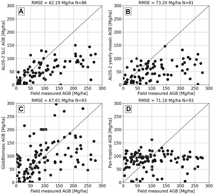
FIGURE 13. The validation scatter plots compare the field measured AGB with the multitemporal mean AGB of (A) 23 ALOS-2/PALSAR-2 SLC acquisitions, (B) yearly ALOS-2/PALSAR-2 global mosaics, (C) GlobBiomass (Santoro, 2018), and (D) pan-tropical AGB (Avitabile et al., 2016).

5 Conclusion

In this paper, we analyze the potential of multitemporal ALOS-2 acquisitions to improve AGB estimates over a subtropical forest using the 3-parameter WCM model and 0.1 ha field inventory plots. The novelty of this research work is that it aims to assess the improvement in AGB with L-band time-series data along with the impact of the higher uncertainties in field inventory data due to relatively small plot size. The small plot size combined with multiple field campaigns spread over 3 years might lead to higher errors in the field inventory data. As this is a managed forest with uni-species compartments, the possibility of these plots not capturing the variability in the forest is reduced significantly. However, due to the forest management practices, the forest compartments undergo changes (logging and plantation) which might impact WCM model calibration. The influence of such plots on the analysis carried out is reduced due to the change detection analysis carried out for the 93 plots as shown in Figure 4. Our analysis shows that forest AGB retrieval improves by aggregating multitemporal AGB estimates from L-band HV SAR backscatter time series. For single L-band acquisitions, the RMSE of the estimated AGB varies between 60 Mg/ha and 75 Mg/ha. With multitemporal averaging, the AGB estimation accuracy improves by up to 16% with RMSE decreasing to 55 Mg/ha. Note that this approach leads to retrieval accuracy better than any of the individual AGB estimates. Furthermore, this analysis shows that the AGB estimation accuracy improves by 21% for forests with AGB less than 100 Mg/ha. Using more than ten ALOS-2 acquisitions in the multitemporal AGB retrieval approach did not lead to significant improvement in AGB estimates for the managed forest under study.

The RMSE with multitemporal retrieval is around 44% of mean AGB and is relatively high. However, if we consider only the low-AGB forest regions (≤100 Mg/ha), then the retrieval accuracy with multitemporal data results in AGB products with RMSE of 39 Mg/ha (31% of mean AGB). These errors can be further reduced if 1) larger (>0.5 ha) and permanent field plots are available, 2) small footprint ALS data or NFI data are accessible, which would reduce the uncertainties in the field inventory data, and 3) denser L-band timeseries is acquired leading to a lower temporal gap between field inventory and acquisitions. This work assumes importance from the perspective of the NISAR mission’s goals to generate global forest AGB products. The NISAR mission would acquire up to 30 acquisitions per year over a target and generate global AGB products for forests with AGB up to 100 Mg/ha. The products would achieve an RMS error of 20 Mg/ha or better. Although the NISAR biomass products may be generated using more complex algorithms taking into account the seasonal and weather-induced changes in SAR backscatter, there is limited ground inventory data over most of the tropical and subtropical forests. Among the other findings, this work confirms that, using denser time-series L-band data and more complex algorithms, it would be possible to generate AGB products which would achieve the desired accuracy.

Further, this research work provides a preliminary analysis of the AGB products that can be generated using the GEDI height metrics and ALOS-2 time series. It should be noted that we have a limited set of colocated field plots that were used to relate GEDI height metrics with field AGB. The analysis presented shows the potential of improved AGB estimation using a fusion of GEDI height metrics and L-band SAR backscatter time series.

Data Availability Statement

The distribution of SAR and field raw data supporting the conclusion of this study is restricted because of project agreements between the authors and the data providers. Requests to access the processed data should be directed to the corresponding author.

Author Contributions

Conceptualization: UK and ML; methodology: UK and ML; data acquisition: GS; data curation, processing, and analysis: UK; infrastructure support: ML; fieldwork collection: UK; writing—original draft preparation: UK; writing—review and editing: ML and GS; supervision, ML; project administration, ML; funding acquisition, ML.

Funding

This work was conducted at the Jet Propulsion Laboratory, California Institute of Technology, under contract with NASA as part of the NISAR Project Science Team activities.

Conflict of Interest

The authors declare that the research was conducted in the absence of any commercial or financial relationships that could be construed as a potential conflict of interest.

Publisher’s Note

All claims expressed in this article are solely those of the authors and do not necessarily represent those of their affiliated organizations, or those of the publisher, the editors and the reviewers. Any product that may be evaluated in this article, or claim that may be made by its manufacturer, is not guaranteed or endorsed by the publisher.

Acknowledgments

The authors thank the NISAR Project and Algorithm Definition Team (ADT) for providing the InSAR Scientific Computing Environment (ISCE3) software that was used for coregistering and radiometric terrain correcting the ALOS-2/PALSAR-2 SLC stack. The authors would like to thank the Japanese Aerospace Exploration Agency (JAXA) for ALOS-2/PALSAR-2 data under Project No: JAXA-3055, the Global Ecosystem Dynamics Investigation (GEDI) team for acquiring the lidar data set, the German Aerospace Agency (DLR) for 12 m TanDEM-X DEM under science phase AO Project No. DEM_GLAC1805, and also the Uttarakhand State Forest Department for technical support during field campaigns.

References

Antropov, O., Rauste, Y., Ahola, H., and Hame, T. (2013). Stand-Level Stem Volume of Boreal Forests from Spaceborne SAR Imagery at L-Band. IEEE J. Sel. Top. Appl. Earth Obs. Remote Sensing 6, 35–44. doi:10.1109/JSTARS.2013.2241018

CrossRef Full Text | Google Scholar

Askne, J., Fransson, J., Santoro, M., Soja, M., and Ulander, L. (2013). Model-Based Biomass Estimation of a Hemi-Boreal Forest from Multitemporal TanDEM-X Acquisitions. Remote Sensing 5, 5574–5597. doi:10.3390/rs5115574

CrossRef Full Text | Google Scholar

Askne, J. I. H., Dammert, P. B. G., Ulander, L. M. H., and Smith, G. (1997). C-band Repeat-Pass Interferometric SAR Observations of the forest. IEEE Trans. Geosci. Remote Sensing 35, 25–35. doi:10.1109/36.551931

CrossRef Full Text | Google Scholar

Attema, E. P. W., and Ulaby, F. T. (1978). Vegetation Modeled as a Water Cloud. Radio Sci. 13, 357–364. doi:10.1029/RS013i002p00357

CrossRef Full Text | Google Scholar

Avitabile, V., Herold, M., Heuvelink, G. B. M., Lewis, S. L., Phillips, O. L., Asner, G. P., et al. (2016). An Integrated pan‐tropical Biomass Map Using Multiple Reference Datasets. Glob. Change Biol. 22, 1406–1420. doi:10.1111/gcb.13139

PubMed Abstract | CrossRef Full Text | Google Scholar

Belcher, D. P., and Cannon, P. S. (2014). Amplitude Scintillation Effects on Sar. IET Radar Sonar Navig. 8, 658–666. doi:10.1049/iet-rsn.2013.0168

CrossRef Full Text | Google Scholar

Bouvet, A., Mermoz, S., Le Toan, T., Villard, L., Mathieu, R., Naidoo, L., et al. (2018). An Above-Ground Biomass Map of African Savannahs and Woodlands at 25 M Resolution Derived from ALOS PALSAR. Remote Sensing Environ. 206, 156–173. doi:10.1016/j.rse.2017.12.030

CrossRef Full Text | Google Scholar

Burgin, M., Clewley, D., Lucas, R. M., and Moghaddam, M. (2011). A Generalized Radar Backscattering Model Based on Wave Theory for Multilayer Multispecies Vegetation. IEEE Trans. Geosci. Remote Sensing 49, 4832–4845. doi:10.1109/tgrs.2011.2172949

CrossRef Full Text | Google Scholar

Cartus, O., and Santoro, M. (2019). Exploring Combinations of Multi-Temporal and Multi-Frequency Radar Backscatter Observations to Estimate Above-Ground Biomass of Tropical forest. Remote Sensing Environ. 232, 111313. doi:10.1016/j.rse.2019.111313

CrossRef Full Text | Google Scholar

Cartus, O., Santoro, M., and Kellndorfer, J. (2012). Mapping forest Aboveground Biomass in the Northeastern United States with ALOS PALSAR Dual-Polarization L-Band. Remote Sensing Environ. 124, 466–478. doi:10.1016/j.rse.2012.05.029

CrossRef Full Text | Google Scholar

Chave, J., Condit, R., Aguilar, S., Hernandez, A., Lao, S., and Perez, R. (2004). Error Propagation and Scaling for Tropical forest Biomass Estimates. Phil. Trans. R. Soc. Lond. B 359, 409–420. doi:10.1098/rstb.2003.1425

PubMed Abstract | CrossRef Full Text | Google Scholar

de Roo, R. D., Yang Du, Du., Ulaby, F. T., and Dobson, M. C. (2001). A Semi-empirical Backscattering Model at L-Band and C-Band for a Soybean Canopy with Soil Moisture Inversion. IEEE Trans. Geosci. Remote Sensing 39, 864–872. doi:10.1109/36.917912

CrossRef Full Text | Google Scholar

Dobson, M. C., Ulaby, F. T., LeToan, T., Beaudoin, A., Kasischke, E. S., and Christensen, N. (1992). Dependence of Radar Backscatter on Coniferous forest Biomass. IEEE Trans. Geosci. Remote Sensing 30, 412–415. doi:10.1109/36.134090

CrossRef Full Text | Google Scholar

Dubaya, S. T. (2021). Global Ecosystem Dynamics Investigation (GEDI) Level 2 User Guide College Park, MD: University of Maryland.

Google Scholar

Dubayah, R., Blair, J. B., Goetz, S., Fatoyinbo, L., Hansen, M., and Healey, S. (2020a). The Global Ecosystem Dynamics Investigation: High-resolution laser ranging of the Earth’s forests and topography. Sci. Remote Sensing 1, 100002. doi:10.1016/j.srs.2020.100002

CrossRef Full Text | Google Scholar

Dubayah, R., Hofton, M., Blair, J., Armston, J., Tang, H., and Luthcke, S. (2020b). GEDI L2A Elevation and Height Metrics Data Global Footprint Level V002 [data Set] NASA EOSDIS Land Processes DAAC. Available at: https://lpdaac.usgs.gov/products/gedi02_av001/. Accessed June 16, 2021

Google Scholar

Englhart, S., Keuck, V., and Siegert, F. (2012). Modeling Aboveground Biomass in Tropical Forests Using Multi-Frequency SAR Data-A Comparison of Methods. IEEE J. Sel. Top. Appl. Earth Observations Remote Sensing 5, 298–306. doi:10.1109/JSTARS.2011.2176720

CrossRef Full Text | Google Scholar

Forest Survey of India (1996). Volume Equations for Forests of India, Nepal, and Bhutan. Dehradun: Forest Survey of India, Ministry of Environment & Forests, Government of India).

Google Scholar

Ghasemi, N., Sahebi, M. R., and Mohammadzadeh, A. (2011). A Review on Biomass Estimation Methods Using Synthetic Aperture Radar Data. Int. J. Geomat. Geosci. 1, 13.

Google Scholar

Hall, F. G., Bergen, K., Blair, J. B., Dubayah, R., Houghton, R., Hurtt, G., et al. (2011). Characterizing 3d Vegetation Structure from Space: Mission Requirements. Remote Sensing Environ. 115, 2753–2775. doi:10.1016/j.rse.2011.01.024

CrossRef Full Text | Google Scholar

Harrell, P. A., Kasischke, E. S., Bourgeau-Chavez, L. L., Haney, E. M., and Christensen, N. L. (1997). Evaluation of Approaches to Estimating Aboveground Biomass in Southern pine Forests Using SIR-C Data. Remote Sensing Environ. 59, 223–233. doi:10.1016/S0034-4257(96)00155-1

CrossRef Full Text | Google Scholar

Hensley, S., Oveisgharan, S., Saatchi, S., Simard, M., Ahmed, R., and Haddad, Z. (2014). An Error Model for Biomass Estimates Derived from Polarimetric Radar Backscatter. IEEE Trans. Geosci. Remote Sensing 52, 4065–4082. doi:10.1109/TGRS.2013.2279400

CrossRef Full Text | Google Scholar

Houghton, R. A., Lawrence, K. T., Hackler, J. L., and Brown, S. (2001). The Spatial Distribution of forest Biomass in the Brazilian Amazon: a Comparison of Estimates. Glob. Change Biol. 7, 731–746. doi:10.1046/j.1365-2486.2001.00426.x

CrossRef Full Text | Google Scholar

Huang, W., Sun, G., Ni, W., Zhang, Z., and Dubayah, R. (2015). Sensitivity of Multi-Source SAR Backscatter to Changes in Forest Aboveground Biomass. Remote Sensing 7, 9587–9609. doi:10.3390/rs70809587

CrossRef Full Text | Google Scholar

Hubbell, S. P., Foster, R. B., O’Brien, S. T., Harms, K. E., Condit, R., Wechsler, B., et al. (1999). Light-Gap Disturbances, Recruitment Limitation, and Tree Diversity in a Neotropical Forest. Science 283, 554–557. doi:10.1126/science.283.5401.554

PubMed Abstract | CrossRef Full Text | Google Scholar

Joseph, A. T., van der Velde, R., O'Neill, P. E., Lang, R., and Gish, T. (2010). Effects of Corn on C- and L-Band Radar Backscatter: A Correction Method for Soil Moisture Retrieval. Remote Sensing Environ. 114, 2417–2430. doi:10.1016/j.rse.2010.05.017

CrossRef Full Text | Google Scholar

Joshi, N., Mitchard, E. T. A., Brolly, M., Schumacher, J., Fernández-Landa, A., Johannsen, V. K., et al. (2017). Understanding 'saturation' of Radar Signals over Forests. Sci. Rep. 7, 3505. doi:10.1038/s41598-017-03469-3

PubMed Abstract | CrossRef Full Text | Google Scholar

Kasischke, E. S., Melack, J. M., and Craig Dobson, M. (1997). The Use of Imaging Radars for Ecological Applications-A Review. Remote Sensing Environ. 59, 141–156. doi:10.1016/S0034-4257(96)00148-4

CrossRef Full Text | Google Scholar

Khati, U., Lavalle, M., Shiroma, G. H. X., Meyer, V., and Chapman, B. (2020). Assessment of forest Biomass Estimation from Dry and Wet Sar Acquisitions Collected during the 2019 Uavsar Am-Pm Campaign in southeastern united states. Remote Sensing 12, 3397. doi:10.3390/rs12203397

CrossRef Full Text | Google Scholar

Khati, U., Lavalle, M., and Singh, G. (2019). Spaceborne Tomography of Multi-Species Indian Tropical Forests. Remote Sensing Environ. 229, 193–212. doi:10.1016/j.rse.2019.04.017

CrossRef Full Text | Google Scholar

Khati, U., Singh, G., and Ferro-Famil, L. (2017). Analysis of Seasonal Effects on forest Parameter Estimation of Indian Deciduous forest Using TerraSAR-X PolInSAR Acquisitions. Remote Sensing Environ. 199, 265–276. doi:10.1016/j.rse.2017.07.019

CrossRef Full Text | Google Scholar

Khati, U., Singh, G., and Kumar, S. (2018). Potential of Space-Borne PolInSAR for Forest Canopy Height Estimation over India-A Case Study Using Fully Polarimetric L-, C-, and X-Band SAR Data. IEEE J. Sel. Top. Appl. Earth Obs. Remote Sensing 11, 2406–2416. doi:10.1109/jstars.2018.2835388

CrossRef Full Text | Google Scholar

Kumar, S., Pandey, U., Kushwaha, S. P., Chatterjee, R. S., and Bijker, W. (2012). Aboveground Biomass Estimation of Tropical forest from Envisat Advanced Synthetic Aperture Radar Data Using Modeling Approach. J. Appl. Remote Sens. 6, 063588. doi:10.1117/1.JRS.6.063588

CrossRef Full Text | Google Scholar

Kurvonen, L., Pulliainen, J., and Hallikainen, M. (1999). Retrieval of Biomass in Boreal Forests from Multitemporal ERS-1 and JERS-1 SAR Images. IEEE Trans. Geosci. Remote Sensing 37, 198–205. doi:10.1109/36.739154

CrossRef Full Text | Google Scholar

Le Toan, T., Beaudoin, A., Riom, J., and Guyon, D. (1992). Relating forest Biomass to SAR Data. IEEE Trans. Geosci. Remote Sensing 30, 403–411. doi:10.1109/36.134089

CrossRef Full Text | Google Scholar

Le Toan, T., Quegan, S., Davidson, M. W. J., Balzter, H., Paillou, P., Papathanassiou, K., et al. (2011). The BIOMASS mission: Mapping Global forest Biomass to Better Understand the Terrestrial Carbon Cycle. Remote Sensing Environ. 115, 2850–2860. doi:10.1016/j.rse.2011.03.020

CrossRef Full Text | Google Scholar

Long, J., Lin, H., Wang, G., Sun, H., and Yan, E. (2020). Estimating the Growing Stem Volume of the Planted Forest Using the General Linear Model and Time Series Quad-Polarimetric SAR Images. Sensors 20, 3957. doi:10.3390/s20143957

PubMed Abstract | CrossRef Full Text | Google Scholar

Lucas, R., Armston, J., Fairfax, R., Fensham, R., Accad, A., Carreiras, J., et al. (2010). An Evaluation of the ALOS PALSAR L-Band Backscatter-Above Ground Biomass Relationship Queensland, Australia: Impacts of Surface Moisture Condition and Vegetation Structure. IEEE J. Sel. Top. Appl. Earth Obs. Remote Sensing 3, 576–593. doi:10.1109/JSTARS.2010.2086436

CrossRef Full Text | Google Scholar

Lucas, R. M., Cronin, N., Lee, A., Moghaddam, M., Witte, C., and Tickle, P. (2006). Empirical Relationships between AIRSAR Backscatter and LiDAR-Derived forest Biomass, Queensland, Australia. Remote Sensing Environ. 100, 407–425. doi:10.1016/j.rse.2005.10.019

CrossRef Full Text | Google Scholar

Lucas, R. M., Moghaddam, M., and Cronin, N. (2004). Microwave Scattering from Mixed-Species Forests, Queensland, Australia. IEEE Trans. Geosci. Remote Sensing 42, 2142–2159. doi:10.1109/TGRS.2004.834633

CrossRef Full Text | Google Scholar

Luckman, A., Baker, J., Honzák, M., and Lucas, R. (1998). Tropical Forest Biomass Density Estimation Using JERS-1 SAR: Seasonal Variation, Confidence Limits, and Application to Image Mosaics. Remote Sensing Environ. 63, 126–139. doi:10.1016/S0034-4257(97)00133-8

CrossRef Full Text | Google Scholar

Luckman, A., Baker, J., Kuplich, T. M., Yanasse, C. d. C. F., and Frery, A. (1997). A Study of the Relationship between Radar Backscatter and Regenerating Tropical forest Biomass for Spaceborne SAR Instruments. Remote Sensing Environ. 60, 1–13. doi:10.1016/s0034-4257(96)00121-6

CrossRef Full Text | Google Scholar

Martone, M., Rizzoli, P., Wecklich, C., González, C., Bueso-Bello, J.-L., Valdo, P., et al. (2018a). The Global forest/non-forest Map from Tandem-X Interferometric Sar Data. Remote Sensing Environ. 205, 352–373. doi:10.1016/j.rse.2017.12.002

CrossRef Full Text | Google Scholar

Martone, M., Sica, F., González, C., Bueso-Bello, J.-L., Valdo, P., and Rizzoli, P. (2018b). High-resolution forest Mapping from Tandem-X Interferometric Data Exploiting Nonlocal Filtering. Remote Sensing 10, 1477. doi:10.3390/rs10091477

CrossRef Full Text | Google Scholar

Musthafa, M., Khati, U., and Singh, G. (2020). Sensitivity of Polsar Decomposition to forest Disturbance and Regrowth Dynamics in a Managed forest. Adv. Space Res. 66, 1863–1875. doi:10.1016/j.asr.2020.07.007

CrossRef Full Text | Google Scholar

Ningthoujam, R., Balzter, H., Tansey, K., Morrison, K., Johnson, S., Gerard, F., et al. (2016). Airborne S-Band SAR for Forest Biophysical Retrieval in Temperate Mixed Forests of the UK. Remote Sensing 8, 609. doi:10.3390/rs8070609

CrossRef Full Text | Google Scholar

Ningthoujam, R. K., Joshi, P. K., and Roy, P. S. (2018). Retrieval of forest Biomass for Tropical Deciduous Mixed forest Using ALOS PALSAR Mosaic Imagery and Field Plot Data. Int. J. Appl. Earth Obs. Geoinf. 69, 206–216. doi:10.1016/j.jag.2018.03.007

CrossRef Full Text | Google Scholar

Peregon, A., and Yamagata, Y. (2013). The Use of ALOS/PALSAR Backscatter to Estimate Above-Ground forest Biomass: A Case Study in Western Siberia. Remote Sensing Environ. 137, 139–146. doi:10.1016/j.rse.2013.06.012

CrossRef Full Text | Google Scholar

Potapov, P., Li, X., Hernandez-Serna, A., Tyukavina, A., Hansen, M. C., Kommareddy, A., et al. (2021). Mapping Global forest Canopy Height through Integration of GEDI and Landsat Data. Remote Sensing Environ. 253, 112165. doi:10.1016/j.rse.2020.112165

CrossRef Full Text | Google Scholar

Pulliainen, J. T., Kurvonen, L., and Hallikainen, M. T. (1999). Multitemporal Behavior of L- and C-Band Sar Observations of Boreal Forests. IEEE Trans. Geosci. Remote Sensing 37, 927–937. doi:10.1109/36.752211

CrossRef Full Text | Google Scholar

Qi, W., Saarela, S., Armston, J., Ståhl, G., and Dubayah, R. (2019). Forest Biomass Estimation over Three Distinct forest Types Using Tandem-X Insar Data and Simulated Gedi Lidar Data. Remote Sensing Environ. 232, 111283. doi:10.1016/j.rse.2019.111283

CrossRef Full Text | Google Scholar

Rauste, Y. (2005). Multi-temporal JERS SAR Data in Boreal forest Biomass Mapping. Remote Sensing Environ. 97, 263–275. doi:10.1016/j.rse.2005.05.002

CrossRef Full Text | Google Scholar

Sandberg, G., Ulander, L. M. H., Fransson, J. E. S., Holmgren, J., and Le Toan, T. (2011). L- and P-Band Backscatter Intensity for Biomass Retrieval in Hemiboreal forest. Remote Sensing Environ. 115, 2874–2886. doi:10.1016/j.rse.2010.03.018

CrossRef Full Text | Google Scholar

Santi, E., Paloscia, S., Pettinato, S., Chirici, G., Mura, M., and Maselli, F. (2015). Application of Neural Networks for the Retrieval of forest Woody Volume from Sar Multifrequency Data at L and C Bands. Eur. J. Remote Sensing 48, 673–687. doi:10.5721/EuJRS20154837

CrossRef Full Text | Google Scholar

Santi, E., Paloscia, S., Pettinato, S., Cuozzo, G., Padovano, A., Notarnicola, C., et al. (2020). Machine-learning Applications for the Retrieval of forest Biomass from Airborne P-Band Sar Data. Remote Sensing 12, 804. doi:10.3390/rs12050804

CrossRef Full Text | Google Scholar

Santoro, M., Askne, J., Smith, G., and Fransson, J. E. S. (2002). Stem Volume Retrieval in Boreal Forests from ERS-1/2 Interferometry. Remote Sensing Environ. 81, 19–35. doi:10.1016/S0034-4257(01)00329-7

CrossRef Full Text | Google Scholar

Santoro, M., Beer, C., Cartus, O., Schmullius, C., Shvidenko, A., McCallum, I., et al. (2011). Retrieval of Growing Stock Volume in Boreal forest Using Hyper-Temporal Series of Envisat ASAR ScanSAR Backscatter Measurements. Remote Sensing Environ. 115, 490–507. doi:10.1016/j.rse.2010.09.018

CrossRef Full Text | Google Scholar

Santoro, M., Cartus, O., Fransson, J. E. S., and Wegmüller, U. (2019). Complementarity of X-, C-, and L-Band SAR Backscatter Observations to Retrieve Forest Stem Volume in Boreal Forest. Remote Sensing 11, 1563. doi:10.3390/rs11131563

CrossRef Full Text | Google Scholar

Santoro, M., and Cartus, O. (2018). Research Pathways of Forest Above-Ground Biomass Estimation Based on SAR Backscatter and Interferometric SAR Observations. Remote Sensing 10, 608. doi:10.3390/rs10040608

CrossRef Full Text | Google Scholar

Santoro, M., Eriksson, L., and Fransson, J. (2015). Reviewing ALOS PALSAR Backscatter Observations for Stem Volume Retrieval in Swedish Forest. Remote Sensing 7, 4290–4317. doi:10.3390/rs70404290

CrossRef Full Text | Google Scholar

Santoro, M. (2018). GlobBiomass - Global Datasets of forest Biomass. [Dataset]. doi:10.1594/PANGAEA.894711

CrossRef Full Text | Google Scholar

Schlund, M., Baron, D., Magdon, P., and Erasmi, S. (2019). Canopy Penetration Depth Estimation with TanDEM-X and its Compensation in Temperate Forests. ISPRS J. Photogrammetry Remote Sensing 147, 232–241. doi:10.1016/j.isprsjprs.2018.11.021

CrossRef Full Text | Google Scholar

Schlund, M., Scipal, K., and Quegan, S. (2018). Assessment of a Power Law Relationship between P-Band SAR Backscatter and Aboveground Biomass and its Implications for BIOMASS Mission Performance. IEEE J. Sel. Top. Appl. Earth Obs. Remote Sensing 11, 3538–3547. doi:10.1109/jstars.2018.2866868

CrossRef Full Text | Google Scholar

Shimada, M., Isoguchi, O., Tadono, T., and Isono, K. (2009). PALSAR Radiometric and Geometric Calibration. IEEE Trans. Geosci. Remote Sensing 47, 3915–3932. doi:10.1109/TGRS.2009.2023909

CrossRef Full Text | Google Scholar

Shimada, M., Muraki, Y., and Otsuka, Y. (2008). “Discovery of Anoumoulous Stripes over the Amazon by the Palsar Onboard Alos Satellite,” in IGARSS 2008 - 2008 IEEE International Geoscience and Remote Sensing Symposium, Boston, MA, USA, 7–11 July 2008, II–387–II–390. doi:10.1109/IGARSS.2008.4779009

CrossRef Full Text | Google Scholar

Shiroma, G. H. X., Agram, P., Fattahi, H., Burns, R., Lavalle, M., and Buckley, S. (2020). “An Efficient Area-Based Algorithm for SAR Radiometric Terrain Correction and MAP Projection,” in Geoscience and Remote Sensing Symposium (IGARSS), 2020 IEEE International, Hawaii (Virtual), September 26–October 2, 2020 (Hawaii: IEEE). doi:10.1109/igarss39084.2020.9323141

CrossRef Full Text | Google Scholar

Silva, C. A., Duncanson, L., Hancock, S., Neuenschwander, A., Thomas, N., Hofton, M., et al. (2021). Fusing Simulated Gedi, Icesat-2 and Nisar Data for Regional Aboveground Biomass Mapping. Remote Sensing Environ. 253, 112234. doi:10.1016/j.rse.2020.112234

CrossRef Full Text | Google Scholar

Singh, G., Malik, R., Mohanty, S., Rathore, V. S., Yamada, K., Umemura, M., et al. (2019). Seven-component Scattering Power Decomposition of Polsar Coherency Matrix. IEEE Trans. Geosci. Remote Sensing 57, 8371–8382. doi:10.1109/TGRS.2019.2920762

CrossRef Full Text | Google Scholar

Singh, G., Mohanty, S., Yamazaki, Y., and Yamaguchi, Y. (2020). Physical Scattering Interpretation of Polsar Coherency Matrix by Using Compound Scattering Phenomenon. IEEE Trans. Geosci. Remote Sensing 58, 2541–2556. doi:10.1109/tgrs.2019.2952240

CrossRef Full Text | Google Scholar

Singh, G., and Yamaguchi, Y. (2018). Model-based Six-Component Scattering Matrix Power Decomposition. IEEE Trans. Geosci. Remote Sensing 56, 5687–5704. doi:10.1109/TGRS.2018.2824322

CrossRef Full Text | Google Scholar

Soja, M. J., Persson, H. J., and Ulander, L. M. H. (2015). Estimation of Forest Biomass from Two-Level Model Inversion of Single-Pass InSAR Data. IEEE Trans. Geosci. Remote Sensing 53, 5083–5099. doi:10.1109/tgrs.2015.2417205

CrossRef Full Text | Google Scholar

Tanase, M. A., Panciera, R., Lowell, K., Tian, S., Hacker, J. M., and Walker, J. P. (2014). Airborne Multi-Temporal L-Band Polarimetric SAR Data for Biomass Estimation in Semi-arid Forests. Remote Sensing Environ. 145, 93–104. doi:10.1016/j.rse.2014.01.024

CrossRef Full Text | Google Scholar

Thiel, C., and Schmullius, C. (2016). The Potential of ALOS PALSAR Backscatter and InSAR Coherence for forest Growing Stock Volume Estimation in Central Siberia. Remote Sensing Environ. 173, 258–273. doi:10.1016/j.rse.2015.10.030

CrossRef Full Text | Google Scholar

Ulaby, F. T., Dubois, P. C., and van Zyl, J. (1996). Radar Mapping of Surface Soil Moisture. J. Hydrol. 184, 57–84. doi:10.1016/0022-1694(95)02968-0

CrossRef Full Text | Google Scholar

Vafaei, S., Soosani, J., Adeli, K., Fadaei, H., Naghavi, H., Pham, T., et al. (2018). Improving Accuracy Estimation of forest Aboveground Biomass Based on Incorporation of Alos-2 Palsar-2 and sentinel-2a Imagery and Machine Learning: A Case Study of the Hyrcanian forest Area (iran). Remote Sensing 10, 172. doi:10.3390/rs10020172

CrossRef Full Text | Google Scholar

Wang, J., Engman, E., Mo, T., Schmugge, T., and Shiue, J. (1987). The Effects of Soil Moisture, Surface Roughness, and Vegetation on L-Band Emission and Backscatter. IEEE Trans. Geosci. Remote Sensing GE-25, 825–833. doi:10.1109/tgrs.1987.289754

CrossRef Full Text | Google Scholar

Watanabe, M., Shimada, M., Rosenqvist, A., Tadono, T., Matsuoka, M., Romshoo, S. A., et al. (2006). Forest Structure Dependency of the Relation between L-Band$sigma^0$and Biophysical Parameters. IEEE Trans. Geosci. Remote Sensing 44, 3154–3165. doi:10.1109/TGRS.2006.880632

CrossRef Full Text | Google Scholar

Yu, Y., and Saatchi, S. (2016). Sensitivity of L-Band SAR Backscatter to Aboveground Biomass of Global Forests. Remote Sensing 8, 522. doi:10.3390/rs8060522

CrossRef Full Text | Google Scholar