Heat balance characteristics in the South China Sea and surrounding areas simulated using the TRAMS model—a case study of a summer heavy rain and a winter cold spell

1 Introduction

The dynamical core and physical parameterisation schemes are two important components of the numerical model. The dynamical core involves the numerical calculation of advection, convection, and diffusion on a discrete grid, whereas the physical parameterisation schemes control the sub-grid process related to energy source sinks (Droegemeier et al., 1991; Chen et al., 2008; Skamarock et al., 2008). Commonly used physical parameterisation schemes include cumulus convection, cloud microphysical, atmospheric boundary layer, radiation, and land surface process parameterisations. During integration, the model dynamical core is first called; each physical process parameterisation scheme is then called sequentially. After calculating the tendencies of the dynamic and physical processes, they are multiplied by the time step and added to the state of the atmospheric field at the previous time step to obtain the forecast field of the next timestep. Forecast tendencies refer to the changing rate of variables, such as temperature and moisture, with time. Thus, forecast tendencies can be regarded as the response of each component to the current atmospheric state.

The dynamic and physical processes usually maintain a quasi-equilibrium state in the actual atmosphere. For example, during the cumulus convection process, the instability energy created by large-scale processes (advection, radiation, and near-surface turbulence) is almost completely consumed by small- and medium-scale convective processes at the same rate, which contributes to the basis of the mass-flux-based convective parameterisation scheme (Yanai et al., 1973; Arakawa and Schubert, 1974). In the context of forecast tendency, the sum of tendencies (i.e., the net tendency) from the dynamical core and different physical parameterisation schemes can be seen as an indicator of the equilibrium in the model atmosphere. For example, the boundary layer process transports vapour from the near surface, and cumulus convection and cloud microphysical parameterisation consume the vapour through the formation of clouds. Their joint effects approximately result in a thermal quasi-equilibrium of moisture in the lower troposphere.

Owing to the shortcomings in the design of the individual module schemes, the model forecast tendency bias may affect the general equilibrium features in numerical simulations. Early studies (Rodwell and Palmer, 2007; Martin et al., 2010; Zhang et al., 2011; Kay et al., 2011; Williams et al., 2013; Klocke and Rodwell, 2014; Crawford et al., 2020; Wong et al.,.2020) demonstrated a clear correspondence between the model’s net forecast tendencies and forecast biases and that diagnostic analyses of the tendencies of each process can reveal their contributions to the simulation results (Klinker and Sardeshmukh, 1992; Phillips et al., 2004; Rodwell et al., 2010; Ma et al., 2016; Chen et al., 2021).

Therefore, to improve the accuracy of numerical weather models, diagnostic analyses of the tendencies from dynamic processes and each physical process (such as radiation, cumulus convection, and cloud microphysical processes) are important to optimise the dynamical core and physical parameterisation schemes (Tron and Davis, 2012). Cavallo et al. (2016) applied this method to diagnose the region model first and found that erroneously strong low-level heating originates from the boundary layer parameterisation impacting the upward sensible heat fluxes.

The Tropical Regional Atmosphere Model (TRAMS), developed and operated by the Guangzhou Institute of Tropical Marine Meteorology of the China Meteorological Administration, focuses on numerical weather prediction in the South China Sea and surrounding areas. Previous studies have indicated that the simulation of TRAMS usually has errors due to the weak typhoon intensity, inaccurate summer rainstorm location, and slow cold front movement (Chen et al., 2016; Xu et al., 2019; Li et al., 2021; Lin et al., 2022). However, the sources of its systematic forecast bias remain unclear because of the lack of a diagnostic method for the dynamic core and physical parameterisation schemes. At present, the tendency analysis method provides an effective means of searching for sources of error. The weather systems and causes of model error are different in winter and summer. The analysis of typical atmospheric circulation during the seasons is expected to provide a reference for further optimisation and improvement of the simulation in the South China Sea and surrounding areas.

The paper is organised as follows: Section 2 introduces the model, cases, and diagnostic method used in the experiment; Section 3 analyses the forecast tendency characteristics of each physical process; the relationships among them are discussed in Section 4; and Section 5 provides the conclusions and discussion.

2 Description of model, case, and method

2.1 Model and data

The data used in this study included operational analysis and forecast data (grid 0.09° × 0.09°) from the European Centre for Medium-Range Weather Forecasts (ECMWF) and fifth-generation ECMWF atmospheric reanalysis of the global climate reanalysis data (ERA5) (gridded 0.25° × 0.25°). The TRAMS model domain covers an area of 81.6°E–160°E and 0.8°N–50.8°N (Figure 1), with a horizontal resolution of 9 km and terrain following the vertical coordinates of 65 layers up to 31 km. The initial and lateral boundary fields are obtained from the global analysis data of the ECMWF (gridded at 0.09° × 0.09°), and the lateral boundary condition is updated every 6 h. The integration time step of the model is 90 s. The physics schemes included the WRF single-moment 6-class (WSM6) microphysical scheme (Hong et al., 2004), the improved New Simplified Arakawa-Schubert (NSAS) cumulus parameterisation scheme (Han and Pan, 2011; Xu et al., 2015), the New Medium-Range Forecast (NMRF) planetary boundary layer scheme (Hong and Pan, 1996; Zhang et al., 2022), the RRTMG long-wave and short-wave radiation schemes (Laconao et al., 2008), and the slab land-surface model (Dudhia et al., 1996).

FIGURE 1

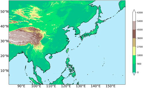
FIGURE 1. Model domain (the filled colours in the figure indicate terrain height).

2.2 Description of the case study

This study focused on two typical weather types in South China: 1) heavy summer rain and 2) cold winter spells. The cases were heavy rain from 1200 UTC 21 to 1200 UTC 24 May 2020 and cold spells from 0000 UTC 27 to 0000 UTC 30 December 2020. The mean circulation of heavy rain from ERA5 showed that South China was at the bottom of the deep trough of East Asia and behind the eastward short-wave trough (Figure 2A), which is a typical circulation for the rainstorms in South China (Xu et al., 2016). The mean circulation of winter cold spells is characterised by a low-pressure trough and cold tongue overlap in most of the country, with dense isothermal lines in South China (Figure 2B), which is also a typical circulation of cold spells. Therefore, we selected these two typical weather types to evaluate the simulation of thermal equilibrium characteristics in the South China Sea and surrounding areas using TRAMS.

FIGURE 2

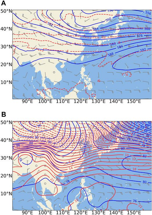
FIGURE 2. Mean circulation from ERA5 reanalysis data. (A) 500 hPa of summer heavy rain; (B) 925 hPa of winter cold spell. Potential height (blue line, dgpm, temperature (red line, °C); wind (vector, m/s).

2.3 Method

According to the method proposed by Klinker and Sardeshmukh (1992), during data assimilation, analysis at the previous time i-1 and the state of the atmosphere of this forecast at the lead time $\left(∆X_{\mathrm{i}}\right)$ are used to initialise the “first-guess” forecast $\left(F{C}_{\mathrm{i}}\right)$:

$F{C}_{\mathrm{i}}\equiv A{N}_{\mathrm{i}-1}+∆X_{\mathrm{i}}.(1)$

The analysis increment $\left(IN{C}_{\mathrm{i}}\right)$ is derived by “optimally combining” information from various observations and then adding it to the first-guess forecast. The updated analysis at time i $\left(A{N}_{\mathrm{i}}\right)$ is calculated as follows:

$A{N}_{\mathrm{i}}=F{C}_{\mathrm{i}}+IN{C}_{\mathrm{i}}.(2)$

Although the new observations have errors and cannot completely describe the atmospheric state, if the new analysis is closer to the truth than the first-guess forecast, these increments can be informative in identifying the model errors. The forecast error ($F{E}_{\mathrm{i}}$) during mode integration can be derived from Eqs 1, 2 as

$F{E}_{\mathrm{i}}\equiv F{C}_{\mathrm{i}}-A{N}_{\mathrm{i}}\left(=-IN{C}_{\mathrm{i}}\right)=A{N}_{\mathrm{i}-1}+∆X_{\mathrm{i}}-A{N}_{\mathrm{i}}.(3)$

Hence, the forecast error is considered negative for the increment. If the observation and first-guess forecast are exactly correct, then the increment is zero. Assuming that the observation errors are random and that the sample is sufficient, the mean observation error is zero. Thus, the non-zero analysis increment is due to errors in the model’s representation of the atmosphere’s dynamic or physical processes.

By averaging Eq. 3 over n consecutive analysis cycles and with $\overline{Y}=\frac{{\sum }_{\mathrm{i}=1}^{\mathrm{n}}{Y}_{\mathrm{i}}}{\mathrm{n}}$,

$\overline{FE}=-\overline{INC}=\overline{\Delta X}-\frac{A{N}_{\mathrm{n}}-A{N}_0}{\mathrm{n}}.(4)$

The term $\frac{A{N}_{\mathrm{n}}-A{N}_0}{\mathrm{n}}$ is the evolution of the flow over the time span of n analysis cycles. Depending on the length of n, this can include the daily or annual of the atmosphere. However, we assume that this term is negligible relative to the forecast error.

Considering the first-guess forecast as an average tendency over the time window $\left(\overline{\dot{X}}=\frac{\overline{\Delta X}}{\Delta t}\right)$ and decomposing it into the contribution from each process represented in the model (Cavallo et al., 2016),

$\overline{FE}=-\overline{INC}\approx \overline{\dot{X}}\Delta t=\left({\overline{\dot{X}}}_{Dyn}+{\overline{\dot{X}}}_{Rad}+{\overline{\dot{X}}}_{Gwd}+{\overline{\dot{X}}}_{Vdif}+{\overline{\dot{X}}}_{Conv}+{\overline{\dot{X}}}_{Cloud}+\dots +{\overline{\dot{X}}}_{res}\right)\Delta t,(5)$

where the right-hand brackets of the equation indicate the dynamics, radiation, gravity spell drag, vertical diffusion, convection, cloud, and other residential tendencies. The last term in the mean is usually ignored. Eq. 5 implies the theoretical correspondence of the model tendency and error, and the systematic forecast bias of the model can be regarded as the deviation of the net tendency with respect to the equilibrium state (net tendency equal to 0); while the dynamical core and physics schemes of the model should be in a quasi-equilibrium state in the ideal case, the deviation of the forecast tendency with respect to 0 (net tendency) can be used to assess the overall equilibrium features of the model. By decomposing the net forecast tendencies into the dynamical and each physical tendency, their contributions to simulations under different weather conditions can be further estimated.

3 Comparative analysis of moisture and temperature tendencies

Because of the weak baroclinicity of the tropical weather system in the South China Sea and its surrounding area, the convective instability energy mainly comes from the latent heat released by the condensation of warm and humid airflow in the lower troposphere. Therefore, we mainly discuss the thermal equilibrium characteristics of the TRAMS model from the perspective of temperature and water vapour. The moisture ($\overline{q}$) and temperature ($\overline{T}$) tendencies of the dynamical and each physical parameterisation scheme during model integration can be written as

$\frac{\partial \overline{T}}{\partial t}=\underset{Dyn}{\underbrace{-\overline{u}\frac{\partial \overline{T}}{\partial x}-\overline{v}\frac{\partial \overline{T}}{\partial y}-\overline{w}\frac{\partial \overline{T}}{\partial z}}}+Bl+Conv+Cloud+Rad,(6)$

$\frac{\partial \overline{q}}{\partial t}=\underset{Dyn}{\underbrace{-\overline{u}\frac{\partial \overline{T}}{\partial x}-\overline{v}\frac{\partial \overline{T}}{\partial y}-\overline{w}\frac{\partial \overline{T}}{\partial z}}}+Bl+Conv+Cloud,(7)$

where $\left(\overline{u},\overline{v},\overline{w}\right)$ are the three-dimensional wind field and Bl, Conv, Cloud, and Rad are the source-sink terms of the boundary layer, cumulus convection, cloud microphysical, and radiation parameterisations, respectively. The first three terms on the right-hand side of Eqs 6, 7 represent the advection process in the grid scale, which corresponds to the tendency of the dynamical core. According to the aforementioned two equations, the thermodynamic balance characteristics and contributions of each component in various weather systems can be determined.

3.1 Analysis of moisture and temperature tendencies from dynamic and total physics

First, the tendencies of each integration step are summed to get 72-h accumulated tendencies. Second, the regional average of the accumulated tendencies is calculated. Finally, we add the averaged tendencies of the dynamic (Dyn) and the physical (Phy) processes to obtain the net forecast tendencies (Net) (Figure 3).

FIGURE 3

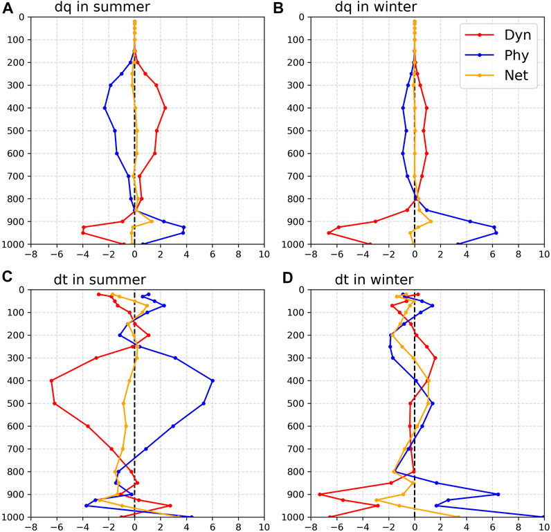
FIGURE 3. Regional average vapour and temperature tendencies. (A) Summer vapour tendency. (B) Winter vapour tendency. (C) Summer temperature tendency (°C). (D) Winter temperature tendency; dynamic process tendency (red line), physical process tendency (blue line), and net tendency (yellow).

The deviations in moisture tendencies are mainly concentrated below 200 hPa (troposphere) in both summer and winter (Figures 3A,B). Regardless of the season, because of water vapour transport from the near-surface by the vertical movement of the grid-scale (the third term on the right side of Eq. 7), the dynamic tendencies of moisture exhibit negative values near the surface, while showing a vertically extended positive value in the middle and upper troposphere, with a maximum at 950 hPa in summer (−4 × 10⁻³ g/kg) and winter (−7 × 10⁻³ g/kg). The physical and dynamic tendencies are roughly the opposite. The positive physical tendencies in the lower layers are attributed to the upward diffusion of evaporated water vapour from the near-surface and the evaporation of raindrops, whereas the negative physical tendencies in the middle and upper layers are mainly attributed to the water vapour condensation of the cumulus convection and cloud microphysical parameterisation. However, a net moisture tendency imbalance remains, with relatively obvious positive values from 925 to 700 hPa in both summer and winter, which suggests that the TRAMS overestimates moisture at 925–700 hPa in the South China Sea and its surrounding areas, with the same maximum value at 900 hPa (1 × 10⁻³ g/kg).

The temperature tendencies differed between summer and winter (Figures 3C,D), with deviations mainly below 250 hPa in summer and below 800 hPa in winter. During summer, the convection is relatively strong and deep; thus, the physical tendency is mainly positive in the middle and upper troposphere, with a maximum at 400 hPa (6°C) for strong latent heat release. Meanwhile, the dynamic process transports heat from the South China Sea and its surrounding regions to the middle and high latitudes through Hadley circulation and then reach temperature equilibrium. In the lower troposphere, the positive dynamic tendency originates from the warm and humid airflow brought by the southerly wind, while the negative physical tendency is mainly caused by the evaporation of raindrops, which absorb the heat from the atmosphere. In winter, the convection is relatively weak and shallow, resulting in a smaller positive physical tendency in the middle troposphere at 400–100 hPa. However, the negative tendency of the dynamic process near the surface, with a maximum at 900 hPa (6.5°C), mainly originates from the cold advection, and the greater temperature differences between the sea surface and atmosphere cause the physical process to deeply heat the lower atmosphere. The dynamic and physical tendencies are inverse between summer and winter, as discussed later.

Under the joint effect of dynamic and physical processes, the net temperature tendencies showed a negative bias in the forecast temperature in the lower troposphere, with a maximum value (-3°C) at 925 hPa in the simulation of the South China Sea and its surrounding areas during summer. The differences in temperature tendencies between summer and winter are centered at 600–300 hPa, whereas positive tendencies are observed in winter. In addition, the temperature deviation above the tropopause mainly originates from the mode dynamical core, which may be related to the low top height of the model.

The comparison between summer and winter showed that the moisture and temperature tendency deviations were mainly concentrated in the middle troposphere during the summer and in the lower troposphere during the winter. The similarity in the simulation errors of moisture and temperature between summer and winter at the lower troposphere may be the result of systematic bias in the model due to shallow or weak convection. Thus, the consumption of water vapour is low and the release of latent heat is insufficient, resulting in a cold and wet lower layer. However, the differences in the simulation errors, especially those in the middle troposphere during winter, may originate from the bias in the response of the physical parameterisation schemes, which will be discussed in the next section.

3.2 Analysis of moisture and temperature tendencies for individual physical processes

The regional average moisture tendencies from the boundary layer (BL), cumulus convection (Conv), and cloud microphysical (Cloud) processes are shown in Figures 4A,B. The variation trends in moisture tendencies for each physical process were similar in the summer and winter. The vapour in the lower troposphere mainly comes from water evaporation from the ground and sea surface. Therefore, the moisture regional average tendencies of the boundary layer process were mainly positive, with the same maximum at 925 hPa in both summer and winter (9 × 10⁻³ g/kg). The high temperature and humidity in the lower troposphere enhance low-level instability and favour convection that transports vapour upward further. Hence, the regional average moisture tendencies of the cumulus convection process were mainly negative throughout the troposphere, reaching the same minimum at 950 hPa (5×10⁻³ g/kg) in both summer and winter.

FIGURE 4

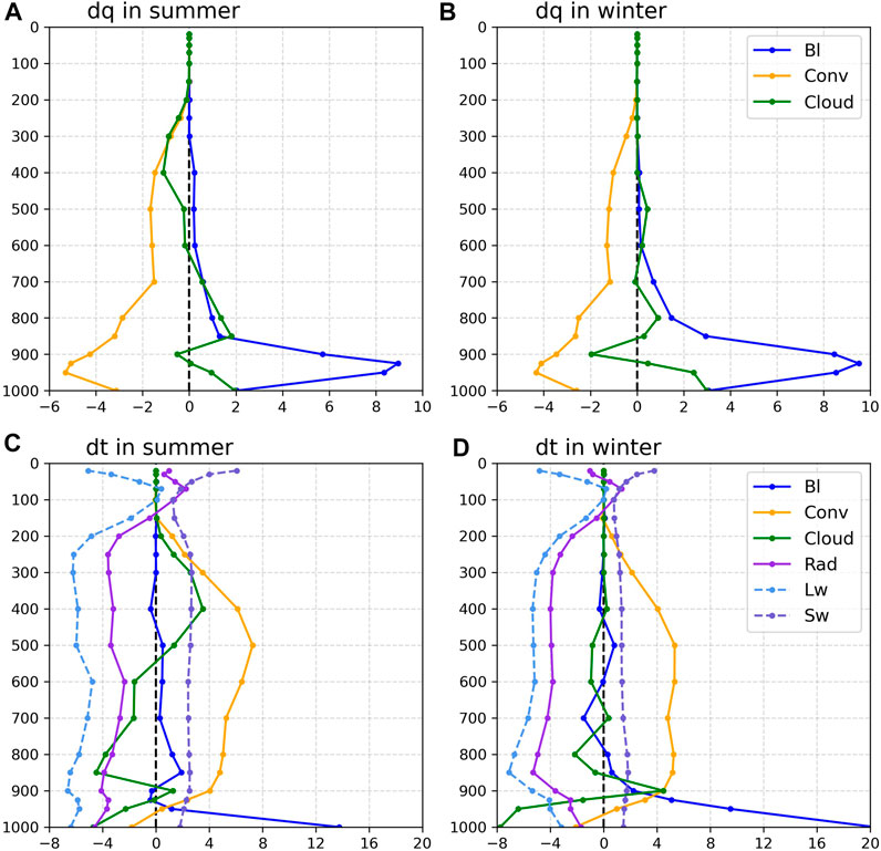
FIGURE 4. Regional average vapour and temperature tendencies from each physical scheme. (A) Summer vapour tendency (10⁻³ g/kg). (B) Winter vapour tendency (10⁻³ g/kg). (C) Summer temperature tendency (°C). (D) Winter temperature tendency (°C).

Generally, the stronger the deep convection, the higher the cloud. Hence, the moisture tendency in the cloud microphysical process is mainly negative for vapour condensation in the upper troposphere and positive for water evaporation in the middle and lower troposphere during summer. This occurs mainly in the lower troposphere during winter due to weak convection.

The regional average temperature tendencies of the boundary layer (BL), cumulus convection (Conv), cloud microphysical (Cloud), radiation (Rad), long-wave radiation (Lw) process, and short-spell radiation (Sw) processes are shown in Figures 4C,D. The heat from the ground and sea surface has a moderating effect on the temperature near the surface; therefore, the boundary layer process mainly contributed positively to the temperature at the low level, reaching a maximum at 1000 hPa in both summer (14°C) and winter (20°C). However, a negative tendency was also observed at 800–600 hPa in winter, which may be related to the turbulent entrainment process near the tops of stratocumulus clouds. During the cumulus convection process, the lifted vapour condenses and releases latent heat, which heats the atmosphere. Therefore, the temperature tendencies are mainly positive, with a maximum at 500 hPa in summer (7°C) and winter (5°C).

Vapour condensation releases heat and increases the temperature, and water evaporation absorbs heat and decreases the temperature. In the cloud microphysical process, the temperature is influenced by the phase change of the vapour. Hence, the temperature and moisture tendencies of the cloud microphysical process are approximately inverse. The troposphere is mostly cooled by long-wave radiation and heated by short-wave radiation. The long-wave radiation temperature tendencies are 2–3 times higher than those of short-wave radiation; therefore, the radiation process mainly cools the atmosphere. Above the boundary layer, the tendencies of the radiation and convection processes are almost in equilibrium.

In conclusion, the contributions of each physical process to the thermal equilibrium simulated by the TRAMS are generally reasonable in the South China Sea and surrounding areas. The regional average moisture and temperature tendencies of each physical process reveal that the boundary layer parameterisation always has positive contributions to moisture and temperature in the lower troposphere by transporting water vapour and heat from the near-surface to the lower troposphere. The cumulus convection parameterisation has negative contributions to moisture and temperature in the lower troposphere to further transport water vapour and heat, whereas it has a negative contribution to moisture and a positive contribution to temperature for water vapour condensation and latent heat release. The cloud microphysical parameterisation has positive contributions to moisture and negative contributions to temperature for water evaporation and heat absorption and opposite contributions to the middle and upper troposphere for water vapour condensation and latent heat release. However, the contribution altitude of cloud microphysical parameterisation differs between winter and summer owing to the convection.

In addition, the negative temperature tendencies in summer and bias of temperature tendencies from 900 to 300 hPa in winter mainly come from the radiation parameterisation, which may be affected by the cumulus convection and cloud microphysical parameterisation (cf. Figures 3,4) because water vapour absorbs long-wave radiation to heat the atmosphere and clouds reduce short-wave radiation absorption to cool the atmosphere. Additionally, the inverse temperature tendencies of the dynamic and physical tendencies originate from the height of the cloud microphysics latent heat release and heating influence of the boundary layer (cf. Figures 3C,D,4C,D,5E,F).

FIGURE 5

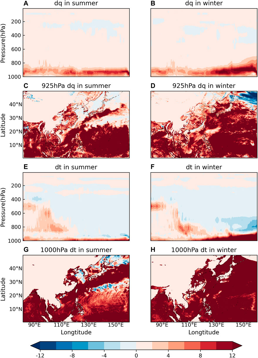
FIGURE 5. Vapour and temperature tendencies of the boundary layer process. (A–D) Vapour tendency (10–3 g/kg). (E–H) Temperature tendency (°C). (A,E) Latitudinal average cross-section in the summer. (B,F) Latitudinal average cross-section in the winter. (C) 925 hPa in the summer. (D) 925 hPa in the winter. (G) 1000 hPa in the summer. (H) 1000 hPa in the winter.

3.3 Further analysis of moisture and temperature tendencies from BL, Conv, and Cloud

Next, we analysed the latitudinal average and horizontal patterns with an apparent deviation of the boundary layer, cumulus convection, and cloud microphysical processes, which have a major effect on moisture and temperature predictions.

The moisture and temperature tendencies of the boundary layer process were mainly observed in the lower troposphere in both cases, especially over the ocean and coastal areas (Figure 5), which are mainly influenced by turbulent diffusion. During the summer, vapour and heat are mainly observed over Kuroshio and the downwelling area controlled by the WPSH (Figure 5C). In addition, a positive temperature tendency was observed at the bottom of the troposphere (Figure 5E). During the winter, the atmosphere energy mainly comes from the ocean; thus, the boundary layer process has a wider and higher influence on moisture and temperature compared to that in the summer, especially in the mid-latitudes, where the temperature differences between the sea surface and atmosphere are large. In addition, the warm and moist air was lifted by the topography of the Tibetan Plateau to condense and release latent heat near the height of 500 hPa at 80°E–120°E (Figures 5E,F). A comparison of net temperature tendencies revealed that the positive tendencies near the surface may be attributed to the overestimation of the sea surface heat flux by the boundary layer parameterisation (cf. Figures 3C,D,5E,F), which is consistent with the conclusion reported by Cavallo et al. (2016).

The moisture and temperature tendencies of the cumulus convection process are displayed in Figure 6. By transporting vapour and heat from the surface, the boundary layer process potentially enhance instability in the lower troposphere and favour the development of convection, which further transports vapour upward and heats the atmosphere with latent heat. Thus, the value of the tendencies is higher in summer owing to the more vigorous and deeper convection. Furthermore, a southwest–northeast zone with relatively obvious temperature tendencies is observed in South China during the summer (Figure 6G), corresponding to the rainfall zone. While related to the deviation of temperature tendencies, once the deep convection is triggered, the consumption of vapour and formation of clouds reduces the absorption of both long-wave and short-wave radiation and cools the atmosphere.

FIGURE 6

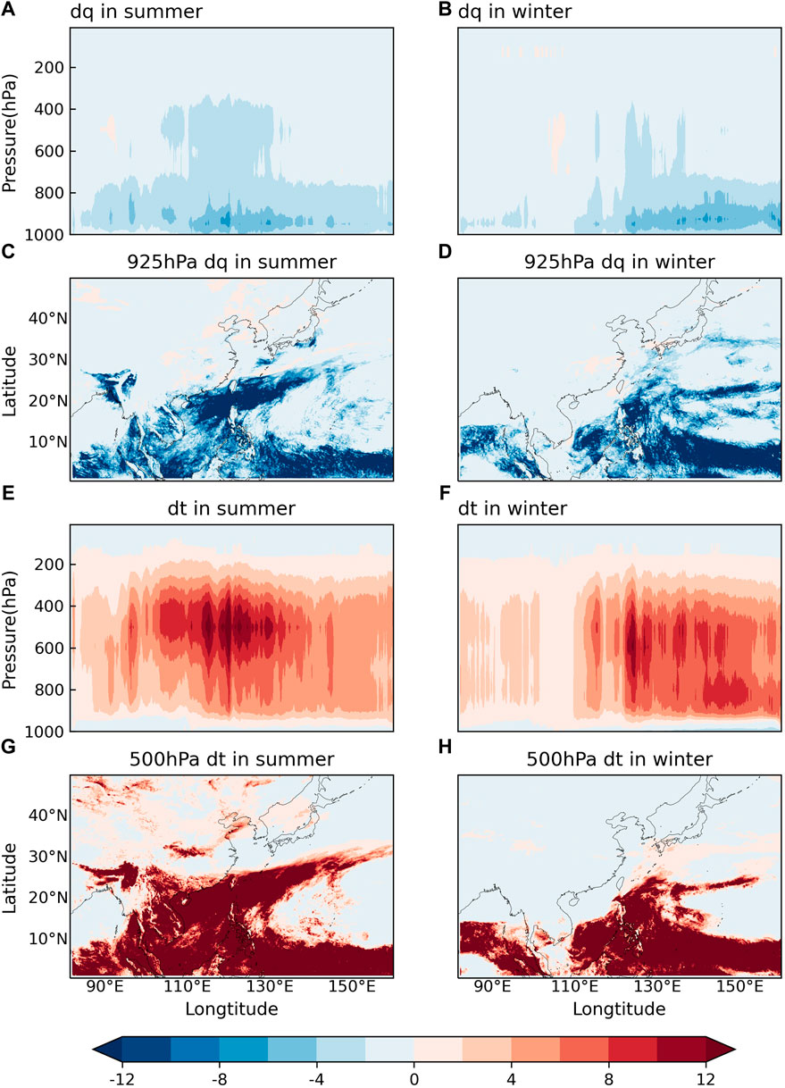
FIGURE 6. Vapour and temperature tendencies of the cumulus convection process. (A–D) Vapour tendency (10–3 g/kg). (E–H) Temperature tendency (°C). (A,E) Latitudinal average cross-section in the summer. (B,F) Latitudinal average cross-section in the winter. (C) 925 hPa in the summer. (D) 925 hPa in the winter. (G) 500 hPa in the summer. (H) 500 hPa in the winter.

In the cloud microphysical process, the moisture tendencies are mainly negative (Figures 7A,B), and the temperature tendencies are usually positive (Figures 7E,F) when vapour condenses into drops and ice in the cloud after lifting to the condensation height by convection. The clouds are usually higher and more widespread in summer but be lower and concentrated over the ocean in winter. Moisture and temperature tendencies are mainly affected by the WPSH in summer and the deep trough of East Asia in winter (cf. Figures 2, 7C,D,G,H). The warm and moist airflow brought by the southwesterly wind meets the cold and dry airflow moving southward at the northern branch of the WPSH, which is conducive to the convergence of vapour and the formation of clouds and rain. The deep trough of East Asia is also favorable for the upward movement and condensation of vapour. The moisture tendencies of the cloud microphysical process are mainly observed above the ocean in winter but expand to land in summer because of the westward extension of the WPSH. A comparison of net moisture tendencies showed that the positive tendencies in the lower troposphere may occur due to the underestimation of vapour consumption by the cloud microphysical parameterisation (cf. Figures 3A,B,5E,F).

FIGURE 7

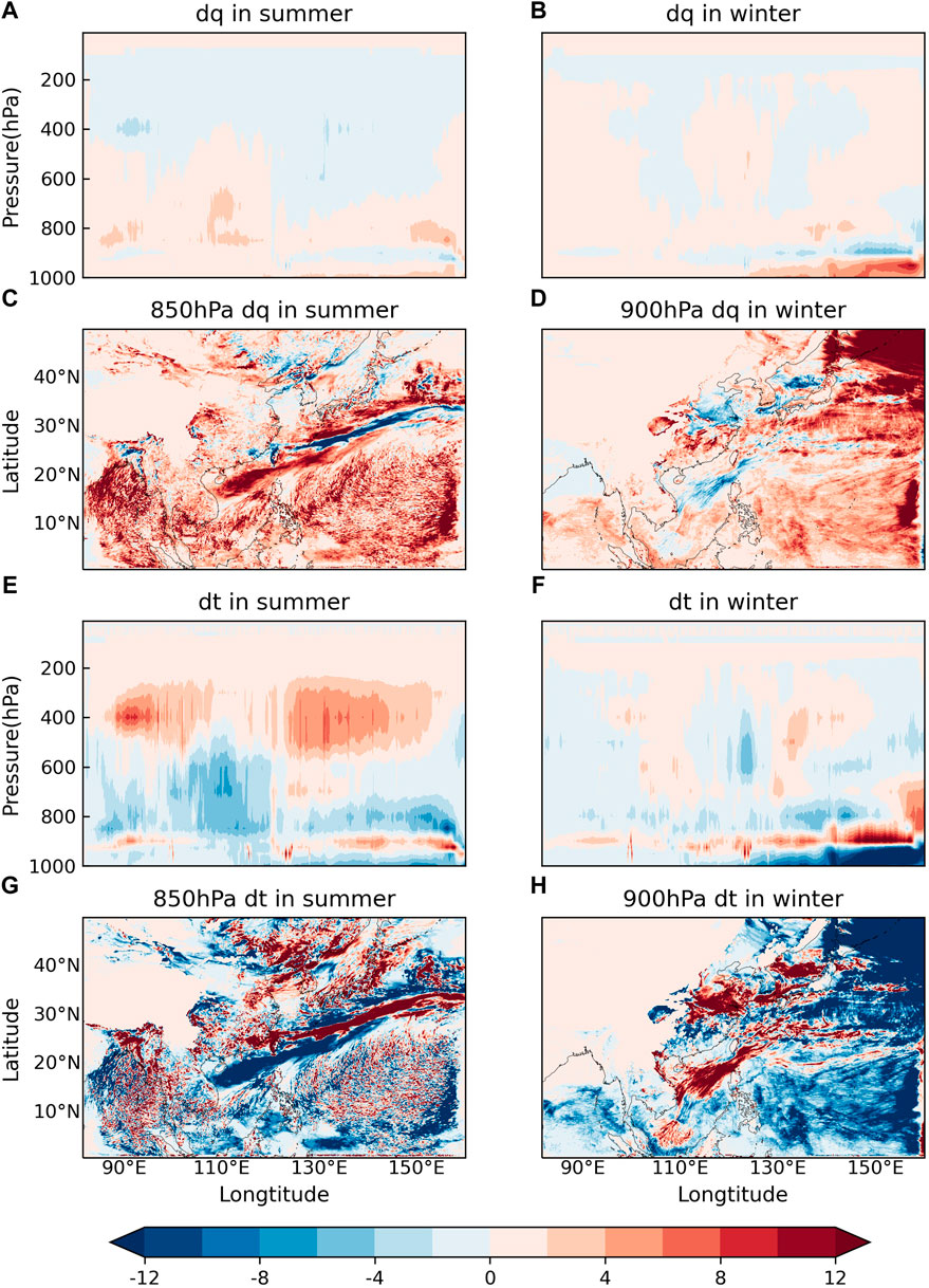
FIGURE 7. Vapour and temperature tendencies of the cloud microphysical process. (A–D) Vapour tendency (10–3 g/kg). (E–H) Temperature tendency (°C). (A,E) Latitudinal average cross-section in the summer. (B,F) Latitudinal average cross-section in the winter. (C) 850 hPa in the summer. (D) 900 hPa in the winter. (G) 850 hPa in the summer. (H) 900 hPa in the winter.

The boundary layer process transports vapour and energy to the lower troposphere via turbulent diffusion and is conducive to the development of convection. After lifting to the condensation height by convection, vapour condenses and is partly converted into raindrops and ice in the cloud in the cumulus convection and cloud microphysical processes, which heats the atmosphere through latent heat. Therefore, the WPSH and deep trough of East Asia, which favour the upward and convergence of airflow, primarily affect the moisture and temperature in the simulation of the South China Sea and its surrounding areas.

The results show that the underestimation of the vapour consumption by cloud microphysical parameterisation and the overestimation of the sea surface heat flux by boundary layer parameterisation yield relatively high moisture and temperature in the lower troposphere. The temperature forecast bias from 900 to 300 hPa is mainly caused by the responses of radiation, cumulus convection, and cloud microphysical parameterisations.

4 Correlation of moisture and temperature regional average tendencies from dynamic and physics

To further analyse the interactions of the dynamic and each physical process, we calculated the correlation coefficients of the regional average moisture and temperature tendencies from the dynamic and each physical process (each fold in Figure 4).

The boundary layer and cumulus convection processes showed major contributions to the moisture tendencies in both summer and winter and were always anti-correlated, with correlation coefficients as high as 0.882 in summer and 0.908 in winter (Tables 1,2). In addition, the obvious positive correlation between vapour (Qv) and water (Qc) in the cloud microphysical process during summer (correlation coefficient 0.617) suggested the important role of the warm cloud process in the cloud microphysical process.

TABLE 1

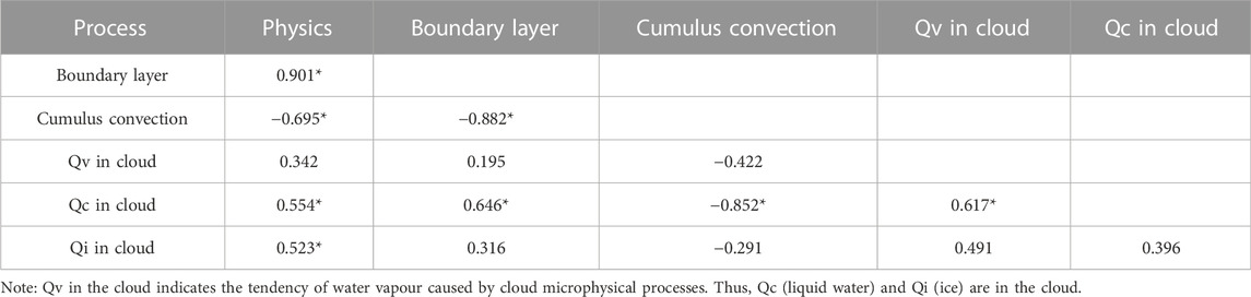
TABLE 1. Correlation coefficients of the vapour tendencies for each process in the summer.

TABLE 2

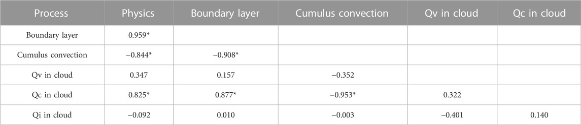
TABLE 2. Correlation coefficients of the vapour tendencies for each process in the winter.

None of the physical processes is significantly correlated with the total physical process in summer, and only the boundary layer process showed significant effects on temperature prediction in winter (Tables 3,4). The correlation coefficients of the boundary layer and the total physical processes in winter were larger than those in summer because the ground and ocean are the main sources of heat. In addition, the inverse relationship between the radiation process and cumulus convection process in winter also supported the idea that vapour consumption and cloud formation reduce the absorption of both long-wave and short-wave radiation and cool the atmosphere. Furthermore, their correlation coefficient was not low in the summer, although the difference was not statistically significant.

TABLE 3

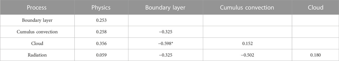
TABLE 3. Correlation coefficients of the temperature tendencies for each process in the summer.

TABLE 4

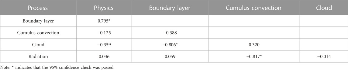
TABLE 4. Correlation coefficients of the temperature tendencies for each process in the winter.

The boundary layer and cumulus convection processes contribute markedly to moisture and temperature prediction. Their interactions are important for the simulation of the thermal equilibrium. The importance of the boundary layer process can be inferred from its significant correlations with both temperature and moisture. In addition, the inverse relationship between the radiation and cumulus convection processes also supports the idea that the reduction of vapour by deep convection is favourable for radiation cooling.

5 Conclusion and discussion

Focusing on two typical weather types in the South China Sea and its surrounding areas, this study evaluated the thermal equilibrium simulated by the TRAMS in terms of forecast tendencies. By examining the contributions of the dynamic and each physical process, we identified the sources of simulation biases and provide a reference for further optimisation and improvement of the model. The conclusions are as follows.

1) The equilibrium characteristics of the model simulation are generally reasonable, showing that the dynamic and physical processes have opposite trends and largely balance each other. Consistent with the actual situation, moisture and temperature departures are mainly concentrated in the middle troposphere during the summer and in the lower troposphere during the winter.

2) The contributions of each physical process to the thermal equilibrium are generally reasonable; however, the differences between summer and winter are marked. The results showed that the underestimation of vapour consumption by cloud microphysical parameterisation and the overestimation of sea surface heat flux by the boundary layer parameterisation near the surface dominate the systematic bias of the model. The temperature bias from 900 hPa to 300 hPa during the winter mainly originates from the responses of radiation, cumulus convection, and cloud microphysical parameterisations. Water vapour absorbs long-wave radiation to heat the atmosphere, whereas clouds reduce short-wave radiation absorption to cool the atmosphere.

3) The WPSH and deep trough of East Asia, which are conducive to uplift and convergence, primarily affected the difference in each physical parameterisation response between summer and winter in the simulation of the South China Sea and its surrounding areas.

This study mainly focused on the evaluation of thermal equilibrium in the troposphere. However, relatively distinct deviations occur near the surface and above the stratosphere, the causes of which remain unclear. Furthermore, this study only analysed the thermal equilibrium of the dynamic and physical processes and the interaction of each physical process. Several other equilibria require further evaluation in this model. Studies are needed to compare the tendencies of the TRAMS to the standard tendency data provided by the Year of Tropical Convection (YOTC) project (Moncrieff et al., 2012) to analyse the deviation of each process and further evaluate its impact on the forecast.

Data availability statement

This study analyzed publicly available datasets. These data can be found at https://cds.climate.copernicus.eu/cdsapp#!/home.

Author contributions

SZ was responsible for the study conception, manuscript writing, and figure development. FX, BZ and YX provided guidance and funding support. DX and JC-HL were responsible for discussion and manuscript revision. LH, JY, MZ, YL, and FH were contributed to the conception and design of the work.

Funding

This study was supported by the Special Project for Research and Development in Key area of Guangdong Province (Grant 2020B0101130021) and the National Key Research and Development Program of China (Grant 2018YFC1506902).

Acknowledgments

We thank the Guangzhou Institute of Tropical Marine Meteorology of the China Meteorological Administration for providing the facilities to conduct the numerical analysis.

Conflict of interest

The authors declare that the research was conducted in the absence of any commercial or financial relationships that could be construed as a potential conflict of interest.

Publisher’s note

All claims expressed in this article are solely those of the authors and do not necessarily represent those of their affiliated organizations, or those of the publisher, the editors, and the reviewers. Any product that may be evaluated in this article, or claim that may be made by its manufacturer, is not guaranteed or endorsed by the publisher.

References

Arakawa, A., and Schubert, W. H. (1974). Interaction of a cumulus cloud ensemble with the large-scale environment, Part I. J. Atmos. Sci. 31 (3), 674–701. doi:10.1175/1520-0469(1974)031<0674:ioacce>2.0.co;2

CrossRef Full Text | Google Scholar

Cavallo, S. M., Berner, J., and Snyder, C. (2016). Diagnosing model errors from time-averaged tendencies in the weather research and forecasting (WRF) model. Mon. Weather Rev. 144 (2), 759–779. doi:10.1175/mwr-d-15-0120.1

CrossRef Full Text | Google Scholar

Chen, D.-H., Xue, J.-S., Yang, X.-S., Zhang, H.-L., Shen, X.-S., Hu, J.-L., et al. (2008). New generation of multi-scale NWP system (GRAPES): General scientific design. Sci. Bull. (Beijing). 53 (22), 3433–3445. doi:10.1007/s11434-008-0494-z

CrossRef Full Text | Google Scholar

Chen, X.-J., Liu, Q.-J., and Ma, Z.-S. (2021). A diagnostic study of cloud scheme for the GRAPES global forecast model. Acta Meteorol. Sin. (in Chin.) 79 (01), 65–78. doi:10.11676/qxxb2020.066

CrossRef Full Text | Google Scholar

Chen, Z.-T., Dai, G.-F., Luo, Q.-H., Zhong, S.-X., Zhang, Y.-X., Xu, D.-S., et al. (2016). Study on the coupling of model dynamics and physical processes and its influence on the forecast of typhoons. J. Trop. Meteorology 32 (01), 1–8. doi:10.16032/j.issn.1004-4965.2016.01.001

CrossRef Full Text | Google Scholar

Crawford, W., Frolov, S., McLay, J., Reynolds, C. A., Barton, N., Ruston, B., et al. (2020). Using analysis corrections to address model error in atmospheric forecasts. Mon. Weather Rev. 148 (9), 3729–3745. doi:10.1175/mwr-d-20-0008.1

CrossRef Full Text | Google Scholar

Droegemeier, K. K., Xue, M., Reid, P. V., Straka, J., Bradley, J., and Lindsay, R. (1991). The advanced regional prediction system (ARPS) version 2. 0: Theoretical and numerical formulation. Oklahoma: Center for Analysis and Prediction of Storms Rep. CAPS91-001, 55.

Google Scholar

Dudhia, J. (1996). The Sixth PSU/NCAR mesoscale model users’ workshop. Boulder, CO, USA: National Center for Atmospheric Research, 49–50. A multi-layer soil temperature model for MM5.

Google Scholar

Han, J., and Pan, H.-L. (2011). Revision of convection and vertical diffusion schemes in the NCEP global forecast system. Weather Forecast. 26 (4), 520–533. doi:10.1175/WAF-D-10-05038.1

CrossRef Full Text | Google Scholar

Hong, S.-Y., Dudhuia, J., and Chen, S.-H. (2004). A revised approach to ice microphysical processes for the bulk parameterization of clouds and precipitation. Mon. Weather Rev. 132 (1), 103–120. doi:10.1175/1520-0493(2004)132<0103:aratim>2.0.co;2

CrossRef Full Text | Google Scholar

Hong, S.-Y., and Pan, H.-L. (1996). Nonlocal boundary layer vertical diffusion in a medium-range forecast model. Mon. Weather Rev. 124 (10), 2322–2339. doi:10.1175/1520-0493(1996)124<2322:nblvdi>2.0.co;2

CrossRef Full Text | Google Scholar

Iacono, M. J., Delamere, J. S., Mlawer, E. J., Shephard, M. W., Clough, S. A., and Collins, W. D. (2008). Radiative forcing by long-lived greenhouse gases: Calculations with the AER radiative transfer models. J. Geophys. Res. 113 (D13), D13103. doi:10.1029/2008JD009944

CrossRef Full Text | Google Scholar

Kay, J. E., Raeder, K., Gettelman, A., and Anderson, J. (2011). The boundary layer response to recent arctic sea ice loss and implications for high-latitude climate feedbacks. J. Clim. 24 (2), 428–447. doi:10.1175/2010jcli3651.1

CrossRef Full Text | Google Scholar

Klinker, E., and Sardeshmukh, P. D. (1992). The diagnosis of mechanical dissipation in the atmosphere from large-scale balance requirements. J. Atmos. Sci. 49 (7), 608–627. doi:10.1175/1520-0469(1992)049<0608:tdomdi>2.0.co;2

CrossRef Full Text | Google Scholar

Klocke, D., and Rodwell, M. J. (2014). A comparison of two numerical weather prediction methods for diagnosing fast-physics errors in climate models. Q. J. R. Meteorol. Soc. 140 (679), 517–524. doi:10.1002/qj.2172

CrossRef Full Text | Google Scholar

Li, H.-R., Xu, D.-S., and Zhang, B.-L. (2021). Implementation of the incremental analysis update initialization scheme in the tropical regional atmospheric modeling system under the replay configuration. J. Meteorol. Res. 35 (1), 198–208. doi:10.1007/s13351-021-0078-2

CrossRef Full Text | Google Scholar

Lin, X.-X., Feng, Y.-R., Xu, D.-R., Jian, Y.-R., Huang, F., and Huang, J.-C. (2022). Improving the nowcasting of strong convection by assimilating both wind and reflectivity observations of phased array radar: A case study. J. Meteorol. Res. 36 (1), 61–78. doi:10.1007/s13351-022-1034-5

CrossRef Full Text | Google Scholar

Ma, Z.-S., Liu, Q.-J., and Qin, Y.-Y. (2016). Validation and evaluation of cloud and precipitation forecast performance by different moist physical processes schemes in GRPAES_GFS model. Plateau Meteorol. (in Chin.) 35 (04), 989–1003. doi:10.7522/j.issn.1000-0534.2015.00063

CrossRef Full Text | Google Scholar

Martin, G. M., Milton, S. F., Senior, C. A., Brooks, M. E., Ineson, S., Reichler, T., et al. (2010). Analysis and reduction of systematic errors through a seamless approach to modeling weather and climate. J. Clim. 23 (22), 5933–5957. doi:10.1175/2010jcli3541.1

CrossRef Full Text | Google Scholar

Moncrieff, M. W., Waliser, D. E., Miller, M. J., Shapiro, M. A., Asrar, G. R., and Caughey, J. (2012). Multiscale convective organization and the YOTC virtual global field campaign. Bull. Am. Meteorol. Soc. 93 (8), 1171–1187. doi:10.1175/BAMS-D-11-00233.1

CrossRef Full Text | Google Scholar

Phillips, T. J., Potter, G. L., Williamson, D. L., Cederwall, R. T., Boyle, J. S., Fiorino, M., et al. (2004). Evaluating parameterizations in general circulation models: Climate simulation meets weather prediction. Bull. Am. Meteorol. Soc. 85, 1903–1916.

CrossRef Full Text | Google Scholar

Rodwell, M. J., Jung, T., Bechtold, P., Berrisford, P., Bormann, N., Cardinali, C., et al. (2010). Developments in diagnostics research. Reading, England: ECMWF Technical Memorandum, 637.

Google Scholar

Rodwell, M. J., and Palmer, T. N. (2007). Using numerical weather prediction to assess climate models. Q. J. R. Meteorol. Soc. 133 (622), 129–146. doi:10.1002/qj.23

CrossRef Full Text | Google Scholar

Skamarock, W. C., Klemp, J. B., Dudhia, J., Gill, D. O., Barker, D. M., Wang, W., et al. (2008). A description of the advanced research WRF version 2. University Corporation for Atmospheric Research, Boulder, Colorado, United States,

Google Scholar

Torn, R. D., and Davis, C. A. (2012). The influence of shallow convection on tropical cyclone track forecasts. Mon. Weather Rev. 140 (7), 2188–2197. doi:10.1175/mwr-d-11-00246.1

CrossRef Full Text | Google Scholar

Williams, K. D., Bodas-Salcedo, A., Déqué, M., Fermepin, S., Medeiros, B., Watanabe, M., et al. (2013). The transpose-AMIP II experiment and its application to the understanding of southern ocean cloud biases in climate models. J. Clim. 26 (10), 3258–3274. doi:10.1175/jcli-d-12-00429.1

CrossRef Full Text | Google Scholar

Wong, M., Romine, G., and Snyder, C. (2020). Model improvement via systematic investigation of physics tendencies. Mon. Weather Rev. 148 (2), 671–688. doi:10.1175/mwr-d-19-0255.1

CrossRef Full Text | Google Scholar

Xu, D.-S., Zhang, B.-L., Zeng, Q.-C., Feng, Y.-R., Zhang, Y.-X., and Dai, G.-F. (2019). A typhoon initialization scheme based on incremental analysis updates technology. Acta Meteorol. Sin. 77 (6), 1053–1061. doi:10.11676/qxxb2019.060

CrossRef Full Text | Google Scholar

Xu, D.-S., Zhang, Y.-X., Wang, G., Meng, W.-G., and Chen, Z.-T. (2015). Improvement of meso-SAS cumulus parameterization scheme and its application in a model of 9 km resolution. J. Trop. Meteorology (in Chinese) 31 (5), 608–618. doi:10.16032/j.issn.1004-4965.2015.05.004

CrossRef Full Text | Google Scholar

Xu, M., Zhao, Y.-C., Wang, X.-F., and Wang, X.-K. (2016). Statistical characteristics and circulation pattern of sustained torrential rainduring the pre-flood season in South China for recent 53 years. Torrential Rain and Disasters 35, 109–118. doi:10.3969/j.issn.1004—9045.2016.02.003

CrossRef Full Text | Google Scholar

Yanai, M., Esbensen, S., and Chu, J.-H. (1973). Determination of bulk properties of tropical cloud clusters from large-scale heat and moisture budgets. J. Atmos. Sci. 30 (4), 611–627. doi:10.1175/1520-0469(1973)030<0611:dobpot>2.0.co;2

CrossRef Full Text | Google Scholar

Zhang, H., Lin, Z.-H., and Zeng, Q.-C. (2011). The mutual response between dynamical core and physical parameterizations in atmospheric general circulation models. Climatic and Environmental Research (in Chinese) 16 (01), 15–30. doi:10.3878/j.issn.1006-9585.2011.01.02

CrossRef Full Text | Google Scholar

Zhang, Y.-X., Chen, Z.-T., Meng, W.-G., and Xu, D.-S. (2022). Applicability of temperature discrete equation to NMRF boundary layer scheme in GRAPES model. jtm. 28 (1), 12–28. doi:10.46267/j.1006-8775.2022.002

CrossRef Full Text | Google Scholar