Mapping of the Subglacial Topography of Folgefonna Ice Cap in Western Norway—Consequences for Ice Retreat Patterns and Hydrological Changes

1 Introduction

Melting of mountain glaciers is currently contributing considerably to a global sea level rise (Zemp et al., 2019) and this is likely to continue throughout the 21^st century (Radić and Hock, 2011), as the cryosphere is rapidly changing due to ongoing global warming (Gulev et al., 2021). A rising sea level has implications for coastal societies (Hinkel et al., 2014), both in terms of the economy and the risk of geohazards (Nicholls, 2011; Hallegatte et al., 2013; Vitousek et al., 2017). Locally, mountain glaciers also remain buffers in the hydrological cycle, temporarily storing fresh water in high mountain areas (Bradley et al., 2006). Hence, in many countries, meltwater from glaciers is a stable source of water for drinking, farmland irrigation, and hydropower production (Nesje et al., 2008; Immerzeel et al., 2010; Kaser et al., 2010; Chevallier et al., 2011). In addition, mountain glaciers are important for the tourism industry, with unique opportunities for summer skiing and glacial hikes creating jobs for people living in rural areas. When these mountain glaciers now rapidly retreat they may cause geohazards, for example make the ground unstable for hikers (Purdie, 2013), or temporarily dam water that could lead to a glacial lake outburst flood (GLOF; Bajracharya and Mool, 2009). GLOFs have occurred in many places around the world, including at Folgefonna, and in areas such as Nepal, the Himalayas, the Andes, and the southern Alaska–Yukon ranges (e.g., Hewitt, 1982; Carrivick and Tweed, 2016; Cook et al., 2016; Cook et al., 2018). Local knowledge about how glaciers will retreat is vital to prepare and implement measures to counteract the negative effects of GLOFs. Knowledge of the ice thickness, and thus the subglacial topography, is important, as it is a necessary input for glaciological models that can be applied to assess past and future glacial fluctuations (Laumann and Nesje, 2014; Åkesson et al., 2017).

In this study we use ice-penetrating radar to map the subglacial topography of Sørfonna, the largest of the Folgefonna ice caps, which has only been partly mapped before (Brekke and Nord, 2008) and, is important for hydropower production in the country. The ability of radar to penetrate glacier ice has been known since the 1960s, when deviations in altimetry were observed during an attempted landing of an aircraft on the Greenland ice sheet. (Waite and Schmidt, 1961; Annan, 2003). Radar measurements are today used in several fields of earth science, and on glaciers they can be used to investigate snowpacks, glacial hydrology, ice thickness, subglacial topography and englacial properties (Pälli et al., 2002; Pettersson, 2003; Woodward and Burke, 2007; Yde et al., 2014; Magnússon et al., 2016).

Glaciological models are based on algorithms that describe parameters such as ice flow, bed friction, and internal deformation, which depend on detailed subglacial terrain models to be reliable. Because glacial advance and retreat are difficult to predict, most models are constricted to short-term (decadal or century) reconstruction or predictions (Åkesson et al., 2017). More advanced models require local measurements of radiation balance, albedo, temperature etc. that would require setting up a climate station to gather data for at least one season. In this study, we chose a model that uses data that we knew were available to get a good assessment of future glacial retreat in the study area. The model has already been proven to work well in previous studies on glaciers in western Norway (Laumann and Nesje, 2014). The datasets used are the subglacial topography map produced in this study, an existing digital elevation model (DEM) of the glacial surface, mass balance, temperature, and precipitation records.

The main objective for this paper is to map the subglacial topography of Sørfonna based on ice-penetrating radar measurements with low-frequency electromagnetic waves, and to combine this with previous results from the Foglefonna ice cap, Nordfonna (Førre, 2012), to present the first detailed map of the subglacial landscape under Folgefonna. Secondary objectives are (1) to use a dynamical ice flow model to assess the future melting of the glacier based on two climate scenarios (one with a 1.5°C warming and a 3% increase in precipitation, and a second with a 3.5°C warming together with 15% increase in precipitation), (2) to provide detailed analyses of the hydrological changes (such as drainage catchments extent) that will take place in the landscape as the glacier melts, (3) to compare our findings with similar studies in Scandinavia and beyond, (4) to qualitatively discuss changes in drainage patterns based on numerous existing sediment records from lakes around Sørfonna for identifying bedrock thresholds that can redirect the meltwater drainage, and (5) to investigate the potential for future GLOFs as the glacier retreats over the next century.

2 Study Site

Folgefonna is the collective name of three temperate ice caps (Nordfonna, Midtfonna, and Sørfonna) located on the Folgefonna peninsula in a maritime setting in southwest Norway (Figure 1). More than 11,000 people live in this area and Folgefonna is surrounded by roads and other infrastructure. In 2005, the area was awarded national park status and received the name ‘Folgefonna National Park’. Sørfonna ice cap is the third largest glacier in Norway, with an area of about 164 km² (Andreassen et al., 2012). It is approximately 20 km long from north to south, about 2 km wide in the far north, and 12 km wide at its widest part in the south (Figure 1). Many of the outlet glaciers and the glacial valleys at Sørfonna and Nordfonna are important for the tourist industry today, with a history that goes back to the early 19^th century.

FIGURE 1

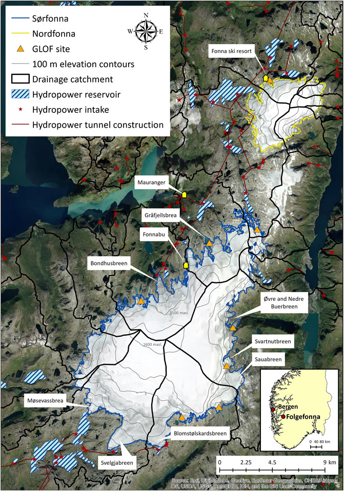
FIGURE 1. Nordfonna (yellow boundary) and Sørfonna (blue boundary), with 100 m elevation contours (thin grey lines) in the centre. Sites with potential or historically observed glacial lake outburst floods (GLOFs) are marked with orange triangles (Jackson and Ragulina, 2014; Norwegian Water Resources and Energy Directorate, 2017). Hydropower constructions are marked with red stars and lines, reservoirs are marked with blue stripes, and drainage basins are marked with black lines. The outlet glaciers mentioned in the manuscript are marked by their names. The inset map (bottom right; ©EuroGeographics for the administrative boundaries) shows where in southwestern Norway Folgefonna (red dot) is located.

Most of the meltwater draining from the northwest and south flanks of Sørfonna is used for hydropower production. Two hydropower companies, Statkraft AS and Sunnhordaland Kraftlag AS, have reservoirs located high in the mountains (> 900 masl.), which benefit from using the glacier as a natural storage facility or buffer. Hydropower with storage capacity is particularly useful because reservoirs serve as important tools to mitigate floods and droughts while generating energy. Having a glacier in the catchment yields another advantage: the water supply to the reservoir is secured, regardless of whether the summer is wet and cold or hot and dry, because the melting glacier compensates for the lack of precipitation during dry and warm summers. Both hydropower companies have made several modifications to the catchments’ drainage systems to meet their needs; for example, during the late 1960s and early 1970s, more than 100 km of tunnels were built to collect meltwater for high mountain storage (Statkraft AS, 2020). The meltwater is directed into underground plants, and the outlet leads directly to the fjord or a river system in which several river runoff power plants are in a cascade to optimize water use. For future adaptation of water runoff, it is crucial to better understand the possibilities for rerouting meltwater, as well as the risk of geohazards as the glacier retreats.

Based on historical evidence, several sites around Folgefonna are known to have caused GLOFs, and some of them have the potential to cause GLOFs in the future (Norwegian Water Resources and Energy Directorate, 2019; Figure 1). The outlet glacier Svartnutbreen has been linked to several documented GLOFs over the past 8,000 years, with the latest occurring in 2002 (Røthe et al., 2019). The small village of Mosnes in Åkrafjorden, to the south of Sørfonna, is an area that has been heavily affected by GLOFs in the recent past. Repeated flooding during the 1950s and 1960s from a lake formed on the side of the outlet glacier Sauabreen damaged houses and infrastructure, and the last permanent settlement was abandoned in 1966 (Jackson and Ragulina, 2014). There is no present GLOF threat to Mosnes, as the Sauabreen glacier has retreated and is therefore no longer creating a glacier-dammed lake (Tvede, 1989). Further northwest, glacier-dammed lakes can be found at Fyndersdalhorga and Gråfjellsbrea glacier (Jackson and Ragulina, 2014). There are also observations of GLOFs in the catchment north of Nordfonna, towards Jondal (Bakke et al., 2005). Based on these events, it is likely that areas subjected to GLOFs around the Sørfonna ice cap will shift in the future when outlet glaciers retreat and potentially dam up lakes in new areas.

The Folgefonna ice caps have decreased both in area and volume over the past two decades. For example, the outlet glacier Bondhusbreen (northwestern Sørfonna; Figure 1), retreated 290 m between 1959 and 2013 (Kjøllmoen, 2014), while the outlet glacier Svelgjabreen (southern Sørfonna; Figure 1), retreated 140–150 m between 1959 and 2017 (Kjøllmoen, 2018).

Using two meteorological stations along the fjord Hardangerfjorden (Ullensvang Forsøksgaård and Omastrand; Aune, 1993), the present mean summer temperature (Ts) from 1 May to 30 September is estimated to be 12.8°C at sea level along the fjord. With an environmental lapse rate of 0.68°C per 100 m (Sutherland, 1984), the mean Ts is close to 4.08°C at the modern equilibrium line altitude (ELA; 1465 masl.) at the Gråfjellsbrea outlet glacier (Figure 1). From 1961 to 1990, a local meteorological station 11 km north of Nordfonna (Kvale, 342 masl.; Førland, 1993) recorded the winter precipitation (Pw) from 1 October to 30 April, the mean of which was 1,434 mm. Based on an empirical, exponential increase in winter precipitation of 8% per 100 m (Haakensen, 1989), the corresponding Pw at the ELA of Nordfonna is about 3,350 mm. Snow measurements conducted by the Norwegian Water Resources and Energy Directorate (NVE) show that the Svelgjabreen outlet glacier (Figure 1) in the southern part of Sørfonna (Tvede and Liestøl, 1977; Østrem et al., 1988) has an estimated winter balance of more than 5,000 mm Pw, resulting in a gradient between 3,350 mm Pw in the north and 5,000 mm Pw in the south.

3 Methods

3.1 Radar Measurements, Processing, and Map Construction

Ice thickness measurements were collected by towing a Blue Systems ice-penetrating radar (Blue Systems Integration Ltd., 2013) with a low-frequency (2.5 MHz) antenna and an on-board GPS behind a snowmobile (about 20 km h⁻¹). The transmitter (Tx) and receiver (Rx) were in two different sledges in line with each other. The antenna arms were protected by flat PVC tubing. The spacing between Tx and Rx was 60 m, and each of the two antenna arm lengths was 16.8 m. Combined, the total drag after the snowmobile was about 120 m. There is a schematic figure of the radar setup in Supplementary Appendix S1.

The antenna spacing was tested in the field, and 60 m proved to be the optimal distance for a clear reading. The signal’s vertical range was set to 50 mV, and the sampling rate was set to 250 MHz. The trigger selection edge regulated the level (mV) at which the measurement should be triggered (trigger level). The trigger level was set to 40 mV, but it had to be adjusted a few times in the field to trigger the measurement. Both 5 and 10 MHz antennas were tested, but they proved insufficient for penetrating to the bedrock in large regions where the ice thickness exceeded about 100 m, probably due to the high water content in the ice (Rignot et al., 2013). Profiles measuring the transition from the ice edge to thicker ice (about 50 m) were collected using a Malå ground penetrating radar (GPR) system with a 25 MHz Rough Terrain Antenna (RTA) series antenna with a 12 channel GPS (± 5 m accuracy). Data from Sørfonna were collected for 5 days in March of each year from 2015 to 2018. The data were collected in a grid, with longitudinal spacing of 500 m (NE-SW) and transverse spacing of 1,000 m (NW-SE). Data from Nordfonna were collected by Førre (2012). Post-processing and analysis of the radar profiles were conducted using Reflexw software (Sandmeier, 2016) with standard radar processing tools (e.g., interpolation of GPS measurements to all traces, trace interpolation and removal of standstill traces, static correction, application of an AGC gain filter, equidistance traces, Stoltz migration, and time-to-depth conversion).

The precision of the ice thickness dataset was investigated by comparing ice thickness measurements at all locations where radar profiles crossed (i.e., crossover analysis). The radar GPS elevations were compared to a surface DEM from 2013 (Kartverket, 2020). The subglacial terrain map was interpolated and constructed according to the protocol described in Supplementary Appendix S2. The interpolation method ‘Topo to Raster’ was used to build DEMs (ESRI, 2016a) suitable to perform a hydrological analysis on the subglacial topography map. The interpolated subglacial terrain map was integrated with a DEM (2013; Kartverket, 2020) of the present landscape to visualize the Folgefonna peninsula as ice-free. Both the interpolated subglacial terrain map and the surface DEM have a resolution of 10 m. The hydrological toolbox in ArcMap 10.6 was used to interpolate and to perform hydrological analyses (e.g., mapping of drainage catchments and mapping of future lakes; ESRI, 2016b). The drainage catchments are delineated from the topography which includes the surface of ice cap, both at present and, in future scenarios when the ice cap still exists. Subglacial drainage and water path alterations made by the hydropower companies are not accounted for.

The ice thickness of the ice cap was mapped in two ways: first, by subtracting the subglacial terrain map from the glacial surface DEM, and second, by interpolating from the ice thickness measurements directly (with the glacial boundary set to zero). Mean ice thickness and ice volume were calculated (in Python) by integrating the ice thickness raster.

3.2 Uncertainties in the Ice Thickness Measurements and the Subglacial Topography Interpolation of Sørfonna

Issues related to ice thickness differences in crossing profiles were manually examined after the first interpolation of the subglacial topography map (step seven in Supplementary Appendix S2) to remove obvious errors, such as non-natural features (e.g., spirals or overlapping contours) caused both by general and specific uncertainties in radar measurements. For example, the radar system is sensitive to situations in which the antenna distance is compromised, such as turns or steep slopes, so precautions were taken when driving the snowmobile during the survey. The radar itself does not gather data at one point directly beneath the system, but within an elliptical area, called the Fresnel zone (Robin et al., 1969). Therefore, the roughness of the bed and undulating topography can contribute to the theoretical error of the ice-penetrating radar measurements. A migration filter was applied while processing the radar profiles to reduce the effect of the Fresnel zone and shift the data points to the correct coordinates (Lindbäck et al., 2014). In steep terrain, applying the migration filter works to correct the slope of dipping bedrock topography. This may lead to differences in interpreted ice thickness between crossing radar profiles, as after migration only the profiles running perpendicular to the dip direction of the subglacial topography will display the correct ice thickness.

The horizontal accuracy of mapping is limited by the GPS precision. The Blue Systems ice-penetrating radar uses two accuracies: GPS Standard Position Service, with an accuracy of less than 15 m (95%), and Wide Area Augmentation System (WAAS), with an accuracy of less than 3 m (95%). The system automatically chooses what is available. The WAAS was used for most but not all traces, and therefore the dataset’s accuracy was less than 15 m. The number of satellites used by the GPS to determine its position was between eight and eleven. Overall, the uncertainties related to the horizontal accuracy of the radar measurements and the applied measurement grid suggest that the data are good enough to capture landscape features ranging from tens to a few hundreds of meters. Therefore, we discuss landscape formations rather than individual point features.

The distance to the glacial bed was calculated using the two-way travel time and standard propagation velocity for electromagnetic waves through ice. The velocity in ice is dependent on temperature and density; therefore, it is slightly different for each glacier (Gruber and Ludwig, 1996). Because the exact velocity of electromagnetic waves travelling through the ice at Folgefonna is unknown, and because we did not have the right set of circumstances in which to measure it, we assumed homogeneous ice cover and ice density. Dry ice is prone to higher velocities (1.68–1.75 $\times$ 10⁸ ms⁻¹), and wetter ice is prone to lower velocities (1.55–1.65 $\times$ 10⁸ ms⁻¹; Magnússon et al., 2016). However, studies conducted in northwestern Iceland successfully used velocities of 1.70 $\times$ 10⁸ ms⁻¹ or even up to 1.75 $\times$ 10⁸ ms⁻¹, depending on the condition of the ice (Magnússon et al., 2016). A two-way travel time of 1.68 $\times$ 10⁸ ms⁻¹ was chosen for Sørfonna based on previous ice-penetrating radar studies conducted in Greenland and Canada (Wilson et al., 2013; Lindbäck et al., 2014; Yde et al., 2014) and the previous study at Nordfonna (Førre, 2012).

The crossover analysis was performed to check the consistency of the ice thickness measurements and to estimate vertical uncertainties in ice thickness. The crossover analysis identified 275 crossover points, as seen in Figure 2, and an average ice thickness difference of 20 m, with values ranging between 0 and 152 m (see distribution in Figure 2). Minor differences are to be expected due to different measurement years and horizontal GPS uncertainty, and most differences are below 50 m (Figure 3). Only one point, located at the deepest part of the glacier in steep terrain, has a difference of more than 100 m. Here the profile along the valley measures 404 m in ice thickness, while the radar profile perpendicular to the valley measures a 556 m ice thickness (152 m difference). This large difference is most likely a result of different profile orientations, as only dipping reflectors in the profile perpendicular to the subglacial topography will be corrected by the migration routine. The interpolation is based on the full dataset, but step seven in the interpolation method (Supplementary Appendix S2) was used to clear these kinds of differences. Nevertheless, manual work is not always fully reliable, even though precautions were taken to be as thorough as possible.

FIGURE 2

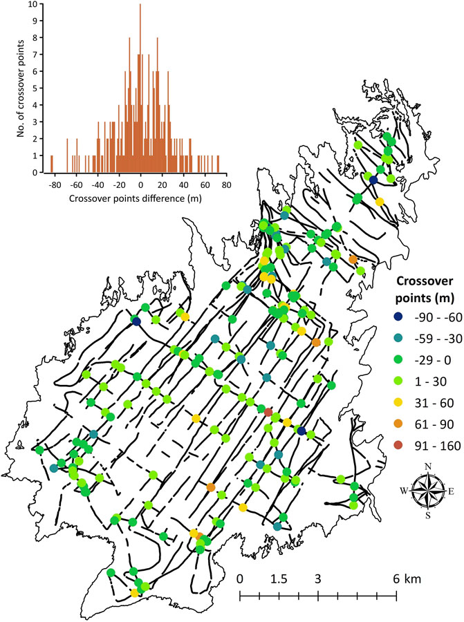
FIGURE 2. Crossover points found between crossing radar profiles (ice thickness, m). Note that the legend range changes at the last two dots. The histogram (upper left corner) shows the distribution of the crossover differences in meters. Most points have a crossover point difference of less than 40 m (the average is 20 m, and the median is 15 m). The black lines illustrate all profiles used for the interpolation of subglacial bed topography.

FIGURE 3

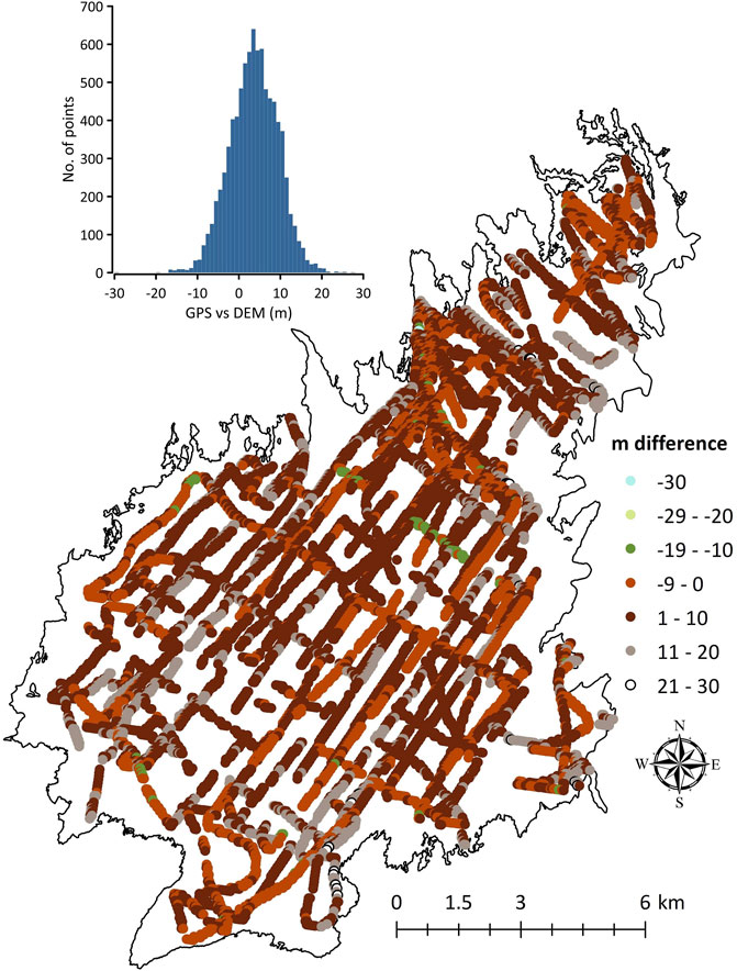
FIGURE 3. The coloured lines illustrate the calculated differences in elevation between the values measured by the ice-penetrating radar GPS and the 2013 DEM (Kartverket/norgeskart.no, 2020). The histogram (top left) shows the distribution of elevation differences. Most of the data have a difference of less than 10 m.

As the elevation accuracy of the radar GPS is difficult to quantify, we compared these measurements to the DEM from 2013 (Kartverket, 2020). The GPS elevation measurements for each radar profile were subtracted from the DEM (Figure 3). The maximum difference is ±30 m, but the difference between most values is within 10 m, and the mean is 5.5 m. There are unavoidable differences between the GPS elevation measurements and the DEM, as the DEM is from 2013 (Kartverket, 2020), and the ice cap has been melting over the past few years (Nesje et al., 2008; Andreassen et al., 2012). As discussed earlier in this section, a 10 m accuracy is within the uncertainty of radar measurements (see the crossover analysis in Figure 2); therefore, both the DEM and GPS data will provide a similar result when used for interpolation and calculation of ice thickness. At Sørfonna, an accuracy of ±10 m is important at its edges, where the ice cap is thinner; in the middle part, where the ice thickness is between 300 and 600 m, 10 m will not have too much effect on the overall shape of the glacier and the glacial bed. For this reason, we analyse large-scale bedrock features and avoid discussing exact numbers for ice thickness when they are smaller than tens of meters. We also cannot discuss individual outlet glaciers’ specific ice thicknesses, as our dataset does not cover most of the outlet glaciers.

The error sources described in this section may have affected the accuracy of the estimated mean ice thickness and volume. To test this, we compared the ice thickness map made in this study to measurements obtained by NVE and Statkraft using radar between 1964 and 2004 on the northwestern part of Sørfonna (Brekke and Nord, 2008). The comparison shows a similar ice thickness pattern in this area (see Supplementary Appendix S3). Of course, the exact numbers differ somewhat because the ice cap and outlet glaciers have both advanced and retreated in past decades, and on the previous map there are more measurement points on the outlet glaciers but fewer on the actual main body of the glacier.

3.3 Dynamical Ice Flow Modelling

The model is based on the continuation equation for mass conservation and is a combination of the two-dimensional shallow ice flow model developed by Meur and Vincent (2003) and the one-dimensional model described by Oerlemans (2001). The model requires five input parameters: glacial bed elevation, glacier surface elevation, mass balance data, quantification of internal deformation, and subglacial sliding. In this study, the mapped subglacial bed, a glacier surface (Kartverket, 2020), and mass balance data (Andreassen et al., 2012), which are described further in the next section, were used as input data. Internal deformation and subglacial sliding were calculated based on empirical parameters following the method described by Laumann and Nesje (2014). The model has previously been used on the plateau glacier Spørteggbreen in western Norway (Laumann and Nesje, 2014) and on Hardangerjøkulen (Laumann and Nesje, 2017). The model is derived from the model developed by Giesen (2009) which has for example been used on Hardangerjøkulen by Giesen and Oerlemans (2010).

To calculate how climate will affect the ice cap, temperature and precipitation must be transformed into mass balance. A simple degree-day model was used for this purpose, with daily temperature and precipitation in Bergen (65 km west of Folgefonna; Smith-Meyer and Tvede, 1996; Braithwaite, 2011; Figure 1) used as input parameters. Bergen was chosen since meteorological stations located in the immediate proximity to Sørfonna would not be applicable for the whole ice cap due to significant difference in local climate close to the ice cap. The model calculates snow accumulation and melting at different elevations on the ice cap. To calibrate the model, the temperature and precipitation gradients (grt, grP), the melting factors for snow and ice (cs, ci), and a correction factor (corr.) for the distance between Bergen and Sørfonna were used to tune the data. This was done by integrating actual mass balance measurements taken during field surveys (Kjøllmoen, 2014; Kjøllmoen, 2018; Norwegian Water Resources and Energy Directorate, 2019) of the outlet glacier Svelgjabreen (southern part of Sørfonna), for which there are 11 years of continuous measurements (2007–2017), and the outlet glacier Gråfjellsbrea (northern part of Sørfonna), for which there are 10 years of continuous measurements (2003–2012).

Tuning each of the above-mentioned parameters is also partly dependent on the tuning of each parameter separately. However, using mass balance data, it is possible to independently calculate the grt for four of the 11 years. The annual measured mass balance for the outlet glacier Svelgjabreen was positive for the three highest elevations. This means that in those years, only snow (not ice) melted at these locations. On average, the ratio between measured melting at the lowest elevation (1,300 masl.) and at the highest elevation (1,600 masl.) is 1.55 m w.e. Assuming a constant melting factor for snow, cs, this will also be the ratio between degree-days at the same elevations. To find this number, grt is the only unknown, and it is calculated to be –0.62°C (100 m) ⁻¹. With known grt, grP is calculated using measured accumulations over 11 years. The two remaining parameters (cs and ci) are found by comparing the average measured and calculated summer balances. The parameters used for Svelgjabreen in the model are as follows: grt = –0.62 ^oC per 100 m, grP = 8% per 100 m, corr. = 1.00, cs = 0.0041 m w.e. ^oC⁻¹d⁻¹, and ci = 0.0059 m w.e. ^oC⁻¹d⁻¹. The parameters used for Gråfjellsbrea are estimated in the same way as for Svegjabreen, and they are as follows: grt = –0.6°C per 100 m, grP = 9% per 100 m, corr. = 0.65, cs = 0.0044 m w.e. ^oC⁻¹d⁻¹, and ci = 0.0060 m w.e. ^oC⁻¹d⁻¹.

Mass balance measurements from NVE show that the mass balance of Sørfonna has a large gradient from north to south (Østrem et al., 1988). The mass balance at every grid point on Sørfonna is thus calculated as a function of elevation and have a latitudinal “lapse rate”.

The model can be tested by modelling a documented time period that has already passed. The glacial extent of Sørfonna was mapped both in 1959 and 2013 (Smith-Meyer and Tvede, 1996). Therefore, the model was tested using the glacial extent in 1959 as input for the model and running it annually until 2013 using the existing calculated and measured mass balance. A comparison was then made between the modelled output and the measured glacial extent in 2013 to verify the model’s robustness (Figure 4).

FIGURE 4

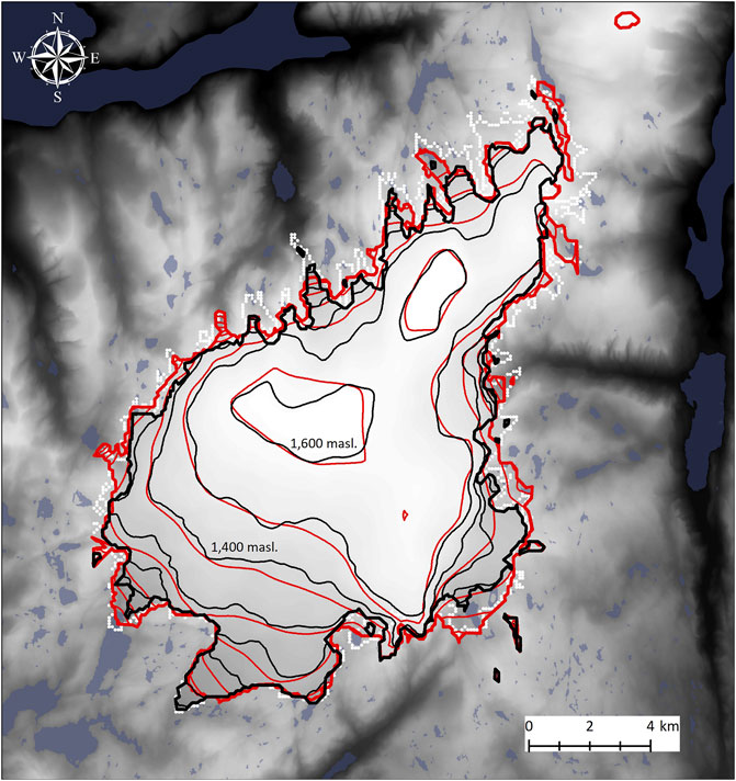
FIGURE 4. Extent of Sørfonna measured in 2013 (black) and modelled extent (red), with the measured glacier extent of 1959 used as the initial input for the model. Area differs 16 km² and, perimeter 6 km, between the two. The white dotted line is the measured extent of the ice cap 1959. The resolution of these extents is 100 m.

3.3.1 Two Climate Scenarios Used to Model the Future Retreat of the Sørfonna Ice Cap

Climate change scenarios from the present day (1971–2000) until the end of the century (2071–2100) are available from the Norwegian Climate Services Centre (Norsk Klimaservicesenter, 2020). In this study, climate scenarios from the county Rogaland, southwest of the Folgefonna peninsula, were used, as these are more representative of precipitation than using scenarios west and north of the glacier. In climate scenario 1, an optimistic scenario, the temperature increases linearly until 2045, when the temperature becomes 1.5°C above current temperatures (1971–2000). From 2045 to 2170, the temperature is kept constant at the 2045 level. An increase in precipitation of 3% was chosen based on predictions of increased precipitation along the west coast of Norway (Lundstad et al., 2018). Climate scenario 2 follows the same trajectory but features a higher rise in temperature and precipitation. This projection is based on continuous growth in greenhouse gas emissions and is often called ‘business as usual’, as no climate measures are implemented. We assumed that the area around Sørfonna will be 3.5°C warmer and will receive 15% more rainfall towards the end of the century compared to today, in accordance with the Norwegian Climate Service Centre (Norsk Klimaservicesenter, 2020). Climate scenario 1 is similar to RCP 2.6 and climate scenario 2 is similar to RCP 8.5.

The mass balance model calculates the average annual mass balance at four elevations for the thirty-year period from 1971 to 2000 using daily precipitation and temperature measurements in Bergen (Florida station, 12 masl.). Similarly, the mass balance from 2071 to 2100 was found for the two scenarios by increasing temperature and precipitation. The results are shown in Table 1. Both scenarios were run until 2170, with a constant mass balance from 2085. Drainage catchment changes were also analysed for every tenth year in the modelled dataset. Changes in drainage pattern due to hydropower production were not considered.

TABLE 1

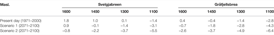
TABLE 1. Calculated annual mass balance (m w.eq.) for Svelgjabreen glacier and Gråfjellsbrea glacier at three altitude levels during the 30-year period 1971–2000 for climate scenarios 1 and 2.

4 Results

4.1 Ice-Penetrating Radar Profiles and Subglacial Topography

The radar profiles (Figure 5) used in the interpolation process of Sørfonna cover the ice cap in a grid with line spacing of approximately 500 $\times$ 1,000 m, as seen in Figure 5A. The middle part, where we began each day in the field (from Fonnabu; Figure 1), features denser line spacing. Some lines are discontinuous in the southern part, making this area slightly less surveyed. As the example profile illustrates (Figures 5B,C), the subglacial topography is far from flat and fluctuates from valleys to mountain peaks. The measurements show that the ice cap is thickest in the south-central part, reaching about 200–600 m, and thins towards the edges as the outlet glaciers flow down into valleys (Figure 6). The northern part of the ice cap is generally thinner, similar to Nordfonna, but it still reaches an ice thickness of more than 300 m in the central parts (Figure 6).

FIGURE 5

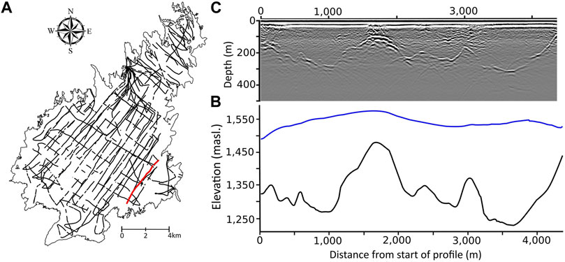
FIGURE 5. (A) Ice thickness profiles used for the interpolation of ice thickness and subglacial bed topography. (B) One radar profile displayed as a graph of the interpreted subglacial bed topography (black line) and glacial ice surface (blue line; masl.). (C) The processed radar profile used for (B). The profiles in B and C are marked as a red line in (A).

FIGURE 6

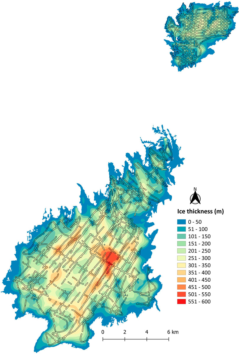
FIGURE 6. Ice thickness calculated by subtracting the interpolated subglacial topography map from the 2013 glacial surface DEM (Kartverket, 2020). Within the black lines is the calculated ice thickness of all measured points used for the interpolation of subglacial bed topography.

The results of the two ice thickness maps (interpolated versus subtracted from DEM) were similar (mean difference = –3 m, standard deviation = 22 m; see figure in Supplementary Appendix S4). The ice thickness map presented in Figure 6 is derived using the DEM surface (see Section 3.1). The maximum measured ice thickness is 568 ± 20 m, the mean ice thickness of the ice cap is 188 ± 20 m, and the volume of the ice cap is 28 km³. Uncertainties are reviewed further in the discussion section.

The interpolated bed topography of both Nordfonna and Sørfonna shows that the smooth dome-shaped glacier surface covers a landscape with deep valleys, hanging valleys, cirques, and glacial over-deepenings, similar to the landscape surrounding the ice cap (Figure 1). The subglacial landscape of Sørfonna has two main valleys draining towards the southwest, with valley floors at 700–800 masl. North, east, and west of these valleys are subglacial mountain peak areas with peaks between 1,200 and 1,500 masl. (Figure 7), resulting in ice thicknesses of less than 50 m in the central parts of the southern dome (Figure 6). There are several high-elevation areas (> 1,400 masl.) in the northern part of the subglacial landscape that are incised by valleys (800–900 masl.) oriented towards the southeast and the northwest (Figure 7). Some valleys and over-deepenings in the landscape are naturally surrounded by water divides and thus may be the locations of lakes in the future. When the ice cap has completely melted and the landscape is ice free, the hydrological analysis suggests that up to thirty new lakes of different sizes will be formed. The largest lake will have an area of 4.7 km² and a volume of 0.28 km³ (Figure 7; Table 2). A future ice-free landscape, including future lakes, of both Sørfonna and Nordfonna is presented in Figure 7. The subglacial landscape of Nordfonna is based on the dataset from Førre (2012) but interpolated using the approach described in Supplementary Appendix S2.

FIGURE 7

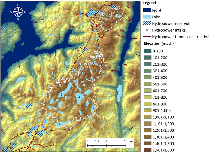
FIGURE 7. Subglacial bed topography and future possible lakes (light blue). Hydropower constructions are marked in red and current reservoir lakes are marked with dark blue stripes. The elevation above sea level is marked by color. The five largest future forming lakes of the Sørfonna landscape are marked by a number (see their parameters in Table 2).

TABLE 2

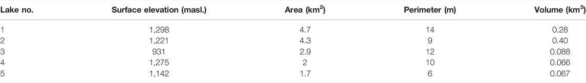
TABLE 2. Attributes (area, volume and perimeter) for the five largest future forming lakes in the landscape currently covered by Sørfonna ice cap (see the lakes in Figure 7).

4.2 Modelling Results: The Future of Sørfonna

Figure 8 shows the modelled Sørfonna ice cap for the years 2120 and 2170, as well as drainage catchments and lakes. Under climate scenario 1, a large part of the 164 km² ice cap is still present in 2120 (101 km²) and in 2170 (76 km²). Under scenario 2, the ice cap is very small (31 km²) in 2120 and likely to be completely melted by 2170 (Table 3).

FIGURE 8

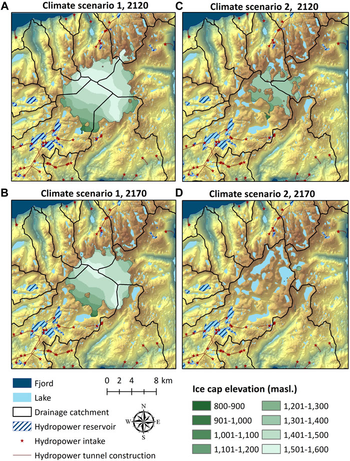
FIGURE 8. (A,B) Model results implementing climate scenario 1 (1.5°C increase), 100 and 150 years in the future. The northern part of the glacier is sensitive and retreats before 2120, but the southern part of the glacier is more resilient. (C,D) Model results implementing climate scenario 2 (3.5°C increase), 100 and 150 years in the future. The glacier retreats faster than in scenario 1. However, even when most of the ice cap is gone in 2120, the drainage basins still have northerly and southerly drainage.

TABLE 3

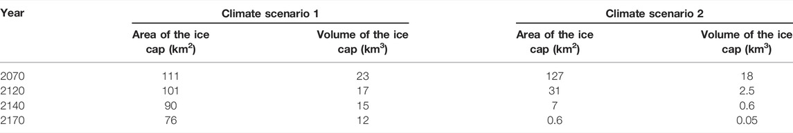
TABLE 3. Decreasing glacial extent and volume of the Sørfonna ice cap for 4 years during climate scenarios 1 and 2.

Using the 1959 extent as input for the model (Figure 4), we successfully reproduced the glacial extent in 2013. Some of the outlet glaciers are not at their full size, and some are larger compared to the DEM measured in 2013 (Kartverket, 2020), but the ice body and the elevation contours of the ice cap concur with the measured and calculated glacial size from 2013. Running the model for the two climate scenarios showed that the southern part of Sørfonna is relatively stable, while the northern part of Sørfonna melts away more quickly (Figure 8).

The present drainage system of the landscape where Sørfonna lies is divided between three major drainage catchments and seven smaller ones (Figure 1). These shift in size when the ice cap melts and therefore altering drainage divides defined by the ice cap. In both climate scenarios, the southwestern drainage catchment, which includes the two major subglacial valleys in the southern part of the glacier, will increase in size, gaining area from the neighbouring catchments (Figure 9). In climate scenario 1, the southwestern drainage catchment will increase by 8 km² by 2120 and 30 km² by 2170. In climate scenario 2, the southwestern catchment will increase by 36 km² by 2120 and 59 km² by 2170. In the northern part of Sørfonna, the drainage configuration is more stable and will remain more or less unchanged as the ice cap shrinks. This change in catchment size indicates a shift towards a more southerly drainage in this landscape compared to present conditions. For a visualization of changes in the drainage catchments and glacial extent for every tenth year, see Supplementary Appendix S5.

FIGURE 9

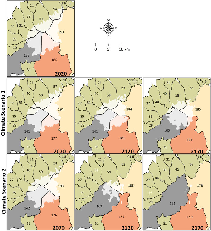
FIGURE 9. Changes in different drainage catchments for three different years in both climate scenarios. The small numbers represent area (in km²) and the white polygon is the modelled extent of the ice cap. The three largest drainage catchments have different colors to make it easier to visualize their change.

5 Discussion

5.1 The Size of Sørfonna and the Glacial Landscape of the Folgefonna Peninsula

The ice thickness map of Sørfonna (Figure 6) shows a maximum ice thickness of above 550 m (the measured maximum depth is ∼570 m), which significantly exceeds the previously measured maximum of 375 m and the estimated maximum of 400 m (Brekke and Nord, 2008; Norwegian Water Resources and Energy Directorate, 2019). Based on our dataset the mean ice thickness is close to 190 m, in contrast with the previous estimate of 140 m (Kennett and Sætrang, 1987; Andreassen et al., 2015). A mean ice thickness of ∼190 m is similar to other ice caps in Norway. For example, the smaller ice cap Hardangerjøkulen (71 km² in area), ∼70 km northeast of Sørfonna, has a mean ice thickness of 150 m and a maximum depth of 380 m (Andreassen et al., 2012). The larger ice cap Jostedalsbreen (474 km² in area), ∼160 km north of Folgefonna, has a mean ice thickness of 160 m and a maximum depth approaching 600 m (Andreassen et al., 2015, and references therein). The previous volume estimate for Sørfonna was 7 km³ (Andreassen et al., 2015), which is lower than Hardangerjøkulen (11 km³) and Jostedalsbreen (49 km³). The calculated volume of close to 30 km³ for Sørfonna presented here is a reasonable volume for an ice cap with the observed area and ice thickness.

This study, combined with the results from Nordfonna (Førre, 2012), shows that the Folgefonna ice cap covers a complex landscape, with deep valleys, hanging valleys, cirques, mountain ridges, and over-deepenings. Qualitative analyses of the subglacial topography below Sørfonna reveal a general consistency with Nordfonna subglacial topography and the landscape surrounding the ice caps. The main valleys of the Sørfonna subglacial topography follow a southwest-northeast direction, lining up with structural weakness zones in the Hardangerfjorden area (Fossen and Hurich, 2005).

5.2 Past and Future Meltwater Draining From Sørfonna

The extent and thickness of ice caps controls the routing of meltwater into surrounding valleys and proglacial and distal glacier-fed lakes. It is therefore possible to constrain bedrock thresholds identified on the subglacial topography map based on numerous existing records of lake sediments surrounding Sørfonna (Figure 10). On the west side of the ice cap, in the valley Bondhusdalen (below Bondhusbreen; Figures 1, 10), radiocarbon ages were reported for the distal glacier-fed Lake Bondhusvatnet (Figure 10) based on a 2.5 m long sediment core (Simonsen, 1999). The uppermost 2 m of the core contains inorganic, partly laminated sediments with low organic content, indicating that the sedimentation is dominated by silt and clay eroded by the ice cap. The lowermost 50 cm of the core contains a high level of organic sediments with high loss-on-ignition values (> 70%). This stratigraphy indicates that there was no input of glacier meltwater into the lake prior to 2240 ± 40 cal yr BP, and that this marks the time when Lake Bondhusvatnet first became a lake in response to the increased input of meltwater from the ice cap (Simonsen, 1999). This is later than the first regrowth of Sørfonna after the Holocene Thermal Maximum (HTM), at ca. 6,900 cal yr BP, which was recorded in Lake Buervatnet (Figure 10) on the eastern side of Sørfonna (Røthe et al., 2019). The subglacial topography map of Sørfonna confirms a threshold below Bondhusbreen, which potentially will redirect its meltwater from the high mountains, from north to south, when the glacier has retreated behind the threshold. Exactly when this will happen can be determined from denser measurements of ice thickness along the threshold, followed by more accurate ice flow modelling in this area, combined with down-scaled climate predictions based on earth system modelling.

FIGURE 10

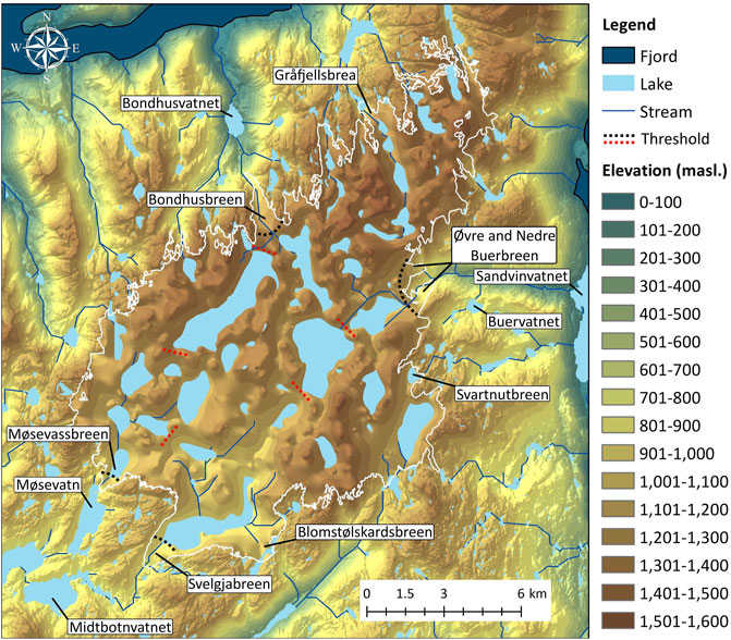
FIGURE 10. The subglacial terrain of Sørfonna with the current (2013) glacial boundary marked as a white line. Thresholds discussed in Section 5.4 are shown as dotted black lines. Dotted red lines show a few of the thresholds that potentially could play a role in a future GLOF event. The names on the map refer to present outlet glaciers and lakes.

On the east side of Sørfonna, two outlet glaciers (Øvre and Nedre Buerbreen; Figures 1, 10) drain towards the distal glacier-fed Lake Sandvinvatnet (Figure 10). The mapped subglacial topography shows a bedrock threshold in the upper part of Buerbreen with an over-deepening to the southwest, which will likely be filled with water when the glacier retreats (Figure 10). Analysis of the sedimentology in Sandvinvatnet indicates that the first glacially derived sediments entered the lake around 4,800 cal yr BP (Ekblom Johansson et al., 2020). Before 4,800 cal yr BP, only organic sediments were present, indicating no glacier in this sub-catchment. Three short recurring periods (2200–1900, 4,600–4,400, and 4,800–4,100 cal yr BP) also show only organic material, which strengthens the theory of a threshold below the outlet glaciers. This is confirmed by observations in the field, where exposed bedrock is visible in the icefall (see image in Supplementary Appendix S6). The glacial return at 4,800 cal yr BP occurred later than for many other glaciers in Norway and differs both from the returns of similar dates at Nordfonna (Bakke et al., 2005) and from glacial reconstruction from the nearby Lake Buervatnet (Røthe et al., 2019). Naturally, glacier growth in the region currently covered by Folgefonna would have begun as isolated patches of ice in high-elevation areas that in time grew to become larger and lower glaciers that eventually merged into the ice cap we see today. Therefore, different glacial return dates after the HTM are possible around the boundary of the present ice cap.

In the southwestern corner of Sørfonna, there is an outlet glacier (Møsevassbreen; Figures 1, 10) with a calving terminus leading into Lake Møsevatn (Figure 10). Reconstruction of former ELA variations based on a study of the sediments deposited in this lake shows a remarkable drop in ELA from 1446 to 1300 cal yr BP, which led to considerable glacier growth (Bjønnes, 2006). After the readvancement of Møsevassbreen, the glacier has been continuously present in the lake catchment. The first part of the record, which covers the past 7,000 years, indicates that no glacier meltwater drained into the lake. This confirms our interpretation of the subglacial topography map; we argue that there is a threshold in the upper part of Møsevassbreen that will direct meltwater from the mountains in an easterly direction when the glacier is smaller than it is today. Inorganic sediment layers from the lake could indicate smaller glacier events from 6,612 to 5,791 cal yr BP, 4,722–4,181 cal yr BP, and 3,000–2900 cal yr BP (Bjønnes, 2006).

A similar study (Wittmeier, 2010) was conducted down-valley from the outlet glacier Svelgjabreen (also called western Blomsterskardsbreen in some studies; Figures 1, 10) based on sediment cores from Lake Midtbotnvatnet (Figure 10). By studying the sediments deposited in this lake, the authors concluded that glacial clay and silt had been continuously deposited from the earliest date (6,295 ± 115 cal yr BP) until the present (Wittmeier, 2010). Their results confirm that the valley below Svelgjabreen drains meltwater from the thickest part of the Sørfonna ice cap. However, it is not possible to conclude whether the glacier was melted completely during the HTM. This contrasts with the work of Nesje et al. (2008) and Bakke et al. (2005), who conclude that all studied glaciers in Norway melted away during the early- and mid-Holocene and regrew during the mid- and late-Holocene.

5.3 Comparison With Other Ice Flow Modelling Studies

By simulating the evolution of Hardangerjøkulen (the closest other ice cap to Folgefonna) from the mid-Holocene to the present, Åkesson et al. (2017) found that Hardangerjøkulen is highly sensitive to climate change. With a projected future warming of 3°C, the model indicates that the Hardangerjøkulen ice cap will disappear almost entirely before the end of the 21^st century, and that not even an improbable 100% increase in precipitation can compensate for the effect of the warming (Giesen and Oerlemans, 2010).

In southern Norway, other glacier model simulations have been carried out using one-dimensional models of Spørteggbreen (Laumann and Nesje, 2014); Nigardsbreen, an eastern outlet glacier of the Jostedalsbreen ice cap (Oerlemans, 1997); Briksdalsbreen, a western outlet glacier of the Jostedalsbreen ice cap (Laumann and Nesje, 2009a; Laumann and Nesje, 2009b); and Storbreen glacier in Jotunheimen (Andreassen and Oerlemans, 2009). Similar to the results from Hardangerjøkulen, sensitivity experiments at Spørteggbreen for a model run from 2011 to 2100 show that an increase in winter precipitation of about 70% is needed to compensate for a warming of 2.3°C (Laumann and Nesje, 2014). The results from Sørfonna presented here show that, at least in the central and southern parts, the ice cap is more resistant to climate change than Nordfonna and other glaciers in western Norway. Runs of the scenario 2 model in our study indicate some ice remnants in 2120, and in scenario 1, there is still ice at Sørfonna in 2170 (Figure 8). Given a present ice volume of 28 km³ (Table 3), Sørfonna has an estimated loss of 43% (17 km³) and 92% (2.5 km³) in climate scenarios 1 and 2, respectively.

Simulations conducted with the Global Glacier Evolution Model (GloGEM)—forced by RCP 2.6 (similar to our climate scenario 1), RCP 4.5, and RCP 8.5 (similar to our climate scenario 2) emission scenarios–yield a global glacier volume loss of between 25 and 48% from 2010 to 2100 (Huss and Hock, 2015). The RCP 4.5 scenario indicates glacier volume losses of 20% in the Arctic, Antarctic, and Subantarctic regions, and 90% in low-latitude regions such as Central Europe (Huss and Hock, 2015). When the evolution of twenty-nine glaciers on Svalbard is modelled under the RCP 8.5 scenario and extrapolated to all land-terminating glaciers on Svalbard, Möller et al. (2016) projections suggest that 1435 ± 59 of the 1471 land-terminating glaciers on Svalbard will be lost by 2100, indicating that it is possible that all the glaciers could disappear. The projected overall volume loss, however, only ranges between 55 ± 36% and 58 ± 37%, due to the nonlinear relation between glaciated areas and ice volumes (Möller et al., 2016). Other studies indicate larger volume losses of the Svalbard glaciers by 2100. For example, Marzeion et al. (2012) project a reduction of 70–84% using RCP 8.5 forcing, and Radić et al. (2014) estimate a reduction of 79–95% following an RCP 8.5 scenario to 2100.

In sum, these results indicate that glaciers with a hypsometry containing small areas above the ELA, such as Spørteggbreen, and thinner ice caps, such as Hardangerjøkulen, are more sensitive to future climate change than Sørfonna. Both the thick ice and the strong precipitation gradient, with more winter precipitation in the south (about 5,000 mm) compared to north (about 3,350 mm), may explain the robustness of the southern part of Sørfonna compared to its thinner and more climate-sensitive northern part. The high amount of winter precipitation may also explain why Sørfonna is likely to evolve more similarly to glaciers at higher latitudes, such as those on Svalbard, and to show more resilience to future warming than other glaciers in southern Norway and Central Europe.

5.4 The Future of Folgefonna: Consequences for Hydropower Production, Tourism, and Geohazards

This study presents the results of an ice flow model based on two scenarios, both of which involve linear forcing and anticipate a gradual rise in temperatures. Despite their simplicity, the model scenarios provide a decent foundation for strategies to adapt to a future with no ice present in the landscape, which are needed by both hydropower companies and society, dependent on the infrastructure around the ice cap. However, every model is a simplification of reality, and the results must be discussed with care. The actual retreat rate depends on the climate outcome which will likely be between the two climate scenarios. Nonetheless, the model provides a strong indication of how and when the ice cap retreats over the area.

We suggest that the resilience of the Sørfonna ice cap is due to the increase in precipitation predicted in the near future, which initially compensates for the increase in temperature. Using climate scenario 2, the ice cap is modelled to be even larger in 2070 compared to the same year using climate scenario 1 (Figure 8). When the ice cap shrinks below its ELA, melting rapidly increases because the accumulation area decreases. When the glacier is still present, drainage catchments will keep draining towards both the north and the south. However, in model scenario 2, the ice cap is completely melted by 2170 (Figure 8D), and the drainage is likely to flow southward. It is possible that the ice cap will become dynamically inactive towards the end. Already in 2120, in climate scenario 2, the ice cap might be too thin (20–100 m; Figure 8C) to be considered an active glacier. In this case, the remaining ice could still act as a water divide.

Although the coverage of the ice-penetrating radar dataset is good for the central parts of the glacier, the outlet glaciers are not as well covered. One example is the outlet glacier Bondhusbreen, where Statkraft AS gathers meltwater directly beneath the glacier at 900 masl. (Figure 1). Our subglacial topography map suggests a ridge underneath Bondhusbreen that acts like a water divide and a boundary for two future lakes. The ice thickness dataset from 1964 to 2004 (Brekke and Nord, 2008), as well as the lake sediment data from Lake Bondhusvatnet (Simonsen 1999), also indicate that there is a bedrock threshold in the upper part of Bondhusbreen. However, to be certain about the elevation of the threshold, more data are needed, with a minimum of one profile oriented perpendicularly over the ridge. The height of this ridge is important, as it determines whether the drainage of the large future lake (no. 1 in Figure 7) just south of the ridge will flow north or south, a distinction of major interest to the hydropower company. If there is ice covering the ridge, the ice flow will be oriented towards the north, allowing Statkraft to continue to intake water directly from Bondhusbreen. When the ice cap retreats beyond the threshold, according to our subglacial topography map of Sørfonna, the drainage will flow to the south. Future adaptation strategies might therefore include more tunnels–if the national park allows their construction. For Sunnhordaland Kraftlag AS, which generates hydropower in the southern sector of the glacier, the water supply seems to be less affected, especially because the valley beneath Svelgjabreen drains a huge area of Sørfonna (Figure 1). However, based on the interpreted threshold north of Møsevassbreen, it is likely that the meltwater drainage will stop in this catchment when the glacier retreats beyond the threshold (Figure 10).

For the tourist industry the area around Folgefonna will change as the glacier slowly retreats. Most of the outlet glaciers will disappear within the next century, and only the highest-lying parts of ice will survive. Based on the above discussion of thresholds under the ice, it is likely that Øvre Buerbreen, Nedre Buerbreen, Bondhusbreen, and Møsevassbreen will be the first outlet glaciers to disappear, along with the northern part of the ice cap. Buerbreen and Bondhusbreen are popular tourist attractions, particularly important to the local economy (e.g., food, accommodations, and guide services).

When Folgefonna retreats, it will expose the area around the glacier to new geohazard threats, such as floods and rock falls. The unstable period of landscape readjustment from glacial to nonglacial conditions is known as the paraglacial period and may last from decades to millennia (Ballantyne, 2002). Even in a small, rapidly responding cirque glacier system, Bakke et al. (2009) showed that the sedimentary input into proglacial Lake Kråkenes was still detectable after 90 years. In larger systems such as Folgefonna, the paraglacial period is deemed to last for millennia, with an exponential shift from hazardous GLOFs and unstable slopes to more subtle changes in glacially conditioned sediment availability (Ballantyne, 2002).

Action needs to be taken to monitor geohazards in areas with rapidly changing glaciers. Known areas with ice-dammed lakes near Sørfonna are mapped by NVE and shown in Figure 11. In the future, when a warmer climate leads to a rapid retreat of the outlet glaciers at Sørfonna, GLOFs will represent a potential danger to infrastructure and society, and the potential locations of GLOFs will shift with the glacier as it retreats. The glacial extent in 2070, shown in Figure 11, would not allow for GLOFs at Buerbreen, as the glacier is beyond the threshold. Just west of Bondhusbreen, however, where historical observations confirm that GLOFs occurred previously (Figure 11), the retreat of the ice cap will form small glacier-dammed lakes in both scenarios 1 and 2, which may cause potential hazards for the heavily touristed areas down-valley in Bondhusdalen. The retreat of Møsevassbreen (Figure 11) might also cause GLOFs when the glacier retreats up the mountain and crosses two new lakes, potentially creating unstable glacier damming. The retreat of Svelgjabreen may create GLOFs in three ways: glacier damming by the main or lateral valley due to asynchronous retreat, ice fall from calving fronts in some of the new lakes, and ice damming of lateral valleys caused by avalanches from steep slopes in the main local valley. The model experiment conducted in this study does not allow for detailed analyses of every outlet glacier, but based on our subglacial topography map, some areas need more attention and, possibly, regular monitoring in the future. See Figure 10 for the subglacial terrain of Sørfonna together with Sørfonna’s current glacial extent (2013) and the outlet glaciers discussed in this section.

FIGURE 11

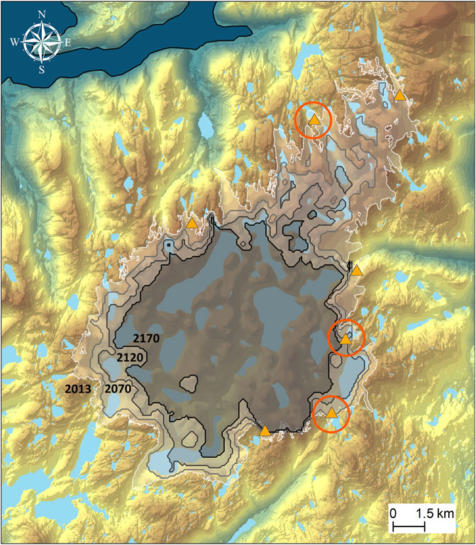
FIGURE 11. The interpolated subglacial landscape of Sørfonna is overlain by today’s glacial extent (white/transparent; 2013) to identify possible locations of GLOFs. The orange triangles represent locations where a GLOF has occurred or where a GLOF is likely to occur, according to NVE. The orange circles mark current GLOF-marked sites with an over-deepening behind the present (2013) glacial margin. The different shades of gray represent the ice cap under climate scenario 1 for the years 2070, 2120, and 2170. Notice the locations of overdeepenings (possible future lake location) where a future GLOF-site could appear.

6 Conclusion

The ice thickness of Folgefonna was determined using a low-frequency radar system, and the datasets were used to interpolate a map over the subglacial terrain beneath Sørfonna and Nordfonna. The results show that the Sørfonna ice cap is thicker than previously estimated and thicker than the Nordfonna ice cap. The subglacial bed topography of Folgefonna resembles the landscape surrounding the present ice caps, with deep valleys and high peaks that are far more irregular than previously described. The subglacial topography reveals thresholds below several outlet glaciers. The mean ice thickness of Sørfonna is calculated to be close to 190 m, and the maximum measured ice thickness is ∼570 m.

We applied a dynamical ice flow model forced by two different climate scenarios to assess the future of the Sørfonna ice cap towards the year 2170. The southern part of Sørfonna shows resilience in a warmer climate, likely due to the high hypsometry and the expected increase in winter precipitation in an already very maritime setting. Compared with other glaciers studied in Norway and other parts of the Arctic, southern Sørfonna seems more resistant to climate change than glaciers at the same latitude, indicating that the maritime climate is favourable for maintaining the ice cap. However, the northern part of Sørfonna is comparable to, for example, Hardangerjøkulen ice cap which is predicted to melt at a faster rate than southern Sørfonna.

We have investigated potential hydrological changes as the glacier melts in a future warmer climate. The map of the subglacial terrain was used to produce a map of future lakes on the Folgefonna peninsula and to analyse changes in drainage catchments during glacial retreat. Future ice loss will cause the main water drainage to shift towards the south when the southern catchments increase in size by gaining area from neighbouring catchments. Subglacial over-deepenings will form up to thirty new lakes of various sizes when the ice retreats. The largest lake will have an area of 4.7 km² and a volume of 0.28 km³. We have also constrained suspected bedrock thresholds by examining previous studies of lake sediment deposited in distal glacier-fed lakes around Sørfonna. Combining this sedimentological evidence with the new subglacial topography map confirms that the retreat of some outlet glaciers, such as Bondhusbreen, Buerbreen, and Møsevassbreen, will have a huge impact on meltwater routing.

Finally, we briefly discussed a few of the many potential areas that will be exposed for increased risk of geohazards. GLOFs are a potential geohazard around Sørfonna, both currently and in the future as the ice cap retreats and new lakes emerge along the glacial margin. There will be need for better monitoring of glaciated areas in a future warmer climate to avoid loss of life and infrastructure.

Data Availability Statement

The raw data supporting the conclusions of this article will be made available by the authors, without undue reservation.

Author Contributions

The study was designed by JB, ES, and FEJ. JB, ES, FEJ, and MG planned and did the fieldwork as well as adapted the radar equipment. FEJ processed and analyzed the data as well as wrote the main part of the manuscript. TL did the glacial modelling. All authors supported the writing of this manuscript.

Funding

This study was funded by TRANS-ENERGY.

Conflict of Interest

The author ES is employed by the company COWI AS.

The remaining authors declare that the research was conducted in the absence of any commercial or financial relationships that could be construed as a potential conflict of interest.

Publisher’s Note

All claims expressed in this article are solely those of the authors and do not necessarily represent those of their affiliated organizations, or those of the publisher, the editors and the reviewers. Any product that may be evaluated in this article, or claim that may be made by its manufacturer, is not guaranteed or endorsed by the publisher.

Acknowledgments

Thank you to Folgefonna National Park, Sunnhordaland Kraftlag AS and Statkraft AS as well as the field crew, including Johannes Hardeng, Torgeir Røthe and Eivind Susort. Also, thank you to Laurent Mingo and Henrik Engström for help with the radar equipment and processing tools.

Supplementary Material

The Supplementary Material for this article can be found online at: https://www.frontiersin.org/articles/10.3389/feart.2022.886361/full#supplementary-material

References

Åkesson, H., Nisancioglu, K. H., Giesen, R. H., and Morlighem, M. (2017). Simulating the Evolution of Hardangerjøkulen Ice Cap in Southern Norway since the Mid-holocene and its Sensitivity to Climate Change. Cryosphere 11 (1), 281–302. doi:10.5194/tc-11-281-2017

CrossRef Full Text | Google Scholar

Andreassen, L. M., Winsvold, S. H., Paul, F., and Hausberg, J. E. (2012). Inventory of Norwegian Glaciers. Oslo: Norwegian Water Resources and Energy Directorate NVE. doi:10.1525/mp.2009.26.3.187

CrossRef Full Text | Google Scholar

Andreassen, L. M., Huss, M., Melvold, K., Elvehøy, H., and Winsvold, S. H. (2015). Ice Thickness Measurements and Volume Estimates for Glaciers in Norway. J. Glaciol. 61 (228), 763–775. doi:10.3189/2015JoG14J161

CrossRef Full Text | Google Scholar

Andreassen, L. M., and Oerlemans, J. (2009). Modelling Long‐term Summer and Winter Balances and the Climate Sensitivity of Storbreen, norway. Geogr. Ann. Ser. A, Phys. Geogr. 91 (4), 233–251. doi:10.1111/j.1468-0459.2009.00366.x

CrossRef Full Text | Google Scholar

Annan, A. (2003). Ground Penetrating Radar Principles, Procedure & Applications. Mississauga: Sensors & Software Inc..

Google Scholar

Aune, B. (1993). DNMI Klima Temperaturnormaler 1961-1990. Oslo: DNMI. Available at: https://cms.met.no/site/2/klimaservicesenteret/Klimanormaler/_attachment/10911?_ts=159b2cddfb3 (Accessed June 20, 2020).

Google Scholar

Bajracharya, S. R., and Mool, P. (2009). Glaciers, Glacial Lakes and Glacial Lake Outburst Floods in the Mount Everest Region, Nepal. Ann. Glaciol. 50 (53), 81–86. doi:10.3189/172756410790595895

CrossRef Full Text | Google Scholar

Bakke, J., Lie, Ø., Heegaard, E., Dokken, T., Haug, G. H., Birks, H. H., et al. (2009). Rapid Oceanic and Atmospheric Changes during the Younger Dryas Cold Period. Nat. Geosci. 2, 202–205. doi:10.1038/ngeo439

CrossRef Full Text | Google Scholar

Bakke, J., Lie, ø., Nesje, A., Dahl, S. O., and Paasche, Ø. (2005). Utilizing Physical Sediment Variability in Glacier-Fed Lakes for Continuous Glacier Reconstructions during the Holocene, Northern Folgefonna, Western Norway. Holocene 15 (2), 161–176. doi:10.1191/0959683605hl797rp

CrossRef Full Text | Google Scholar

Ballantyne, C. K. (2002). Paraglacial Geomorphology. Quat. Sci. Rev. 21 (18-19), 1935. doi:10.1016/S0277-3791(02)00005-7

CrossRef Full Text | Google Scholar

Bjønnes, E. (2006). Rekonstruksjon Av Brefluktuasjonar Og Klimavariasjon På Møsevassbreen , Folgefonna Gjennom Holosen Med Hovudvekt På Neoglasial Tid Og “Den Vesle Istida” (Bergen: Department of Geography, University of Bergen). Master thesis.

Blue Systems Integration Ltd. (2013). IceRadarAnalyzer. 4.1. Vancouver. Available at: http://www.bluesystem.ca/ice-penetrating-radar.html (Accessed May 17, 2017).

Google Scholar

Bradley, R. S., Vuille, M., Diaz, H. F., and Vergara, W. (2006). Threats to Water Supplies in the Tropical Andes. Science 312 (5781), 1755–1756. doi:10.1126/science.1128087

PubMed Abstract | CrossRef Full Text | Google Scholar

Braithwaite, R. J. (2011). “Degree-days,” in Encyclopedia of Snow, Ice and Glaciers (Dordrecht: Springer Nature). doi:10.1007/978-90-481-2642-2_104

CrossRef Full Text | Google Scholar

Brekke, N. G., and Nord, S. (2008). Folgefonna Og Fjordbygdene. Bergen: Nord 4, 29.

Google Scholar

Carrivick, J. L., and Tweed, F. S. (2016). A Global Assessment of the Societal Impacts of Glacier Outburst Floods. Glob. Planet. Change 144, 1–16. Elsevier B.V. doi:10.1016/j.gloplacha.2016.07.001

CrossRef Full Text | Google Scholar

Chevallier, P., Pouyaud, B., Suarez, W., and Condom, T. (2011). Climate Change Threats to Environment in the Tropical Andes: Glaciers and Water Resources. Reg. Environ. Change 11 (S1), 179–187. doi:10.1007/s10113-010-0177-6

CrossRef Full Text | Google Scholar

Cook, K. L., Andermann, C., Gimbert, F., Adhikari, B. R., and Hovius, N. (2018). Glacial Lake Outburst Floods as Drivers of Fluvial Erosion in the Himalaya. Science 362, 53–57. doi:10.1126/science.aat4981

PubMed Abstract | CrossRef Full Text | Google Scholar

Cook, S. J., Kougkoulos, I., Edwards, L. A., Dortch, J., and Hoffmann, D. (2016). Glacier Change and Glacial Lake Outburst Flood Risk in the Bolivian Andes. Cryosphere 10, 2399–2413. doi:10.5194/tc-10-2399-2016

CrossRef Full Text | Google Scholar

Ekblom Johansson, F., Bakke, J., Støren, E. N., Paasche, Ø., Engeland, K., and Arnaud, F. (2020). Lake Sediments Reveal Large Variations in Flood Frequency over the Last 6,500 Years in South-Western Norway. Front. Earth Sci. 8 (239), 1–21. doi:10.3389/feart.2020.00239

CrossRef Full Text | Google Scholar

ESRI (2016b). An Overview of the Hydrology Toolset. Available at: https://desktop.arcgis.com/en/arcmap/10.3/tools/spatial-analyst-toolbox/an-overview-of-the-hydrology-tools.htm (Accessed June 02, 2020).

Google Scholar

ESRI (2016a). Topo to Raster. Available at: https://desktop.arcgis.com/en/arcmap/10.3/tools/spatial-analyst-toolbox/topo-to-raster.htm (Accessed June 02, 2020).

Google Scholar

Førland, E. J. (1993). DNMI Klima Nedbornormaler 1961-1990. Oslo: DNMI. Available at: https://cms.met.no/site/2/klimaservicesenteret/Klimanormaler/_attachment/10912?_ts=159b2ce35a5 (Accessed July 02, 2020).

Google Scholar

Førre, E. (2012). Topografi Og Dreneringsretninger under Nordfonna, Folgefonna (Bergen: Department of Earth Science, University of Bergen). Master thesis.

Fossen, H., and Hurich, C. A. (2005). The Hardangerfjord Shear Zone in SW Norway and the North Sea: A Large-Scale Low-Angle Shear Zone in the Caledonian Crust. J. Geol. Soc. 162 (4), 675–687. doi:10.1144/0016-764904-136

CrossRef Full Text | Google Scholar

Giesen, R. H. (2009). The Ice Cap Hardangerjøkulen in the Past, Presentand Future Climate (The Netherlands: Institute for Marine and Atmospheric research Utrecht, Utrecht University). Ph.D. thesis. Available at: http://igitur-archive.library.uu.nl/dissertations/2009-1104-200130/UUindex.html.

Giesen, R. H., and Oerlemans, J. (2010). Response of the Ice Cap Hardangerjøkulen in Southern Norway to the 20th and 21st Century Climates. Cryosphere 4 (2), 191–213. doi:10.5194/tc-4-191-2010

CrossRef Full Text | Google Scholar

Gruber, S., and Ludwig, F. (1996). Application of GPR in Glaciology and Permafrost Prospecting. Technical Report.Rovaniemi, Finland, 1–22.

Google Scholar

Gulev, S. K., Thorne, J. W., Ahn, J., Dentener, F. J., Domingues, C. M., Gerland, S., et al. (2021). “Changing State of the Climate System,” in Climate Change 2021: The Physical Science Basis. Contribution of Working Group I to the Sixth Assessment Report of the Intergovernmental Panel on Climate Change. Editors V. MassonDelmotte, P. Zhai, A. Pirani, S. L. Connors, C. Péan, S. Bergeret al. (Cambridge: Cambridge University Press). In Press.

Google Scholar

Haakensen, N. (1989). Akkumulasjon På Breene I Sør-Norge Vinteren 1988–89. Været Vis. guide til Meteorol. 13, 91.

Google Scholar

Hallegatte, S., Green, C., Nicholls, R. J., and Corfee-Morlot, J. (2013). Future Flood Losses in Major Coastal Cities. Nat. Clim. Change 3, 802–806. doi:10.1038/nclimate1979

CrossRef Full Text | Google Scholar

Hewitt, K. (1982). “Hydrological Aspects of Alpine and High Mountain Areas,” in Proceedings of the Exeter Symposium, July 1982. IAHS Publ. no. 138.

Google Scholar

Hinkel, J., Lincke, D., Vafeidis, A. T., Perrette, M., Nicholls, R. J., Tol, R. S. J., et al. (2014). Coastal Flood Damage and Adaptation Costs under 21st Century Sea-Level Rise. Proc. Natl. Acad. Sci. U.S.A. 111 (9), 3292–3297. doi:10.1073/pnas.1222469111

PubMed Abstract | CrossRef Full Text | Google Scholar

Huss, M., and Hock, R. (2015). A New Model for Global Glacier Change and Sea-Level Rise. Front. Earth Sci. 3, 1–22. doi:10.3389/feart.2015.00054

CrossRef Full Text | Google Scholar

Immerzeel, W. W., van Beek, L. P. H., and Bierkens, M. F. P. (2010). Climate Change Will Affect the Asian Water Towers. Science 328 (5984), 1382–1385. doi:10.1126/science.1183188

PubMed Abstract | CrossRef Full Text | Google Scholar

Jackson, M., and Ragulina, G. (2014). Report No. 83 – 2014 Inventory of Glacier-Related Hazardous Events in Norway. Norway: Majorstua.

Google Scholar

Kartverket (2020). Høydedata. Available at: https://hoydedata.no/LaserInnsyn/ (Accessed November 20, 2019).

Google Scholar

Kaser, G., Großhauser, M., and Marzeion, B. (2010). Contribution Potential of Glaciers to Water Availability in Different Climate Regimes. Proc. Natl. Acad. Sci. U.S.A. 107 (47), 20223–20227. doi:10.1073/pnas.1008162107

PubMed Abstract | CrossRef Full Text | Google Scholar

Kennett, M., and Sætrang, A. C. (1987). Istykkelsesmålinger På Folgefonna. Oppdragsrapport 18-1987. Oslo: Norwegian Water Resources and Energy Directorate NVE.

Google Scholar

Kjøllmoen, B. (2018). NVE Oppdragsrapport Serie A Nr. 2 Glasiologiske Undersøkelser På Søndre Folgefonna 2007-2017. Oslo: Norwegian Water Resources and Energy Directorate NVE.

Google Scholar

Kjøllmoen, B. (2014). NVE Oppdragsrapport Serie A Nr. 9 Glasiologiske Undersøkelser På Folgefonna 2002-2013. Oslo: Norwegian Water Resources and Energy Directorate NVE.

Google Scholar

Laumann, T., and Nesje, A. (2009a). A Simple Method of Simulating the Future Frontal Position of Briksdalsbreen, Western Norway. Holocene 19 (2), 221–228. doi:10.1177/0959683608100566

CrossRef Full Text | Google Scholar

Laumann, T., and Nesje, A. (2014). Spørteggbreen, Western Norway, in the Past, Present and Future: Simulations with a Two-Dimensional Dynamical Glacier Model. Holocene 24 (7), 842–852. doi:10.1177/0959683614530446

CrossRef Full Text | Google Scholar

Laumann, T., and Nesje, A. (2009b). The Impact of Climate Change on Future Frontal Variations of Briksdalsbreen, Western Norway. J. Glaciol. 55 (193), 789–796. doi:10.3189/002214309790152366

CrossRef Full Text | Google Scholar

Laumann, T., and Nesje, A. (2017). Volume–area Scaling Parameterisation of Norwegian Ice Caps: A Comparison of Different Approaches. Holocene 27 (1), 164–171. doi:10.1177/0959683616652712

CrossRef Full Text | Google Scholar

Lindbäck, K., Pettersson, R., Doyle, S. H., Helanow, C., Jansson, P., Kristensen, S. S., et al. (2014). High-resolution Ice Thickness and Bed Topography of a Land-Terminating Section of the Greenland Ice Sheet. Earth Syst. Sci. Data 6 (2), 331–338. doi:10.5194/essd-6-331-2014

CrossRef Full Text | Google Scholar

Lundstad, E., Håvelsrud Andersen, A. S., and Förland, E. J. (2018). Klimarapport for Odda, Ullensvang Og Jondal Temperatur Og Nedbør I Dagens Og Framtidens Klima. Odda. Available at: https://cms.met.no/site/2/klimaservicesenteret/rapporter-og-publikasjoner/_attachment/13607?_ts=1641d2576b5 (Accessed March 10, 2020).

Google Scholar

Magnússon, E., Belart, J., Pálsson, F., Anderson, L., Gunnlaugsson, A., Berthier, E., et al. (2016). The Subglacial Topography of Drangajokull Ice Cap, NW-Iceland, Deduced from Dense RES-Profiling. Jokull 66, 1–26.

Google Scholar

Marzeion, B., Jarosch, A. H., and Hofer, M. (2012). Past and Future Sea-Level Change from the Surface Mass Balance of Glaciers. Cryosphere 6, 1295–1322. doi:10.5194/tc-6-1295-2012

CrossRef Full Text | Google Scholar

Meur, E. L., and Vincent, C. (2003). A two-dimensional shallow ice-flow model of Glacier de Saint-Sorlin, France. J. Glaciol. 49 (167), 527–538. doi:10.3189/172756503781830421

CrossRef Full Text | Google Scholar

Möller, M., Navarro, F., and Martín-Español, A. (2016). Monte Carlo Modelling Projects the Loss of Most Land-Terminating Glaciers on Svalbard in the 21st Century under RCP 8.5 Forcing. Environ. Res. Lett. 11, 094006. doi:10.1088/1748-9326/11/9/094006

CrossRef Full Text | Google Scholar

Nesje, A., Bakke, J., Dahl, S. O., Lie, Ø., and Matthews, J. A. (2008). Norwegian Mountain Glaciers in the Past, Present and Future. Glob. Planet. Change 60 (1–2), 10–27. doi:10.1016/j.gloplacha.2006.08.004

CrossRef Full Text | Google Scholar

Nicholls, R. (2011). Planning for the Impacts of Sea Level Rise. Oceanog. 24 (2), 144–157. doi:10.5670/oceanog.2011.34

CrossRef Full Text | Google Scholar

Norsk Klimaservicesenter (2020). Norsk Klimaservicesenter. Available at: https://klimaservicesenter.no/ (Accessed February 20, 2020).

Google Scholar

Norwegian Water Resources and Energy Directorate (NVE) (2019). Breatlas. Available at: https://gis3.nve.no/link/?link=breatlas (Accessed July 17, 2019).

Google Scholar

Norwegian Water Resources and Energy Directorate (NVE) (2017). Klima, Nå Og I Framtiden. Available at: https://www.nve.no/klima/klima-na-og-i-framtiden/?ref=mainmenu (Accessed July 17, 2019).

Google Scholar

Oerlemans, J. (2001). Glaciers and Climate Change. Rotterdam.

Google Scholar

Oerlemans, J. (1997). A Flowline Model for Nigardsbreen, Norway: Projection of Future Glacier Length Based on Dynamic Calibration with the Historic Record. A. Glaciol. 24, 382–389. doi:10.1017/s0260305500012489

CrossRef Full Text | Google Scholar

Østrem, G., Selvig, K. D., and Tandberg, K. (1988). Atlas over Breer I Sør-Norge. Oslo: Norwegian Water Resources and Energy Directorate NVE.

Google Scholar

Pälli, A., Kohler, J. C., Isaksson, E., Moore, J. C., Pinglot, J. F., Pohjola, V. A., et al. (2002). Spatial and Temporal Variability of Snow Accumulation Using Ground-Penetrating Radar and Ice Cores on a Svalbard Glacier. J. Glaciol. 48 (162), 417–424. doi:10.3189/172756502781831205

CrossRef Full Text | Google Scholar

Pettersson, R. (2003). Cold Surface Layer Thinning on Storglaciären, Sweden, Observed by Repeated Ground Penetrating Radar Surveys. J. Geophys. Res. 108 (F1), 1–9. doi:10.1029/2003JF000024

CrossRef Full Text | Google Scholar

Purdie, H. (2013). Glacier Retreat and Tourism: Insights from New Zealand. Mt. Res. Dev. 33 (4), 463–472. doi:10.1659/mrd-journal-d-12-00073.1

CrossRef Full Text | Google Scholar

Radić, V., Bliss, A., Beedlow, A. C., Hock, R., Miles, E., and Cogley, J. G. (2014). Regional and Global Projections of Twenty-First Century Glacier Mass Changes in Response to Climate Scenarios from Global Climate Models. Clim. Dyn. 42, 37–58. doi:10.1007/s00382-013-1719-7

CrossRef Full Text | Google Scholar

Radić, V., and Hock, R. (2011). Regionally Differentiated Contribution of Mountain Glaciers and Ice Caps to Future Sea-Level Rise. Nat. Geosci. 4 (2), 91–94. doi:10.1038/ngeo1052

CrossRef Full Text | Google Scholar

Rignot, E., Mouginot, J., Larsen, C. F., Gim, Y., and Kirchner, D. (2013). Low-frequency Radar Sounding of Temperate Ice Masses in Southern Alaska. Geophys. Res. Lett. 40, 5399–5405. doi:10.1002/2013GL057452

CrossRef Full Text | Google Scholar

Robin, G. Q., Evans, S., and Bailey, J. T. (1969). Interpretation of Radio Echo Sounding in Polar Ice Sheets. Philos. Trans. R. Soc. A 256, 437–505. doi:10.1098/rsta.1969.0063

CrossRef Full Text | Google Scholar

Røthe, T. O., Bakke, J., and Støren, E. W. N. (2019). Glacier Outburst Floods Reconstructed from Lake Sediments and Their Implications for Holocene Variations of the Plateau Glacier Folgefonna in Western Norway. Boreas 48 (3), 616–634. doi:10.1111/bor.12388

CrossRef Full Text | Google Scholar

Sandmeier, K. (2016). Reflexw. 8.1. Karlsruhe, Germany: Software Manual. Available at: https://www.sandmeier-geo.de/reflexw.html (Accessed April 20, 2020).

Google Scholar

Simonsen, J. R. (1999). Rekonstruksjon av Holocene brevariasjoner for vestre del av Søndre Folgefonna (Bergen: Department of Geography, University of Bergen). Master thesis.

Smith-Meyer, S., and Tvede, A. M. (1996). Rapport 36 - Volumendringer På Søndre Foolgefonna Mellom 1959 Og 1995. Norway: Majorstua.

Google Scholar

Statkraft AS (2020). Vannkraft | Statkraft. Available at: https://www.statkraft.no/var-virksomhet/vannkraft/ (Accessed July 6, 2020).

Google Scholar

Sutherland, D. G. (1984). Modern Glacier Characteristics as a Basis for Inferring Former Climates with Particular Reference to the Loch Lomond Stadial. Quat. Sci. Rev. 3, 291–309. doi:10.1016/0277-3791(84)90010-6

CrossRef Full Text | Google Scholar

Tvede, A. M. (1989). Floods Caused by a Glacier-Dammed Lake at the Folgefonni Ice Cap, Norway. A. Glaciol. 13, 262–264. doi:10.1017/s0260305500008016

CrossRef Full Text | Google Scholar

Vitousek, S., Barnard, P. L., Fletcher, C. H., Frazer, N., Erikson, L., and Storlazzi, C. D. (2017). Doubling of Coastal Flooding Frequency within Decades Due to Sea-Level Rise. Sci. Rep. 7 (1399), 1–9. doi:10.1038/s41598-017-01362-7

PubMed Abstract | CrossRef Full Text | Google Scholar

Waite, A., and Schmidt, S. (1961). Gross Errors in Height Indication from Pulsed Radar Altimeters Operating over Thick Ice or Snow. IRE Int. Conv. Rec. 5, 38–54.

Google Scholar

Wilson, N. J., Flowers, G. E., and Mingo, L. (2013). Comparison of Thermal Structure and Evolution between Neighboring Subarctic Glaciers. J. Geophys. Res. Earth Surf. 118, 1443–1459. doi:10.1002/jgrf.20096

CrossRef Full Text | Google Scholar

Wittmeier, H. (2010). Glacier Fluctuations and Sediment Transport at Vestre Blomsterskardsbreen, Folgefonna (Bergen: Department of Geography, University of Bergen). Master thesis.

Woodward, J., and Burke, M. J. (2007). Applications of GPR to Glacial and Frozen Materials. J. Environ. Eng. Geophys. 12 (1), 69–85. doi:10.2113/JEEG12.1.69

CrossRef Full Text | Google Scholar

Yde, J. C., Gillespie, M. K., Løland, R., Ruud, H., Mernild, S. H., Villiers, S. D., et al. (2014). Volume Measurements of Mittivakkat Gletscher, Southeast Greenland. J. Glaciol. 60 (224), 1199–1207. doi:10.3189/2014JoG14J047

CrossRef Full Text | Google Scholar

Zemp, M., Huss, M., Thibert, E., Eckert, N., McNabb, R., Huber, J., et al. (2019). Global Glacier Mass Changes and Their Contributions to Sea-Level Rise from 1961 to 2016. Nature 568 (7752), 382–386. doi:10.1038/s41586-019-1071-0

PubMed Abstract | CrossRef Full Text | Google Scholar