Rapid Model Development for GSFLOW With Python and pyGSFLOW

Introduction

Water resources are dynamic and managing them, given competing demands as supplies of both surface water and groundwater change rapidly, is difficult. The challenges are compounded as human reliance on groundwater grows faster than the ability to monitor groundwater supplies (Konikow and Kendy, 2005; Wada et al., 2010). With this background as context, integrated hydrologic models such as GSFLOW (Markstrom et al., 2008) can be used to evaluate management strategies. Integrated models that can simulate surface water and groundwater have potential to improve decision making. However, their benefits are often not fully realized, due in part to errors in model predictions caused by data limitations and incomplete process understanding (Beven, 2019; Blöschl et al., 2019).

Model calibration and application requires hypothesis testing to better represent important processes impacting water storage and flow in hydrologic systems (Clark et al., 2011). Hypothesis testing necessitates rapid processing and construction of input data for multiple models to integrate soft knowledge, test multiple parameter sets, and different conceptualizations; without automation, developing such hydrologic models for river basins is onerous. Automated data processing tools can improve the value of hydrologic models because they reduce the occurrence of data input errors, improve reproducibility, and reduce model construction time and effort (Gardner et al., 2018; Ng et al., 2018).

Techniques for developing and applying coupled surface-water and groundwater models to represent conditions within hydrologic systems have developed along with the design and complexity of hydrologic simulators. In recent decades, hydrologic models have been developed over much larger regions, including river basins (Schoups et al., 2005; Werner et al., 2006; Huntington and Niswonger, 2012; Kitlasten et al., 2021) and continental scales (Wood et al., 1997; Condon and Maxwell, 2015; Regan et al., 2019; Shin et al., 2019). Regional to continental scale models require processing of massive geographic data sets to provide realistic representation of distributed drainage networks. Furthermore, simulating surface-water and groundwater interactions require hydraulic gradients which are sensitive to the relative positioning of streams and topographic features like river canyons, flood plains, and riparian forests (Gardner et al., 2018; Leaf et al., 2021).

Models constructed at river basin and larger scales require sampling digital elevation models (DEMs) at the model grid scale to represent topography. Surface-water networks should be consistent with the both the DEM used to represent the model surface boundary and the model grid scale. Stream networks generated from fine-scale DEMs and overlayed onto coarse DEMs can cause streams to become incongruent, for example streams that are offset from river canyons or unaligned with watershed boundaries. These types of scale mismatches can lead to erroneous surface-water and groundwater exchanges (e.g., reversed hydrologic gradients between surface-water and groundwater systems) and numerical problems (Kampf and Burges, 2007; Schoups et al., 2010; Gardner et al., 2018). Consequently, stream networks often need to be developed consistent with the model surface discretization. Existing software used to build input data sets for large scale hydrologic models have most often relied on stream hydrography data sets built on DEMs at their native scale (e.g., 30 m or finer; Ng et al., 2018; Leaf et al., 2021).

In contrast to using established national stream networks like NHDPlus (Buto and Anderson, 2020), topographic analysis can be used to develop stream networks using DEMs at any resolution. These analyses rely on two geographic data sets used exclusively to develop drainage networks: flow direction and contributing area, also called flow accumulation (O’Callaghan and Mark, 1984; Jenson and Domingue, 1988; Mark, 1988; Tarboton, 1997). Flow direction methods typically choose 1 of 8 possible outflow directions for each grid cell, including directions perpendicular and diagonal to cell faces (D8; O’Callaghan and Mark, 1984) or by using the direction of greatest slope from triangular facets at the center of each grid cell (D-infinity; Tarboton, 1997). Methods that calculate multiple outflow directions for each grid cell and variable flow partitioning also have been applied to address dispersion (Qin et al., 2007). Flow direction methods are then combined with an algorithm for calculating upslope contributing area (Mark, 1988). These approaches form the basis for the popular Arc-Hydro toolset (Maidment and Morehouse, 2002).

Topographic analysis methods used to develop stream networks from DEMs have their own limitations. Digital artifacts in DEMs related to spatial averaging can misassign a flow network and associated model grid cell altitudes. Increasing DEM resolution can reduce these artifacts (Goodchild, 2011); however, finer-scale data are not always available for a geographic area, and computational costs can require coarse spatial discretization for hydrologic models applied to large regions. In low relief basins, spatial averaging can lead to digitally closed sinks, create uncertainty in flow direction assignment, or even lead to digital flow directions that contradict the natural system. Hydrologic conditioning methods such as digitally filling (Jenson and Domingue, 1988; Garbrecht and Martz, 1997; Metz et al., 2011) and outlet breaching (Martz and Garbrecht, 1999) can be applied to the DEM or flow-direction system to remove sink artifacts from flow accumulation. Uncertainty in flow direction assignment generally occurs in flat areas of DEMs associated with low relief watersheds and create maze-like conditions where flow directions cannot be determined without additional information. Previous approaches to solving digitally flat areas have included iterative methods to connect uncertain flow directions (Jenson and Domingue, 1988), incrementally raising flat portions of a DEM to create a gradient from higher terrain to lower terrain (Garbrecht and Martz, 1997), cost function solutions (Metz et al., 2011), and weighted topological methods (Zhang et al., 2017). Given these issues and solutions, stream networks produced for hydrologic modeling are a simplification of the actual network limited primarily by DEM scale and model scale resolution.

Previous approaches for developing coupled surface-water/groundwater systems that can be simulated with GSFLOW (Markstrom et al., 2008) have relied on multiple software tools. GSFLOW is an integrated hydrologic modeling software that couples surface-water processes from the Precipitation Runoff Modeling System (PRMS; Markstrom et al., 2015) and groundwater processes from MODFLOW (Harbaugh, 2005; Niswonger et al., 2011) and is often applied to build models at scales of 10s to 1,000s of km². GSFlow-ArcPy provides functionality to transform raster data sets, such as a DEM or land use/land cover data sets, into PRMS input files (Gardner et al., 2018). GSFLOW-GRASS allows users to build GSFLOW input files from raster and vector data through a command line scripting process within a GRASS GIS environment (Ng et al., 2018). SFRBuilder (Leaf et al., 2021) overlays vector data of streamlines provided by NHDPlus or another custom hydrography dataset onto a DEM to develop the Streamflow Routing Package (SFR) in MODFLOW. PRMS-Python allows the user to load, modify, and run simulation scenarios with existing PRMS input data sets (Volk and Turner, 2019). Finally, the FloPy Python package allows users to build and modify most MODFLOW package files that represent the groundwater system in GSFLOW (Bakker et al., 2016; Bakker et al., 2022). Although these tools can be used to complement each other and create most of the GSFLOW input, proprietary software is sometimes required and manual edits to input files and additional scripts are needed to build, edit, run models, and process output data. These requirements create a disconnected process which requires multiple tools and/or scripts to develop input files and estimate parameters for the surface-water and groundwater systems and hinders reproducibility.

Based on a need for a rapid, reproducible, and robust GSFLOW model building pipeline, we seek to address the needs of constructing complex stream networks from large geographic data sets by presenting the latest version of pyGSFLOW (pronounced “pie-g-s-flow”). The pyGSFLOW Python scripting library allows users to develop input files and set boundary conditions, climate forcing, and hydrologic parameters, edit existing GSFLOW input files, and postprocess model results (Larsen et al., 2021; 2022). Instead of creating an entirely new approach, pyGSFLOW improves upon previous conceptual frameworks and leverages existing tools to create a framework for constructing GSFLOW models (Henson et al., 2013; Gardner et al., 2018; Larsen et al., 2021; Bakker et al., 2022; Larsen et al., 2022). The pyGSFLOW package leverages FloPy (Bakker et al., 2022) for interfacing with MODFLOW model files and integrates this functionality with custom features for interfacing with PRMS and GSFLOW model files. This work extends the existing pyGSFLOW software (Larsen et al., 2021; 2022) with new open-source methods to construct flow direction, flow accumulation, watershed and subbasin delineation, and stream network data sets. These advancements add robustness to the model development process.

Methods

The approach presented here improves upon the existing pyGSFLOW package (Larsen et al., 2021; 2022) to include model-building tools for rapidly generating GSFLOW (Markstrom et al., 2008) models from external raster data. The pyGSFLOW model building tools are part of an open-source python toolkit and can ingest and process ancillary data sets to produce intermediate and primary data required by GSFLOW. Table 1 provides a list of data sets that are required to build a simple GSFLOW model; additional data not included in this list can be used to modify the model. This process can be started or stopped at any point to allow modifications to pre-existing models or to update a single part of the workflow. The steps are presented in the following sections and an overview describing the required data for each step is outlined in Table 1.

TABLE 1

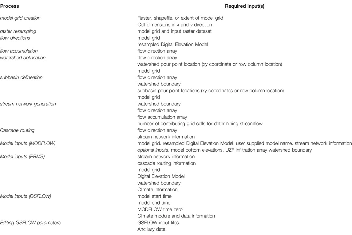
TABLE 1. Overview of the pyGSFLOW process types and the required input data to create a simple GSFLOW model.

Model Grid Creation and Raster Resampling

Model spatial discretization, referred to herein as a model grid, serves as the foundation for building hydrologic models in GSFLOW. GSFLOW and MODFLOW-NWT model grids are structured cellular grids, composed of rectangular cells that are discretized on the basis of row and column spacing. Model grid discretization choices affect not only the location of boundary conditions but also the numerical solution of a model (Markstrom et al., 2008). The pyGSFLOW package provides support for quickly creating rectilinear model grids from geographic information. A raster, shapefile, or bounding box can be supplied with grid spacing information to produce a model grid. Upon creation of the model grid, raster resampling to the model grid scale is accomplished with a simple Python function from FloPy’s “Raster” class (Bakker et al., 2016; Bakker et al., 2022).

The model grid produced by pyGSFLOW is a FloPy “StructuredGrid” (Bakker et al., 2022) object that contains polyline, polygon, and geographic feature information. Resampling the native DEM to the model grid produces an array of raster values consistent in shape and size to the model grid. Model grid land-surface elevations can be calculated for each model grid cell using mean, median, minimum, maximum, or interpolated elevations resampled from the native DEM. The model grid and the resampled DEM are used to develop the flow direction, flow accumulation, and stream network, as described in the next sections.

Flow Direction and Flow Accumulation

Gridded flow-direction calculations determine the direction of flow based on the slopes between a cell and each of its neighboring cells. For 8-direction (D8) flow direction calculations, information for a cell and its 8 adjacent cells are compared (Jenson and Domingue, 1988). Calculations are performed on elevation data resampled from a DEM, and a one-to-one outflow connection is assumed (Jenson and Domingue, 1988). The flow direction is set by calculating the cell index ($i_{cell}$) using Eq. 1.

$i_{cell}=argmax\left(\frac{\mathrm{\Delta }\overrightarrow{e}}{\sqrt{\mathrm{\Delta }{\overrightarrow{x}}^2+\mathrm{\Delta }{\overrightarrow{y}}^2}}\right)(1)$

where $\Delta \overrightarrow{x}$ and $\Delta \overrightarrow{y}$ are the difference between a cell’s center coordinates and a vector of neighboring cell’s center coordinates, and $\Delta \overrightarrow{e}$ is the difference between a cell’s elevation and a vector of its neighbors’ elevations. Once $i_{cell}$ is known, the flow direction is encoded with a digital number that describes the outflow direction using the convention:

$\left[\begin{array}{ccc}64& 128& 1\\ 32& -1& 2\\ 16& 8& 4\end{array}\right]$

where −1 represents the model cell for which calculations are being applied and the digital numbers 1 through 128 represent the specific direction of neighboring cells relative to the model cell. When $i_{cell}$ is not a unique value, flow direction is undefined based on the slope between cells. The pyGSFLOW package’s default method of solving flow direction for undefined cells is a topological method that maps each undefined cell to the nearest outlet and attempts to minimize the absolute distance of the flow direction to the outlet. In cases where the default method does not perform well (e.g., in large, complex, digitally flat areas), a modified version of Dijkstra’s (1959) algorithm can be used to solve the flow direction problem. The pyGSFLOW implementation of Dijkstra’s (1959) algorithm first creates a connectivity graph of all cells and their potential flow paths within a digitally flat area. The algorithm then solves the digitally flat area from the outlet location and minimizes the routing distance for each cell within the graph by weighting each potential flow direction by the routing distance to the outlet. Although hydrologic conditioning is recommended to fill sinks prior to calculating flow directions, a breaching stage threshold can be applied for cases where small digital artifacts in the DEM data create sinks or produce flow directions that conflict with the hydrologic flow system. The breaching stage threshold is a small user defined value that can be used to smooth out differences in resampled DEM elevation values caused by artifacts. Elevation differences between neighboring cells smaller than the breaching stage threshold are considered as equal in elevation which allows the flow direction to pass over a slightly higher cell. The “FlowAccumulation” object in pyGSFLOW performs the flow direction, as well as flow accumulation, calculations from a model grid object and a DEM (shown in “Sagehen Creek Watershed Example” section).

Flow accumulation calculates the number of upslope cells that drain to each cell within the watershed. The flow direction array defines the connectivity of cells and drainage pattern for the flow accumulation calculation. For the D8 flow direction model, each cell can have flow drain into it from multiple neighbors; however, the flow from each cell only can drain to a single neighbor. Flow accumulation numbers are calculated using a queue where accumulation numbers of downstream cells are increased as each cell is taken off the queue, and the number of input drainage paths for the given cell is decreased by one (Wang et al., 2011). If the number of input drainage paths for a cell equals zero, it is added back to the queue. The algorithm completes when the queue is empty.

Watershed and Subbasin Delineation

Watershed boundary delineation is calculated from flow direction arrays following Jenson and Domingue (1988). In-lieu of automated subbasin delineation, user supplied watershed outlets, called “pour points,” are used to define the outlet locations for both the watershed and subbasin delineation calculations. From a single pour point, a topological diagram that includes connection information from the flow direction array is produced, and a watershed is classified from topographic divide information inherent in connection data from the flow direction array. Subbasin delineation is performed in a similar manner as watershed delineation. Multiple pour points are supplied by the user and subbasins, within a watershed, are classified with a unique value. Upstream subbasin boundaries are respected while delineating downstream subbasins. This approach is preferable to fully automated subbasin delineation because hydrologic areas of interest and contributing areas for gaged flows can be isolated by the user for subsequent parameterization, calibration, and output analysis.

Stream Network Generation

Stream network generation is a critical step in defining model boundary conditions for both PRMS and the Streamflow Routing Package (SFR; Niswonger and Prudic, 2005) components of GSFLOW. Streams in GSFLOW are discretized into reaches and segments, where a reach is a part of stream spanning a grid cell, and a segment is generally defined as a stream spanning two confluences or the start of a stream to a confluence. Stream segments can also be further divided at the user discretion to represent other surface-water features such as diversions. Network generation has three distinct parts: classifying grid cells that contain streams, defining the connectivity between stream cells, and defining the number of cells that drain to each stream cell. Stream cell classification is performed by comparing the contributing number of cells in the flow accumulation array data to a user-specified threshold. If the number of accumulated cells is greater than the user-specified threshold value, the cell will be classified as a stream cell. Stream connectivity and flow direction are determined using information from the flow direction array to ensure that streams are continuously connected and that flow occurs in the downslope direction. Clusters of adjacent stream cells are grouped into segments based on the connectivity of the flow direction array. Stream segments either begin at the most upstream cells based on the flow directions or at locations where more than one stream cell drains into a cell. Stream segments end either at a confluence of stream cells, the watershed outlet, or at the watershed boundary. After grouping, topological sorting (Kahn, 1962) and renumbering is performed on the stream network to ensure upstream flows are calculated before downstream flows and to provide optimal calculation order for GSFLOW. Finally, a graph of landscape flow connectivity is created from the flow direction array and stream cells. Each cell is then assigned to a specific stream segment to which it drains.

Once the stream network has been produced, cell to cell routing information for PRMS, referred to as cascade routing, can be extracted from the existing flow direction arrays and the stream network. Because flow direction calculations rely on a D8 method, the cascade routing calculation allows many cells to contribute flow to a single cell, but an individual cell can only drain to 1 cell.

Model Input Generation

PRMS and MODFLOW packages reliant on the stream network can be generated after the stream connectivity has been determined. A set of default model input parameters are stored in a JavaScript Object Notation (JSON) file that can either be loaded, edited by the user, and supplied to the package generation classes or be automatically applied by the package generation classes. These parameters are then passed to their respective PRMS and MODFLOW packages and by default, a single-layer model is created with a GSFLOW control file, PRMS parameter file, and MODFLOW packages (Table 2). After Python input objects are generated, the user can write these inputs to file, edit existing model parameters, and/or add additional information and packages to the model. Because integrated hydrologic modeling includes many more processes than DEM information can provide alone, this approach allows the user to define many additional processes—e.g., vegetative cover, soil zone, climate, pumping, general head boundaries, etc.—outside of the automated model builder methods. Groundwater flow processes can be added or edited with FloPy (Bakker et al., 2016; Bakker et al., 2022), and surface-water water processes including simulation modules can be adjusted with built in functionality from pyGSFLOW (Larsen et al., 2021; 2022). Climate information can be applied as daily time-series information from one or multiple climate stations to the data file or as arrays in climate by hydrologic response unit (grid cell; HRU) files and adjustment factors can be specified in the parameter file. The pyGSFLOW approach gives the user flexibility on how best to represent the climate of the simulated watershed and provides python tools to aid in the processing and writing of these input files. After input objects are generated, users can write the packages to GSFLOW compatible input files and then run the model.

TABLE 2

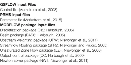
TABLE 2. GSFLOW model input files that are produced with pyGSFLOW’s automated model building methods. Note that climate input files are not automatically populated with default values and instead the user must specify their climate representation.

Editing GSFLOW Model Parameters

After model creation, surface-water and groundwater parameters are commonly added or adjusted in the model calibration process. The pyGSFLOW package allows the user to easily add new parameters, remove unused parameters, and edit existing ones within a python environment. Surface-water parameters, such as land cover, impervious surfaces, and soil physical properties, can be sampled from existing raster data using the raster resampling methods described earlier. Once a raster has been sampled into an array, it can be set directly as a parameter, be scaled or masked, or be used in a mathematical relationship to derive one or multiple parameters. Groundwater parameters can be added and edited using FloPy’s built in features (Bakker et al., 2016; Bakker et al., 2022). After model parameters have been adjusted, new input files can be written for subsequent model runs and analysis. More information and detailed instructions on pyGSFLOW’s usage can be found in Larsen et al. (2021).

Example Problems

Two example problems are presented in this section where the first example illustrates the robustness of pyGSFLOW to develop model input for a complex watershed and the second example demonstrates the utility of pyGSFLOW to rapidly produce multiple conceptualizations of a hydrologic model. The first example is of the Russian River watershed. Only a cursory description is provided for the “Russian River Watershed Example”; instead, the example focuses on demonstrating the robustness of pyGSFLOW for automatically developing a stream network and watershed boundary in a complex watershed. The second example is of the undeveloped Sagehen Creek watershed. This example demonstrates the complete process of building and running the model, including descriptions of all the required ancillary data. The “Sagehen Creek Watershed Example” provides detail to convey each step in the GSFLOW model construction process for a simpler watershed that is computationally inexpensive to build for testing and evaluating results across different users and computing environments.

Russian River Watershed Example

The Russian River watershed, in northwestern California, was chosen as an example to illustrate the stream network generation methods (Figure 1). Construction of the stream network for the Russian River provides an opportunity to showcase pyGSFLOW’s capabilities in a complex system; however, because this system has extensive anthropogenic modifications, it is beyond the scope of this work to present a fully functional model of the Russian River watershed. For this example, only details regarding the grid and stream network generation are provided.

FIGURE 1

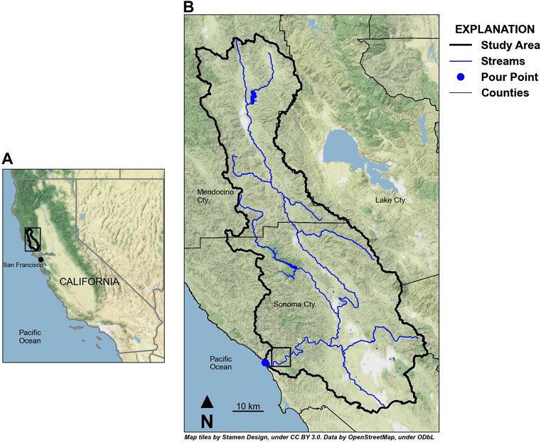
FIGURE 1. Location of the Russian River watershed study area in northwestern California (A). Main drainages of the Russian River watershed provided by NHDPlus dataset (Buto and Anderson, 2020) within the study area boundary (B). Black box inset in (B) defines the boundary for flow direction vectors shown in Figure 3.

The Russian River’s main channel flows from north to south for about 180 km and drains about 3,850 sq. km. of Mendocino and Sonoma Counties to the Pacific Ocean (Figure 1). The watershed contains both steep terrain from the northern coastal range and gentle to flat terrain within the valley regions. Large sections of the watershed are digitally flat at 30 m DEM resolution, parts of the watershed near the Russian River have steep canyon walls with low relief river drainage that creates digital artifacts, and large sections of the watershed have significant topographic relief. The process for generating a flow network for the Russian River watershed begins with DEM selection, spatial discretization, and resampling the DEM to the spatial discretization of the model. A 1 arc-second DEM product was selected for the Russian River watershed (U.S. Geological Survey, 2020). Grid cell size for the Russian River watershed was set to 300 m × 300 m (410 rows, 252 columns; 103,320 grid cells) to adequately represent the topography of the watershed without creating a model that is too computationally demanding. GSFLOW is most often applied to regional-scale systems ranging in size from 10 s to 1,000 s of km² to answer questions about water resources, and the total number of model cells were determined to meet the computational constraints for the project. The DEM was resampled using the minimum elevation in each model grid cell to produce a model-elevation profile that can be used to construct the GSFLOW model (Figure 2).

FIGURE 2

FIGURE 2. Digital elevation model (27.28 m x 27.28 m; DEM; U.S. Geological Survey, 2020) of the Russian River study area (A). DEM values were resampled by minimum elevation to model grid size (300 m × 300 m) and are shown for a subset of the watershed: the raw DEM data (27.8 m resolution) (B) and the resampled DEM values (300 m resolution) (C) correspond to the inset box in (A).

Preparation of the Russian River DEM for flow direction and flow accumulation processes involved filling large sinks and pits prior to resampling to the grid scale (Wang and Liu, 2006). Groups of cells in the model grid that have a lower elevation than their surrounding cells are referred to as sinks that must be filled to provide continuous pathways across all cells from all ridges in the watershed to the watershed outlet at the Pacific Ocean. However, this sink-filling process did not remove all digital artifacts within the watershed. Near the watershed outlet, artifacts from high-relief canyon walls that border low-relief valley floors persisted. In parts of the DEM, large digitally flat areas were also present. Model grid cell elevations adjacent to the Russian River’s outlet, in the Pacific Ocean, were slightly lowered to create a unique condition that Dijkstra’s (1959) algorithm could solve. In the case of a non-unique watershed outlet (all cells are the same elevation), Dijkstra’s algorithm is unable to automatically identify an outlet cell and will try to choose an outlet cell that minimizes the number of uncertain connections, which can yield unexpected results.

Flow direction and flow accumulation processes were applied on the resampled DEM. Flow direction vectors, created from the flow direction array, show that the solution generally follows existing NHDPlus flowlines (Figure 3A). A comparison of the flow direction arrays produced by using pyGSFLOW’s Dijkstra algorithm to solve digitally flat areas (Figure 3A) and pyGSFLOW’s default topographic method shows that 1) the Dijkstra algorithm is well suited to solve this problem and 2) the simple topological method is unable to solve this complex scenario (Figure 3B). Furthermore, a small breaching threshold (1.52e-3 m) was applied to resolve the diverging flow directions caused by digital artifacts. Flow accumulation processes were run to calculate the contributing area to each cell. For the Russian River watershed this process creates an array of values that represent the drainage watershed area for each cell. A threshold of 30 grid cells or about 2.7 km² of contributing area was applied to define the Russian River watershed stream network (Figure 4).

FIGURE 3

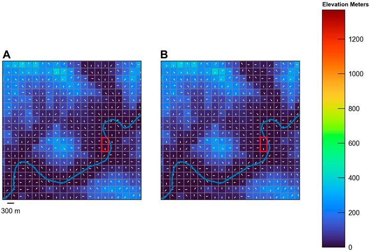
FIGURE 3. Maps showing calculated flow direction vectors for a part of the Russian River watershed (inset box in Figure 1B) with a low relief valley bounded by steep topography. The modified Dijkstra Algorithm (Dijkstra, 1959) produces flow direction vectors that generally follow the NHDPlus streamline (blue; Buto and Anderson, 2020) (A). The red box shows a problem section of the watershed that contains digital artifacts. Stream direction vectors within the red box drain downstream in (A). The red box in (B) shows stream direction vectors that diverge from the watershed drainage pattern and create a condition where the flow direction array does provide a continuous drainage path.

FIGURE 4

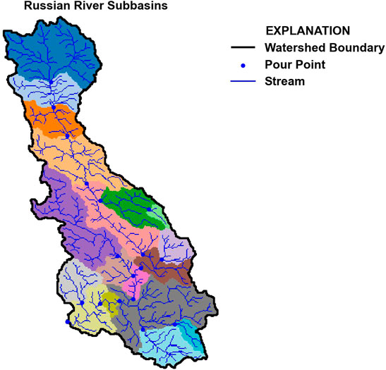
FIGURE 4. Watershed and subbasin delineation results for the Russian River watershed. U.S. Geological Survey streamgages (U.S. Geological Survey, 2021) were supplied to the script as pour points for watershed and subbasin delineation. The black outline represents the Russian River watershed, and unique colors represent individual subbasins calculated by pyGSFLOW. Blue lines show the stream network generated from 1 Arc-second (27.28 m) digital elevation data (U.S. Geological Survey, 2020) by pyGSFLOW, Russian River watershed, northwestern California.

The final steps to prepare the Russian River surface-water network were to define the watershed and subbasin boundaries within the watershed. A single pour point was selected at the outflow location of the Russian River to the Pacific Ocean to define the watershed. The “define_watershed” method in pyGSFLOW (method shown in the “Sagehen Creek Watershed Example”) was applied to the flow direction array to binarize the grid into active and inactive model cells (watershed outline shown in Figure 4). Subbasin delineation was then run. Pour points were selected based on the locations of streamgages throughout the watershed to isolate contributing areas to the streamgages. These contributing areas were grouped using a unique numerical identifier and are presented in Figure 4.

Results from stream generation were compared to the flow accumulation methods available in ArcGIS Pro. Both methods were able to produce representations of the Russian River stream network from the same pour point (Figure 5), and in much of the watershed, both methods follow the same path. Some differences are present in low relief and digitally flat parts the watershed. For example, in the southern part of the Russian River watershed, the ArcGIS Pro stream representation has sections follow a completely straight path, whereas our method produces a sinuous section of stream cells (Figure 5). Both representations of the stream network would likely be suited for hydrologic modeling; however, pyGSFLOW is open-source, and additions and inputs can be suggested by the larger modeling community.

FIGURE 5

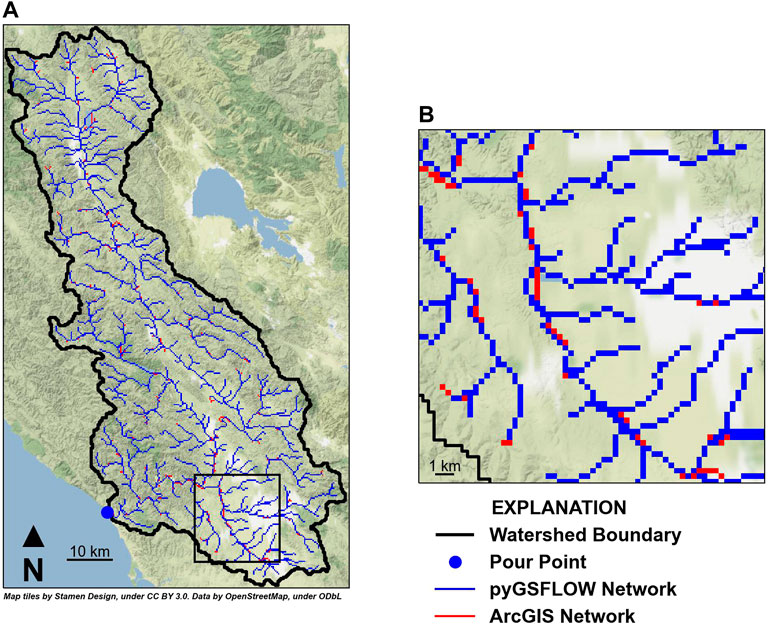
FIGURE 5. Stream network generation from pyGSFLOW (blue lines) and ArcGIS Pro’s Flow Direction and Flow Accumulation tools (red lines) show that both methods are able to create representations of the Russian River watershed’s drainage pattern (A). Some differences in the two stream network representations are observed in low-relief areas throughout the watershed (B).

Sagehen Creek Watershed Example

The Sagehen Creek watershed is located near Lake Tahoe, California, in the northern Sierra Nevada (Figure 6). The watershed drains an area of about 27 km² and has an east facing aspect with about 720 m of relief. The Sagehen Creek watershed has been described in detail and documented as a GSFLOW example problem by Markstrom et al. (2008). In this example, pyGSFLOW model building tools are applied to the Sagehen Creek watershed to create two separate GSFLOW models from raster data with model grid discretization of 50 m × 50 m and 90 m × 90 m to illustrate the utility of pyGSFLOW for creating multiple model frameworks or conceptualizations of the same hydrologic system; specifically, the grid-cell size is evaluated with respect to simulated streamflow and surface-water/groundwater exchanges. This version of the Sagehen Creek watershed model has a different spatial discretization compared to that presented by Markstrom et al., 2008 and consequently has a different set of parameter values and solution.

FIGURE 6

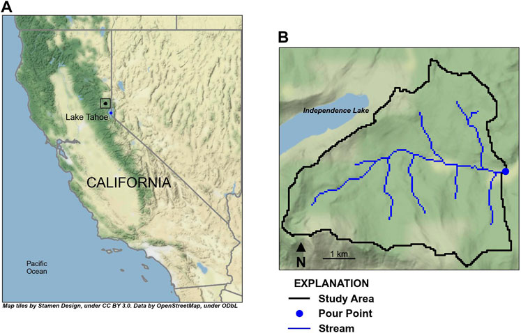
FIGURE 6. Location of the Sagehen Creek watershed study area near Lake Tahoe, California, in the northern Sierra Nevada (A); the study area extent (black outline), Sagehen Creek watershed streamlines (blue lines), and USGS streamgage (10,343,500 SAGEHEN C NR TRUCKEE CA; U.S. Geological Survey, 2021; blue marker) is shown in (B).

Ancillary data sets used to develop the Sagehen Creek GSFLOW model with pyGSFLOW include a 1 arc-second (30 m) resolution DEM for the Sagehen Creek watershed area (U.S. Geological Survey, 2022), a pour point located at the USGS streamgage near the outlet of the watershed (10,343,500 SAGEHEN C NR TRUCKEE CA), LANDFIRE existing vegetation layers (LANDFIRE, 2016), SSURGO 1:24,000 inventory of soil and non-soil layers (USDA, 2021), National Land Cover Database (NLCD) impervious cover data layer (National Land Cover Database, 2020), and PRISM 30-years normals (PRISM Climate Group, 2014). Data from Sagehen Creek co-operative station were provided by University of California, Berkeley (2008), and these daily values of minimum and maximum air temperature and precipitation were distributed to all model grid cells using the PRMS modules temp_1sta and precip_1sta and adjustment factors calculated from the PRISM 30-years normals (800 m resolution), due to spatial resolution constraints from PRISM daily data (4 km resolution).

Two scripts were written specifically for the Sagehen Creek watershed example to construct models with a constant 50 m × 50 m grid cell size (50 m model) and a constant 90 m × 90 m grid cell size (90 m model). These scripts processed the ancillary data sets to construct the GSFLOW models with pyGSFLOW. The outline of the Sagehen Creek watershed script is provided below to illustrate the process. However, some of the coding is not included here for brevity, and users can refer to the two python scripts, Sagehen_50 m py and Sagehen_90 m py or example notebooks, included in the pyGSFLOW repository for details:

1) Generate a structured model grid and resample the native DEM to the model grid:

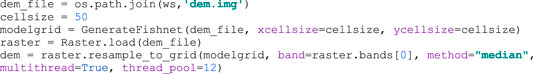
2) Generate the flow direction and flow accumulation data sets for the model grid:

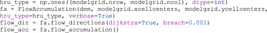
3) Define the watershed boundary using the pour point located at the USGS streamgage:

4) Generate the stream network and cascade directions used to route flow from overland runoff and interflow to streams:

5) Generate the MODFLOW component of the GSFLOW input files using the Fishnet and stream network:

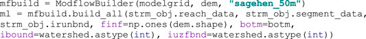
6) Generate the PRMS component of the GSFLOW input files:

In addition to building the MODFLOW and PRMS components, the GSFLOW control and climate data file also must be built using pyGSFLOW, as shown in the Saghen_50 m py script. Because Sagehen Creek has a relatively small watershed, manual calibration was used here by adjusting MODFLOW input data and PRMS parameters using pyGSFLOW. Manual calibration of the Sagehen Creek watershed for the 50 and 90 m models followed a stepwise procedure outlined by Hay et al. (2006). The MODFLOW input data sets and PRMS parameters determined from the calibration of the 50 m model were first directly applied to the 90 m Sagehen Creek watershed model and then calibrated to evaluate the effects of grid cell size on simulated streamflow (Table 3).

TABLE 3

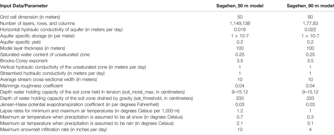
TABLE 3. Parameter values for models using two different spatial resolutions. Parameter values were modified from their default values to calibrate the model with 50 m by 50 m horizontal discretization, and calibrated parameters for the 90 m by 90 m model. Simulated snowpack, temperature, and horizontal hydraulic conductivity values were sensitive to changes in model discretization.

Both the 50 and 90 m models were run for the 14-year period 1 October 1982, to 31 September 1996, and the first 3 years of the simulation were used to develop equilibrium storage conditions, often referred to as the “spin-up” period for which results are not included in the calibration or in the results shown in Figure 7. Model results were analyzed by comparing the streamflow between the measured and simulated values at the outlet of the watershed (Figure 7) and by comparing the components of streamflow for the 50 and 90 m models. GSFLOW simulates several components that contribute to the total streamflow, including interflow that flows laterally to streams through soils, groundwater seepage from aquifers to the stream, Dunnian overland flow generated by saturation excess, and Hortonian overland flow generated by snowmelt and rainfall in excess of the soil infiltration capacity.

FIGURE 7

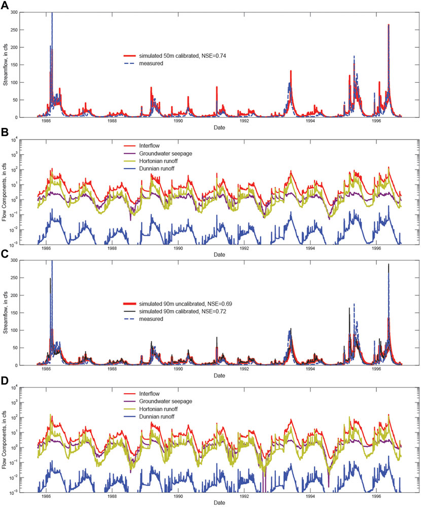
FIGURE 7. Sagehen Creek test model (Larsen et al., 2021) results showing comparisons between simulated and measured streamflow (10,343,500 SAGEHEN C NR TRUCKEE CA; U.S. Geological Survey, 2021) and contributions to streamflow for (A,B) 50 m × 50 m, and (C,D) 90 m × 90 m model cell sizes, respectively. All flows correspond to the location of the streamgage at the outlet of the watershed shown in Figure 6. Part (C) shows simulated versus measured flows for parameters unchanged from the 50 m calibration used in the 90 m calibration and the calibrated 90 m simulation.

Because the 50 m model was calibrated to the measured streamflow, and these parameter values were transferred directly to the 90 m model, the effect of grid size on simulated streamflow can be isolated and evaluated. The results confirm previous research that indicates larger grid cells tend to slightly increase dispersion and attenuate peak flow events (Sulis et al., 2010), and because the model was calibrated using the 50 m model, this attenuation results in a slight underprediction of peak flow in the 90 m model. The daily Nash-Sutcliffe Efficiency (NSE) values are equal to 0.74 and 0.69 for the 50 and 90 m models, respectively, when the 50 m calibrated parameters are transferred unchanged to the 90 m model. Calibrated results for the 90 m model show that a slightly better NSE is obtained with the finer discretization, where NSE is 0.72 and 0.74 for the calibrated 90 m and calibrated 50 m models (comparison between subparts 7a and 7c). Note that the slight reduction in the NSE value for the 90 m model is a result of changes in the magnitude of Hortonian runoff and groundwater discharge to the stream network shown in Figures 7B,D. This example illustrates the value of using automated model construction approaches like that provided by pyGSFLOW to quickly evaluate how different model resolutions impact hydrologic prediction, a process that is time consuming and prohibitive using conventional model construction approaches. The pyGSFLOW package provides an automated and efficient approach for evaluating the impacts of model conceptualization on predictions that allow the user to optimize model construction and quickly balance different factors, such as the tradeoff between fine spatial discretization and accuracy versus model computational costs. Increases in cell size from 50 to 90 m resulted in slightly lower Nash-Sutcliffe Efficiency, 0.74 to 0.72; however, this small sacrifice in accuracy is balanced by the significant reduction in computation time from 603 to 294 s.

Summary and Conclusion

GSFLOW models simulate complex interactions between surface-water and groundwater flow systems and require large data sets from many sources to fully parameterize. This paper presents methods that outline GSFLOW integrated hydrologic model development from raster digital elevation data to running model with pyGSFLOW. This approach builds on previous works (Bakker et al., 2016; Gardner et al., 2018; Larsen et al., 2021; Bakker et al., 2022) to create an open-source method for building PRMS, MODFLOW, and ultimately GSFLOW models. Flow direction, flow accumulation, watershed and subbasin delineation, and model building methods were developed specifically for use with tightly coupled GSFLOW models. Two example problems are presented to illustrate the robustness of the approach and illustrate the model construction process using pyGSFLOW.

The “Russian River Watershed Example” presents a regional system that is characterized by large areas of digitally flat digital elevation model (DEM), low-relief terrain with steep canyon walls that creates digital artifacts in the DEM data, and areas with high-relief topography. The D8 flow direction algorithm implemented in pyGSFLOW was used to define flow vectors within the watershed and ultimately be used to define subbasin boundaries and a model stream network. Results from this study showed that 1) pyGSFLOW’s modified Dijkstra algorithm is well suited for solving systems with large digitally flat expanses, like the Russian River; 2) the standard topological D8 flow direction method is ill suited for performing this task; and 3) the results are comparable but slightly different than both NHDPlus streamlines and ArcGIS’s flow accumulation methods. Differences between NHDPlus and pyGSFLOW’s results are explained by DEM scale mismatches between the model spatial discretization and NHDPlus streamlines.

The “Sagehen Creek Watershed Example” illustrates the step-by-step approach to developing input data required for a GSFLOW application. The python scripts are summarized here and provided in the pyGSFLOW repository to walk the user through the model development process using pyGSFLOW, including the processing of raster data to provide model parameters for both the PRMS and MODFLOW components of GSFLOW. This example compares two models created by varying spatial discretization with pyGSFLOW’s model building tools (Table 3). The first model has 50 m × 50 m grid cells, and the second model has 90 m × 90 m grid cells. The 90 m × 90 m model was quickly produced from a copy of the 50 m × 50 m model by changing only the spatial discretization of the model. Comparison of the two models shows that larger grid cells impact both the surface-water and groundwater components of simulated streamflow. Additional calibration beyond the parameterization of the 50 m model could be applied to the 90 m model to compensate for the deterioration in model fit when compared to the finer discretization model.

The pyGSFLOW package is currently being used to develop GSFLOW models of hydrologic watersheds in California to support groundwater sustainability and for tools that water managers can use to better manage surface water and groundwater as a single resource. Some example applications include, but are not limited to, evaluating different land-management or land-use scenarios, evaluating climate scenarios under historical or future conditions, parameter estimation, and sensitivity analysis. Because pyGSFLOW is a programmatic method for model creation, editing, and postprocessing, these applications can be accomplished by either creating a comprehensive script or with a series of scripts. Both options can be used for repeatable, transferable, and transparent model development.

The pyGSFLOW package is an open-source project that welcomes community input and involvement. The Russian River watershed and Sagehen Creek watershed example problems discussed in this paper can be found as python scripts in the pyGSFLOW repository (Larsen et al., 2021). Installation instructions, example problems, and links to documentation that demonstrate model building, editing existing models, and output data visualization can be accessed from the pyGSFLOW repository.

Data Availability Statement

The datasets presented in this study can be found in online repositories. The names of the repository/repositories and accession number(s) can be found below: https://code.usgs.gov/water/pyGSFLOW/-/tree/master/examples/frontiers and https://code.usgs.gov/water/pyGSFLOW/-/tree/master/examples.

Author Contributions

JL worked as lead software developer and lead author. AA has been a lead developer on the pyGSFLOW methods and authored sections of this article. DM developed approximately 50% of the new pyGSFLOW model building methods described and created the figures for this work. RN provided guidence on this work, calibrated the example problems, and authored parts of the article.

Funding

This work was funded by the USGS’s Water Availability and Use Program, the California State Water Resources Control Board, and Sonoma County Water Agency.

Author Disclaimer

Any use of trade, product, or firm names is for descriptive purposes only and does not imply endorsement by the U.S. Government.

Conflict of Interest

The authors declare that the research was conducted in the absence of any commercial or financial relationships that could be construed as a potential conflict of interest.

The handling editor declared a past co-authorship with one of the authors AA.

Publisher’s Note

All claims expressed in this article are solely those of the authors and do not necessarily represent those of their affiliated organizations, or those of the publisher, the editors and the reviewers. Any product that may be evaluated in this article, or claim that may be made by its manufacturer, is not guaranteed or endorsed by the publisher.

Acknowledgments

The authors welcome additions, suggestions, and assistance from the scientific community, and thank all past contributors for their work.

References

Bakker, M., Post, V., Hughes, J. D., Langevin, C. D., White, J. T., Leaf, A. T., et al. (2022). FloPy v3.3.6 — Release Candidate. U.S. Geological Survey Software Release. doi:10.5066/F7BK19FH

CrossRef Full Text | Google Scholar

Bakker, M., Post, V., Langevin, C. D., Hughes, J. D., White, J. T., Starn, J. J., et al. (2016). Scripting MODFLOW Model Development Using Python and FloPy. Groundwater 54, 733–739. doi:10.1111/gwat.12413

PubMed Abstract | CrossRef Full Text | Google Scholar

Beven, K. (2019). How to Make Advances in Hydrological Modelling. Hydrology Res. 50, 1481–1494. doi:10.2166/nh.2019.134

CrossRef Full Text | Google Scholar

Blöschl, G., Bierkens, M. F., Chambel, A., Cudennec, C., Destouni, G., Fiori, A., and Renner, M. (2019). Twenty-three Unsolved Problems in Hydrology (UPH)–a Community Perspective. Hydrological Sci. J. 64, 10. doi:10.1080/02626667.2019.1620507

CrossRef Full Text | Google Scholar

Buto, S. G., and Anderson, R. D. (2020). NHDPlus High Resolution (NHDPlus HR)---A Hydrography Framework for the Nation. Reston, VA: U.S. Geological Survey. Fact Sheet 2020-3033. doi:10.3133/fs20203033

CrossRef Full Text | Google Scholar

Clark, M. P., Kavetski, D., and Fenicia, F. (2011). Pursuing the Method of Multiple Working Hypotheses for Hydrological Modeling. Water Resour. Res. 47, 9. doi:10.1029/2010WR009827

CrossRef Full Text | Google Scholar

Condon, L. E., and Maxwell, R. M. (2015). Evaluating the Relationship between Topography and Groundwater Using Outputs from a Continental-Scale Integrated Hydrology Model. Water Resour. Res. 51, 6602–6621. doi:10.1002/2014WR016774

CrossRef Full Text | Google Scholar

Dijkstra, E. W. (1959). A Note on Two Problems in Connexion with Graphs. Numer. Math. 1, 269–271. doi:10.1007/BF01386390

CrossRef Full Text | Google Scholar

Garbrecht, J., and Martz, L. W. (1997). The Assignment of Drainage Direction over Flat Surfaces in Raster Digital Elevation Models. J. Hydrology 193, 204–213. doi:10.1016/S0022-1694(96)03138-1

CrossRef Full Text | Google Scholar

Gardner, M. A., Morton, C. G., Huntington, J. L., Niswonger, R. G., and Henson, W. R. (2018). Input Data Processing Tools for the Integrated Hydrologic Model GSFLOW. Environ. Model. Softw. 109, 41–53. doi:10.1016/j.envsoft.2018.07.020

CrossRef Full Text | Google Scholar

Goodchild, M. F. (2011). Scale in GIS: An Overview. Geomorphology 130, 5–9. doi:10.1016/j.geomorph.2010.10.004

CrossRef Full Text | Google Scholar

Harbaugh, A. W., Banta, E. R., Hill, M. C., and McDonald, M. G. (2000). MODFLOW-2000, the U.S. Geological Survey Modular Ground-Water Model – User Guide to Modularization Concepts and the Ground-Water Flow Process. Reston, VA: U.S. Geological Survey. Open-File Report 00-92. doi:10.3133/ofr200092

CrossRef Full Text | Google Scholar

Harbaugh, A. W. (2005). “MODFLOW-2005 : the U.S. Geological Survey Modular Ground-Water Model-Tthe Ground-Water Flow Process,” in Techniques and Methods 6-A16 (Reston, VA: U.S. Geological Survey). doi:10.3133/tm6A16

CrossRef Full Text | Google Scholar

Hay, L. E., Leavesley, G. H., Clark, M. P., Markstrom, S. L., Viger, R. J., and Umemoto, M. (2006). Step Wise, Multiple Objective Calibration of a Hydrologic Model for a Snowmelt Dominated Basin. J. Am. Water Resour. Assoc. 42 (4), 877–890. doi:10.1111/j.1752-1688.2006.tb04501.x

CrossRef Full Text | Google Scholar

Henson, W. R., Medina, R. L., Mayers, C. J., Niswonger, R. G., and Regan, R. S. (2013). “CRT—Cascade Routing Tool to Define and Visualize Flow Paths for Grid-Based Watershed Models,” in Techniques and Methods 6-D2 (Reston, VA: U.S. Geological Survey), 28.

Google Scholar

Huntington, J. L., and Niswonger, R. G. (2012). Role of Surface-Water and Groundwater Interactions on Projected Summertime Streamflow in Snow Dominated Regions: An Integrated Modeling Approach. Water Resour. Res. 48, 11. doi:10.1029/2012WR012319

CrossRef Full Text | Google Scholar

Jenson, S. K., and Domingue, J. O. (1988). Extracting Topographic Structure from Digital Elevation Data for Geographic Information System Analysis. Photogrammetric Eng. remote Sens. 54 (11), 1593–1600.

Google Scholar

Kahn, A. B. (1962). Topological Sorting of Large Networks. Commun. ACM 5, 558–562. doi:10.1145/368996.369025

CrossRef Full Text | Google Scholar

Kampf, S. K., and Burges, S. J. (2007). A Framework for Classifying and Comparing Distributed Hillslope and Catchment Hydrologic Models. Water Resour. Res. 43, 5. doi:10.1029/2006WR005370

CrossRef Full Text | Google Scholar

Kitlasten, W., Morway, E. D., Niswonger, R. G., Gardner, M., White, J. T., Triana, E., et al. (2021). Integrated Hydrology and Operations Modeling to Evaluate Climate Change Impacts in an Agricultural Valley Irrigated with Snowmelt Runoff. Water Resour. Res. 57, 6. doi:10.1029/2020WR027924

CrossRef Full Text | Google Scholar

Konikow, L. F., and Kendy, E. (2005). Groundwater Depletion: A Global Problem. Hydrogeol. J. 13 (1), 317–320. doi:10.1007/s10040-004-0411-8

CrossRef Full Text | Google Scholar

LANDFIRE (2016). Data from: LANDFIRE Existing Vegetation Type Layer. Reston, VA: U.S.Department of Interior, Geological Survey, and U.S. Department of Agriculture. Available at: http://landfire.cr.usgs.gov/viewer/.

Google Scholar

Larsen, J. D., Alzraiee, A., and Niswonger, R. G. (2022). Integrated Hydrologic Model Development and Postprocessing for GSFLOW Using pyGSFLOW. J. Open Source Softw. 7, 3852. 72. doi:10.21105/joss.03852

CrossRef Full Text | Google Scholar

Larsen, J. D., Alzraiee, A., and Niswonger, R. (2021). pyGSFLOW v1.0.0. U.S. Geological Survey Software Release. doi:10.5066/P9NPZ5AD

CrossRef Full Text | Google Scholar

Leaf, A. T., Fienen, M. N., and Reeves, H. W. (2021). SFRmaker and Linesink-Maker: Rapid Construction of Streamflow Routing Networks from Hydrography Data. Groundwater 59, 761–771. doi:10.1111/gwat.13095

CrossRef Full Text | Google Scholar

Maidment, D. R., and Morehouse, S. (2002). Arc Hydro: GIS for Water Resources. Redlands, CA: ESRI, Inc.

Google Scholar

Mark, D. M. (1988). “Network Models in Geomorphology,” in Modelling in Geomorphological Systems. Editor M. G. Anderson (Chichester [West Sussex], NY: John Wiley), 73–97.

Google Scholar

Markstrom, S. L., Niswonger, R. G., Regan, R. S., Prudic, D. E., and Barlow, P. M. (2008). GSFLOW-coupled Ground-Water and Surface-Water FLOW Model Based on the Integration of the Precipitation-Runoff Modeling System (PRMS) and the Modular Ground-Water Flow Model (MODFLOW-2005). Reston, VA: U.S. Geological Survey, 240. Techniques and Methods 6-D1.

Google Scholar

Markstrom, S. L., Regan, R. S., Hay, L. E., Viger, R. J., Webb, R. M. T., Payn, R. A., et al. (2015). PRMS-IV, the Precipitation-Runoff Modeling System, Version 4. Reston, VA: U.S. Geological Survey, 158. Techniques and Methods, book 6, chap. B7.

Google Scholar

Martz, L. W., and Garbrecht, J. (1999). An Outlet Breaching Algorithm for the Treatment of Closed Depressions in a Raster DEM. Comput. Geosciences 25, 835–844. doi:10.1016/s0098-3004(99)00018-7

CrossRef Full Text | Google Scholar

Metz, M., Mitasova, H., and Harmon, R. S. (2011). Efficient Extraction of Drainage Networks from Massive, Radar-Based Elevation Models with Least Cost Path Search. Hydrol. Earth Syst. Sci. 15, 667–678. doi:10.5194/hess-15-667-2011

CrossRef Full Text | Google Scholar

National Land Cover Database (NLCD). (2020). Data from: 2016 Shrubland Fractional Components for the Western U.S. doi:10.5066/P9MJVQSQ

CrossRef Full Text | Google Scholar

Ng, G.-H. C., Wickert, A. D., Somers, L. D., Saberi, L., Cronkite-Ratcliff, C., Niswonger, R. G., et al. (2018). GSFLOW-GRASS v1.0.0: GIS-Enabled Hydrologic Modeling of Coupled Groundwater-Surface-Water Systems. Geosci. Model Dev. 11, 4755–4777. doi:10.5194/gmd-11-4755-2018

CrossRef Full Text | Google Scholar

Niswonger, R. G., Panday, S., and Ibaraki, M. (2011). MODFLOW-NWT, A Newton Formulation for MODFLOW-2005. Reston, VA: Geological Survey, 44. Techniques and Methods 6-A37. doi:10.3133/tm6A37

CrossRef Full Text | Google Scholar

Niswonger, R. G., and Prudic, D. E. (2005). Documentation of the Streamflow-Routing (SFR2) Package to Include Unsaturated Flow beneath Streams - A Modification to SFR1. Reston, VA: Geological Survey, 47. Techniques and Methods 6-A13. doi:10.3133/tm6A13

CrossRef Full Text | Google Scholar

Niswonger, R. G., Prudic, D. E., and Regan, R. S. (2006). Documentation of the Unsaturated-Zone Flow (UZF1) Package for Modeling Unsaturated Flow between the Land Surface and the Water Table with MODFLOW-2005. Reston, VA: U.S. Geological Survey, 62. Techniques and Methods 6-A19. doi:10.3133/tm6A19

CrossRef Full Text | Google Scholar

O’Callaghan, J. F., and Mark, D. M. (1984). The Extraction of Drainage Networks from Digital Elevation Data. Comput. Vis. Graph. Image Process. 28, 323–344. doi:10.1016/S0734-189X(84)80011-0

CrossRef Full Text | Google Scholar

PRISM Climate Group (2014). Data from: Prism Climate Group. Corvallis, OR: Oregon State University. Available at: https://prism.oregonstate.edu.

Google Scholar

Qin, C., Zhu, A. X., Pei, T., Li, B., Zhou, C., and Yang, L. (2007). An Adaptive Approach to Selecting a Flow-Partition Exponent for a Multiple-Flow-Direction Algorithm. Int. J. Geogr. Inf. Sci. 21, 443–458. doi:10.1080/13658810601073240

CrossRef Full Text | Google Scholar

Regan, R. S., Juracek, K. E., Hay, L. E., Markstrom, S. L., Viger, R. J., Driscoll, J. M., LaFontaine, J. H., and Norton, P. A. (2019). The U. S. Geological Survey National Hydrologic Model Infrastructure: Rationale, Description, and Application of a Watershed-Scale Model for the Conterminous United States. Environ. Model. Softw. 111, 192–203. doi:10.1016/j.envsoft.2018.09.023

CrossRef Full Text | Google Scholar

Schoups, G., Hopmans, J. W., Young, C. A., Vrugt, J. A., Wallender, W. W., Tanji, K. K., et al. (2005). Sustainability of Irrigated Agriculture in the San Joaquin Valley, California. Proc. Natl. Acad. Sci. U.S.A. 102, 15352–15356. doi:10.1073/pnas.0507723102

PubMed Abstract | CrossRef Full Text | Google Scholar

Schoups, G., Vrugt, J. A., Fenicia, F., and Van De Giesen, N. C. (2010). Corruption of Accuracy and Efficiency of Markov Chain Monte Carlo Simulation by Inaccurate Numerical Implementation of Conceptual Hydrologic Models. Water Resour. Res. 46, 10. doi:10.1029/2009WR008648

CrossRef Full Text | Google Scholar

Shin, S., Pokhrel, Y., and Miguez‐Macho, G. (2019). High‐Resolution Modeling of Reservoir Release and Storage Dynamics at the Continental Scale. Water Resour. Res. 55, 787–810. doi:10.1029/2018WR023025

CrossRef Full Text | Google Scholar

Sulis, M., Paniconi, C., and Camporese, M. (2010). Impact of grid resolution on the integrated and distributed response of a coupled surface-subsurface hydrological model for the des Anglais catchment, Quebec. Hydrol. Process. 25, 1853–1865. doi:10.1002/hyp.7941

CrossRef Full Text | Google Scholar

Tarboton, D. G. (1997). A New Method for the Determination of Flow Directions and Upslope Areas in Grid Digital Elevation Models. Water Resour. Res. 33, 309–319. doi:10.1029/96WR03137

CrossRef Full Text | Google Scholar

University of California Berkeley (2008). Data from: Sagehen Creek Field Station, UC Berkeley. Berkeley, CA: Historical Weather Data. Available at: https://wrcc.dri.edu/cgi-bin/rawMAIN.pl?nvsagh.

Google Scholar

U.S. Geological Survey (2020). Data from: 3D Elevation Program 1-Meter Resolution Digital Elevation Model. Available at: https://elevation.nationalmap.gov/arcgis/rest/services/3DEPElevation/ImageServer.

Google Scholar

U.S. Geological Survey (2021). Data from: National Water Information System Data Available on the World Wide Web (Water Data for the Nation). doi:10.5066/F7P55KJN

CrossRef Full Text | Google Scholar

U.S. Geological Survey (2022). Data from: USGS 3D Elevation Program Digital Elevation Model. Available at: https://elevation.nationalmap.gov/arcgis/rest/services/3DEPElevation/ImageServer.

Google Scholar

Volk, J. M., and Turner, M. A. (2019). PRMS-Python: A Python Framework for Programmatic PRMS Modeling and Access to Its Data Structures. Environ. Model. Softw. 114, 152–165. doi:10.1016/j.envsoft.2019.01.006

CrossRef Full Text | Google Scholar

Wada, Y., Van Beek, L. P. H., Van Kempen, C. M., Reckman, J. W. T. M., Vasak, S., and Bierkens, M. F. P. (2010). Global Depletion of Groundwater Resources. Geophys. Res. Lett. 37, L20402. doi:10.1029/2010GL044571

CrossRef Full Text | Google Scholar

Wang, L., and Liu, H. (2006). An Efficient Method for Identifying and Filling Surface Depressions in Digital Elevation Models for Hydrologic Analysis and Modelling. Int. J. Geogr. Inf. Sci. 20, 193–213. doi:10.1080/13658810500433453

CrossRef Full Text | Google Scholar

Wang, Y., Liu, Y., Xie, H., and Xiang, Z. (2011). “A Quick Algorithm of Counting Flow Accumulation Matrix for Deriving Drainage Networks from a DEM,” in Proceedings on the Third International Conference on Digital Image Processing. doi:10.1117/12.896274

CrossRef Full Text | Google Scholar

Werner, A. D., Gallagher, M. R., and Weeks, S. W. (2006). Regional-scale, Fully Coupled Modelling of Stream-Aquifer Interaction in a Tropical Catchment. J. Hydrology 328, 497–510. doi:10.1016/j.jhydrol.2005.12.034

CrossRef Full Text | Google Scholar

Wood, E. F., Lettenmaier, D., Liang, X., Nijssen, B., and Wetzel, S. W. (1997). Hydrological Modeling of Continental-Scale Basins. Annu. Rev. Earth Planet. Sci. 25, 279–300. doi:10.1146/annurev.earth.25.1.279

CrossRef Full Text | Google Scholar

Zhang, H., Yao, Z., Yang, Q., Li, S., Baartman, J. E. M., Gai, L., et al. (2017). An Integrated Algorithm to Evaluate Flow Direction and Flow Accumulation in Flat Regions of Hydrologically Corrected DEMs. Catena 151. doi:10.1016/j.catena.2016.12.009

CrossRef Full Text | Google Scholar