Forecasting of monthly precipitation based on ensemble empirical mode decomposition and Bayesian model averaging

1 Introduction

Precipitation is an essential input for hydrologic simulation and prediction, which is widely used in activities such as agriculture, water resource management and flood forecasting (Kang et al., 2020). The climate continues to warm with rapid socio-economic development, population growth, and a dramatic increase in greenhouse gases. Extreme precipitation and extreme drought events are occurring more and more frequently, seriously threatening people’s lives and property. Accurate precipitation prediction can provide preparation time and decision basis for authorities to cope with potential disasters. Due to the complexity and variability of meteorological conditions, it is very difficult to predict precipitation accurately. Until now, there have been two main types of prediction models for precipitation: process-based models and data-driven models. Process-based models require large amounts of data on physical parameters, while data-driven models require only historical observations and are easy to implement. Data-driven models have been widely adopted in hydrological forecasting with excellent results. Lai and Dzombak (2020) used an Autoregressive Integrated Moving Average model (ARIMA) model to predict temperature and precipitation. Their results showed that ARIMA models are generally more accurate than other forecasting models, especially with interval predictions. However, the ARIMA model only works well when the time series is stationary. Recently, various machine learning models, such as Support Vector Regression (SVR) (Wang et al., 2019), Artificial Neural Networks (ANN) (Cheng et al., 2015; Jabbari and Bae, 2018), and Adaptive Neuro Fuzzy Inference System (ANFIS) (Jimeno-Saez et al., 2017; Belvederesi et al., 2020), have been widely used for time series forecasting due to their powerful learning capabilities. Although these models can handle non-linear data, they ignore the sequential relationships between the data and their predictive performance needs to be improved.

The recurrent neural network (RNN) architecture contains feedback connections which allow the network to remember previous information. However, recurrent networks have difficulty learning long-term dependencies in sequences. Gradient disappearance and explosion problems occur when back-propagation errors flow through multiple time steps (Bengio et al., 1994). The Long Short-Term Memory (LSTM) neural network introduces a memory block to control the transmission and updating of information, effectively alleviating the problem of gradient disappearance (Hochreiter and Schmidhuber, 1997). Due to the power of LSTM to handle sequential problems, it has been widely used in time series prediction, speech recognition, sentiment analysis and natural language processing (Sundermeyer et al., 2015; Fischer and Krauss, 2018; Al-Smadi et al., 2019; Lippi et al., 2019). In the past few years, several studies have used LSTM for hydrological and meteorological prediction with good results. Kratzert et al. (2018) adopted LSTM to simulate rainfall-runoff and showed the potential of LSTM for hydrological modelling applications. Xu W. et al. (2020) used LSTM to predict river flow and achieved great results.

Data denoising can enhance the performance of data-driven models, and Ensemble Empirical Mode Decomposition (EEMD) is one of the most commonly used data denoising methods. The EEMD was proposed by Wu and Huang (2009), and effectively suppressed the mode mixing problem of the Empirical Mode Decomposition (EMD) method. Due to its simplicity and effectiveness, EEMD has been successfully applied for time series prediction. Kang et al. (2017) used the EEMD-LSSVM model to predict short-term wind speed and performed well in terms of the evaluation metrics selected. Tayyab et al. (2018) utilized the EEMD-RBF model to forecast streamflow in the Upper Indus basin, Pakistan. Their results indicated that the EEMD-RBF has better predictive capability. Wang et al. (2020) applied the EEMD-SVR and EEMD-ANN models for monthly flow series regression, and the regression results were more precise than regressing directly with the original series. However, the reconstruction error (RE) of the EEMD method, which represents the difference between the original sequence and the corresponding IMFs, affects the final prediction accuracy. The RE is often complex and unpredictable, but if we discard it, the final prediction will deviate somewhat from the original precipitation data.

In precipitation prediction studies, focusing only on model accuracy tends to ignore the risks associated with the uncertainty of the model itself. Draper (1995) proposed the Bayesian model averaging (BMA) method to solve the model uncertainty problem. BMA assigns appropriate weights to each base model, resulting in more robust prediction results. In addition, BMA can also obtain interval forecasts with certain probabilities, thus providing more useful information for decision makers. BMA has been widely used in research of hydrological ensemble forecasting (Jiang et al., 2018; Meira Neto et al., 2018; Xu L. et al., 2020).

In this study, a hybrid EEMD-BMA model, is proposed for monthly precipitation prediction. The monthly precipitation data series of Kunming Station in southwest China, from January 1951 to December 2020, is used as an example for the study. Section 2 contains the methods used in this study. Section 3 provides the results and analysis of precipitation projections. Section 4 summarizes the full paper.

2 Materials and methods

2.1 Study area and data

Kunming is the capital of Yunnan province and lies at the longitude of 102°10′-103°40′E and the latitude of 24°23′-26°22′N. The position of Kunming station is shown in Figure 1. Kunming is in a subtropical highland monsoon climate zone. The annual average temperature is approximately 15°C and the annual average precipitation is about 1000 mm. 90% of Kunming’s precipitation is concentrated between May and October and there are many heavy rainstorms, making it vulnerable to flooding.

FIGURE 1

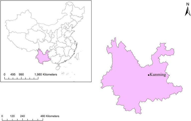
FIGURE 1. Location of the Kunming station.

In this study, monthly precipitation data from Kunming station was from the China Meteorological Data Service Centre (http://data.cma.cn) from January 1951 to December 2020. All monthly precipitation data is quality controlled and checked. The monthly precipitation data, as shown in Figure 2, fluctuates greatly. We used 70% of the entire dataset as the training set and 30% as the test set. The training set, ranging from January 1951 to December 1999 is used to build the model. The test set covers January 2000 to December 2020 and is used to evaluate the model prediction performance.

FIGURE 2

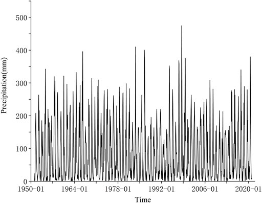
FIGURE 2. Monthly precipitation data of Kunming station from January 1951 to December 2020.

2.2 Ensemble empirical mode decomposition (EEMD)

The Empirical Mode Decomposition (EMD) method is an effective method to deal with non-stationary and non-linear signals (Huang et al., 1998). It decomposes the original signal into multiple intrinsic mode functions (IMFs) and a residue. Each IMF must satisfy the two rules: 1) The number of extrema in the entire signal data sequence must be equal to the number of zero crossing or differ at most by one; 2) The average value of the envelope defined by local maxima and minima must be zero at any point. The core of the EMD method is the screening process that generates IMFs, and the specific steps are as follows:

1) Determine all local extrema of the original signal data series $x\left(t\right)$.

2) Using the cubic spline interpolation function, generate the upper envelope $e_{up}\left(t\right)$ and lower envelope $e_{low}\left(t\right)$ of the original signal data series.

3) Calculate the mean value $m\left(t\right)$ of the envelopes. The average value $m\left(t\right)$ can be calculated as:

$m\left(t\right)=\frac{e_{up}\left(t\right)+e_{low}\left(t\right)}{2},(1)$

4) Obtain the difference $h\left(t\right)$ between the original signal sequence $x\left(t\right)$ and the mean value $m\left(t\right).h\left(t\right)$ can be calculated by the following formula:

$h\left(t\right)=x\left(t\right)-m\left(t\right),(2)$

5) Check $h\left(t\right)$: If $h\left(t\right)$ satisfies the two conditions of IMFs, indicating that $h\left(t\right)$ is an IMF, then repeat the above steps with $r\left(t\right)=x\left(t\right)-h\left(t\right)$ instead of $x\left(t\right)$; Otherwise, continue the above steps with $h\left(t\right)$ instead of $x\left(t\right)$.

6) The screening process is repeated until the stopping criterion is met. The stopping criterion can be achieved by limiting the size of the standard deviation (SD), which is calculated from two consecutive screening results:

$SD={\displaystyle \sum _{t=0}^T\left[\frac{{\left|h_{k-1}\left(t\right)-h_k\left(t\right)\right|}^2}{h_{k-1}^2\left(t\right)}\right]},(3)$

where k is the number of times the screening process takes place. When the SD is less than a predefined value, typically 0.2 to 0.3, the screening process stops. Finally, by summing all of the IMFs $c_i\left(t\right)$ and the residual item $r\left(t\right)$, we obtain

$x\left(t\right)={\displaystyle \sum _{i=0}^n{c}_i\left(t\right)+r\left(t\right)},(4)$

There are still some unavoidable drawbacks of EMD. One of the main problems is the mode mixing, which means that a single IMF is mixed with different frequency components, or different IMFs contain the same frequency component. The mode mixing problem seriously interferes with decomposition effect. The EEMD facilitates the separation of different scales of the input data by adding Gaussian white noise (Yuan et al., 2021). White noise helps to perturb original signal and enable the EMD algorithm to visit all possible solutions in the finite neighborhood of the true final answer (Wu and Huang, 2009). Due to the zero-mean characteristic of Gaussian white noise, after multiple averaging, the noises cancel each other out and give a better combined average result (Li et al., 2021). The main procedures of EEMD are as follow.

1) The original signal data sequence x(t) is supplemented with Gaussian white noise w_i(t). The new sequence can be calculated as:

$x_i\left(t\right)=x\left(t\right)+w_i\left(t\right),(5)$

2) Using the EMD sifting process, decompose the new data sequence into IMFs;

3) Repeat the preceding steps with different white noises;

4) Calculate the average values of the corresponding IMFs as the final results:

$c_j=\frac{1}{N}{\displaystyle \sum _{i=1}^N{c}_{j,i}},(6)$

where N is the ensemble times of adding noise, c_j reparents the jth IMF component; c_j,I is the ith IMF when adding the ith noise.

The impact of the added noise should abide by the statistical rules:

${\mathit{\epsilon }}_n=\frac{\mathit{\epsilon }}{\sqrt{N}},(7)$

Where N is the number of ensemble members, ε denotes the amplitude of the added noise, and ε_n represents the final standard deviation of RE.

2.3 Single models for precipitation prediction

We used a one-step ahead approach to predict precipitation. This means that previous $l$ data sample points P_t-1, P_t-2, … , P_t-l are used to predict the present data point P_t, where $l$ is the time step. ARIMA, SVR and LSTM are used for precipitation prediction. Since each IMF component corresponds to a different time step, resulting in different lengths of predictions, we retain the shortest length after aligning from back to front. Finally, the predictions of all components are summed to obtain the final precipitation forecast. As precipitation is non-negative, all negative values appearing in the precipitation forecasts are replaced by zero.

2.3.1 Autoregressive integrated moving average (ARIMA) model

The ARIMA model was introduced by Box and Jenkins. It has become a prominent method in time series analysis. ARIMA essentially relies on past values of the series and previous error terms for prediction (Adebiyi et al., 2014). It can be calculated as:

$Y_t={\varphi }_0+{\varphi }_1{Y}_{t-1}+{\varphi }_2{Y}_{t-2}+\cdots +{\varphi }_p{Y}_{t-p}+{\epsilon }_t+{\theta }_1{\epsilon }_{t-1}+{\theta }_2{\epsilon }_{t-2}+\cdots +{\theta }_q{\epsilon }_{t-q},(8)$

Where Y_t is the actual value and ε_t is the random error at time t, p and q are the order of the autoregressive and moving average, respectively.

2.3.2 Support vector regression (SVR)

The basic idea of support vector machine (SVM) is to map the sample space to a high-dimensional space by a kernel function, so that samples that cannot be accurately classified in the original sample space become linearly separable in the high-dimensional feature space. Support vector regression (SVR) is a regression method developed from SVM. The regression function is as follows:

$f\left(x\right)={\displaystyle \sum _{i=1}^n\left({\alpha }_i^{\ast }-{\alpha }_i\right)K\left(x_i,x_j\right)+b},(9)$

Where α_i^* and α_i are the Lagrange multipliers; K (x_i, x_j) is the kernel function; b is bias.

2.3.3 Long short-term memory (LSTM) neural network

Traditional RNNs encounter the problem of gradient disappearance when dealing with long-term dependency problem. To overcome this problem, Hochreiter and Schmidhuber (1997) proposed the long short-term memory (LSTM) neural network. Due to the strength of the LSTM in discovering long-term dependencies, it is widely used in the processing of sequence information.

The main advantage of LSTM over the traditional RNN is that LSTM adds a memory cell to store information and three gates to control the delivery and updating of information. The exact calculation steps of the LSTM are as follows:

$f_t=\mathit{\sigma }\left(W_f\cdot \left[h_{t-1},x_t\right]+b_f\right),(10)$

$i_t=\mathit{\sigma }\left(W_i\mathrm{\cdot }\left[h_{t-1},x_t\right]+b_i\right),(11)$

$g_t=\tanh \left(W_c\mathrm{\cdot }\left[h_{t-1},x_t\right]+b_c\right),(12)$

$C_t=f_t\mathrm{\ast }{C}_{t-1}+i_t\mathrm{\ast }{g}_t,(13)$

$o_t=\mathit{\sigma }\left(W_o\mathrm{\cdot }\left[h_{t-1},x_t\right]+b_o\right),(14)$

$h_t=o_t\mathrm{\ast }\tanh \left(c_t\right),(15)$

Where f_t, i_t, o_t are the outputs of forget gate, input gate and output gate; x_t is the input; h_t is the outputs of the hidden layer; C_t is the cell state; g_t is the candidate state of the cell; W_f, W_i, W_o, W_c are the weights; b_f, b_i, b_o and b_c are the bias terms.

2.4 Bayesian model averaging (BMA)

The BMA method ensembles individual models using posterior probabilities as weights, effectively dealing with the model uncertainty problem (Draper, 1995). The basic principle of BMA is as follows.

Suppose y is the forecast value of BMA, the data set D consists of the forecast results and the actual precipitation, and M = [M₁, M₂, …, M_k] is the model space consisting of all possible models. Then the posterior distribution of y can be expressed as:

$p\left(y|D\right)={\displaystyle \sum _{k=1}^{K}p\left(M_k|D\right)p_k\left(y|M_k,D\right)},(16)$

Where M_k represents the kth model in the model space; K denotes the number of models contained in the model space. $p\left(M_k|D\right)$ is the posterior probability of M_k,.

The $p\left(M_k|D\right)$ can be calculated by the following equation:

$P\left(M_k|D\right)=\frac{P\left(D|M_k\right)P\left(M_k\right)}{{\displaystyle \sum _{k=1}^{K}P\left(D|M_k\right)P\left(M_k\right)}},(17)$

where $P\left(D|M_k\right)$ denotes the integral of the likelihood function corresponding to model M_k; p (M_k) is the prior probabilities of model M_j.

The posterior mean and variance can be expressed as:

$E\left[y|D\right]={\displaystyle \sum _{k=1}^{K}E\left[y|M_k,D\right]}p\left(M_k|D\right)={\displaystyle \sum _{k=1}^K{w}_k{M}_k},(18)$

$Var\left[y|D\right]={{\displaystyle \sum _{k=1}^K\left(M_k-{\displaystyle \sum _{k=1}^K{w}_k{M}_k}\right)}}^2+{\displaystyle \sum _{k=1}^K{w}_k{\sigma }_k^2},(19)$

Where σ_k² is the variance of M_k.

The posterior probability distribution of BMA often involves the computation of complex high-dimensional integrals. Markov Chain Monte Carlo (MCMC) is a good way to solve this problem. The basic idea of MCMC is to build a Markov chain with a smooth distribution π(x) that is a good approximation of the posterior distribution. After a period of pre-iterations, a series of simulated values of the Markov chain is generated, which can be considered as independent samples from the posterior distribution. Various statistical inferences can then be made based on these samples. Due to its high efficiency and robustness, MCMC has been widely used in many fields (Pérez et al.,2006; Ching and Chen, 2007; Zhao and Wang, 2020). In this study, the BMA method was implemented using the BMS package in R (Zeugner, 2011). A birth-death MCMC algorithm (Stephens, 2000) was used to wander through model space by adding or dropping regressors from the current model. The number of iterations was set to 200,000 to ensure that the Markov chain reached a steady state.

2.5 The EEMD-BMA model

Precipitation data is highly nonlinear and nonstationary, which makes it difficult to accurately predict with a single model. We used a hybrid EEMD-BMA model to predict monthly precipitation data. The process of EEMD-BMA is shown in Figure 3. The specific procedures are as follows:

1) The decomposition of monthly precipitation data series: The EEMD method was used to decompose the original monthly precipitation sequences into multiple IMFs and a residue.

2) Determination of time step: The input time step was obtained using the PACF algorithm.

3) Predicting of IMFs and residue: Build proper ARIMA, SVR and LSTM models for components.

4) Predicting of reconstruction error: According to Eq. 7, the standard deviation of the reconstruction error can be kept small by appropriately increasing the number of times white noise is added. In this way, we can obtain relatively accurate prediction results by using the average value of the training set of reconstruction error as the prediction value of its test set.

5) Reconstruction of predicted results: The respective predictions were summed to obtain the predictions of monthly precipitation by the EEMD-ARIMA, EEMD-SVR and EEMD-LSTM models.

6) Weighted average of predicted results: Averaging the results of EEMD-ARIMA, EEMD-SVR and EEMD-LSTM by BMA.

7) Evaluate model performance: The model’s predicted results are compared with real precipitation. Evaluate the performance of the EEMD-BMA model based on several statistical metrics.

FIGURE 3

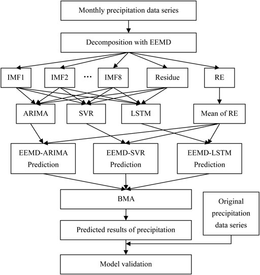
FIGURE 3. The workflow Chart of EEMD-BMA.

2.5.1 Statistical assessment indicators for predicting performance

Four evaluation metrics were used in this study to assess the predictive accuracy of the models. They include mean square error (MSE), root mean square error (RMSE), mean absolute error (MAE), and coefficient of determination (R²). MSE, RMSE, MAE indicate the magnitude of errors between original precipitation and predicted results. The smaller their values are, the higher the accuracy of the model. R² is a measure for the degree of model fit. The closer R² is to 1, the higher the degree of fit between the predicted and actual precipitation. The corresponding formulas are as follows:

$\text{MSE}=\frac{1}{n}{{\displaystyle \sum _{i=1}^n\left(P_i-P_i^{\mathrm{\ast }}\right)}}^2,(20)$

$\text{RMSE}=\sqrt{\frac{1}{n}{{\displaystyle \sum _{i=1}^n\left(P_i-P_i^{\mathrm{\ast }}\right)}}^2},(21)$

$\text{MAE}=\frac{1}{n}{\displaystyle \sum _{i=1}^n\left|P_i-P_i^{\mathrm{\ast }}\right|},(22)$

${\text{R}}^2=1-\frac{{{\displaystyle \sum _{i=1}^n\left(P_i-P_i^{\mathrm{\ast }}\right)}}^2}{{{\displaystyle \sum _{i=1}^n\left(P_i-\overline{P}\right)}}^2},(23)$

Where $P_{\text{i}}$ and $P_i^{\mathrm{\ast }}$ are the observed and predicted values of precipitation at time $i$, respectively; n is the number of data sample points; $\overline{P}$ represents the average of the observed values.

The coverage probability (CP) and mean width (MW) are used in this paper to assess the suitability of BMA prediction intervals. The formulas are as follows:

$CP=\frac{C}{N}\times 100\%,(24)$

$MW=\frac{1}{N}{\displaystyle \sum _{i=1}^N\left(u{p}_i-dow{n}_i\right)},(25)$

Where C is the number of sample points covered by the BMA prediction interval; up_i and down_i are the upper and lower bounds of the BMA prediction interval, respectively.

3 Results and discussion

3.1 Decomposition results with EEMD

Choosing the appropriate ensemble times and amplitude of the added noise is crucial for EEMD decomposition. We tried different combinations of noise amplitudes and ensemble times, and found that the RE always existed. Reducing the noise amplitude makes the RE smaller, but too small amplitudes cannot separate out the different time scales in the original precipitation series and may lead to serious mode mixing problems. Thus, we choose a larger amplitude and increase the ensemble times. This ensures that the decomposition is effective while keeping the fluctuations in RE within a small range.

The original precipitation data is decomposed into eight IMFs and one residue by EEMD (Figure 4). As can be seen in Figure 4, the eight IMF components are arranged in decreasing order from high to low frequencies. The residue reflects the change trend of precipitation at Kunming station. Compared with the original precipitation series, the fluctuations of each component are more regular. After the EEMD decomposition, the model can better identify the variation characteristics of each component, which helps to improve the prediction performance. Statistics of the monthly precipitation series and decomposition results at Kunming station are given in Table 1. The standard deviations of the components are smaller than the original precipitation data, indicating that the components are more stable.

FIGURE 4

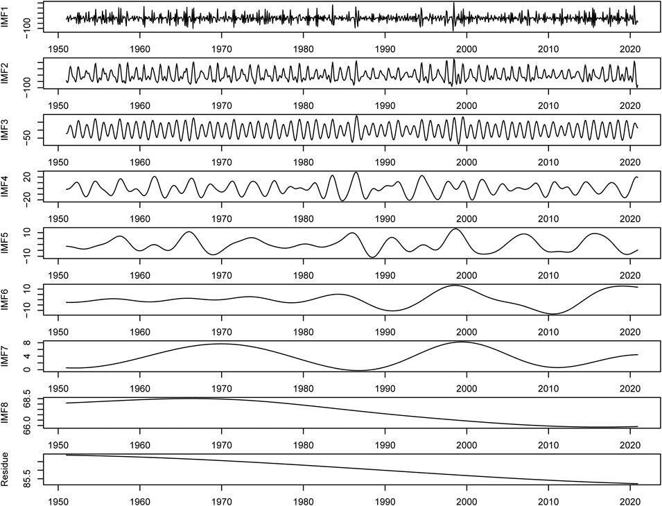
FIGURE 4. The decomposition results of the precipitation series at Kunming station by EEMD.

TABLE 1

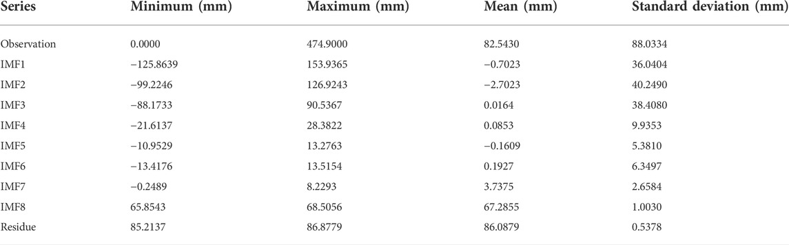
TABLE 1. Descriptive statistics of EEMD decomposition results.

The RE of EEMD fluctuates dramatically around its mean value (Figure 5). The standard deviation of the RE is relatively small. Therefore, we can get relatively good results by using the mean of the RE as its predicted value.

FIGURE 5

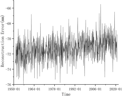
FIGURE 5. The reconstruction error (RE) of the precipitation series at Kunming station by EEMD.

3.2 Input time step of components

In this study, the partial autocorrelation function (PACF) is applied to determine the input time step. The PACF is effective in identifying correlation between the present value and several previous values of the series (Zhang et al., 2018). By calculating the partial autocorrelation coefficients of the decomposition results, their lag orders can be obtained. The PACF plots for the decomposition results of Kunming station are shown in Figure 6. The number of lags beyond the 95% confidence level (dotted line) is the input time step. As can be seen from Figure 6, the input time steps for the IMFs of Kunming station are 12,8,7,4,5,8,5,1 and 1.

FIGURE 6

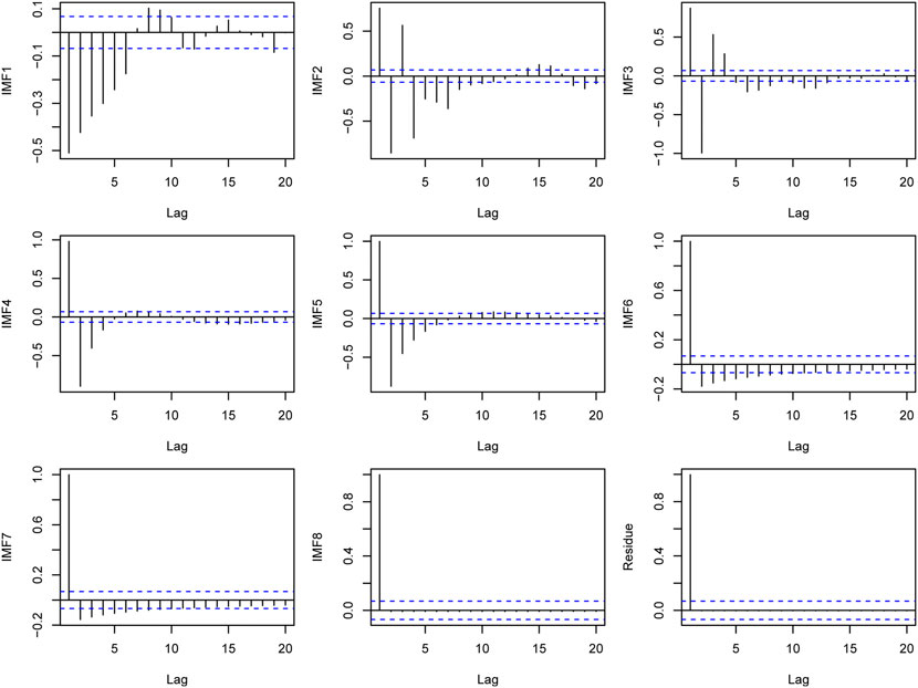
FIGURE 6. The PACF plots for the decomposition results of Kunming station.

3.3 Prediction results of individual model

We have obtained point prediction results for precipitation using ARIMA, SVR, LSTM, EEMD-ARIMA, EEMD-SVR and EEMD-LSTM. The predictions are shown in Figure 7. It is clear that all hybrid models perform better than the single models. The reason is that there are many abrupt changes in the precipitation series that are not well identified by the single models. By decomposing the precipitation data into a series of relatively stable components with the EEMD method, these models are able to identify local variations in the components, thus improving prediction accuracy. In addition, the EEMD-LSTM predictions are the closest to the original data of all the models, particularly at the extremes of the precipitation series. This indicates that the EEMD-LSTM model performed best in the one-step prediction of precipitation.

FIGURE 7

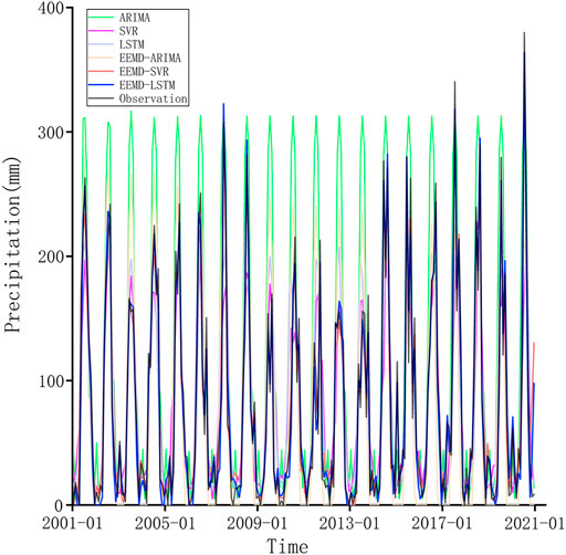
FIGURE 7. Comparison of the predicted results among ARIMA, SVR, LSTM, EEMD-ARIMA, EEMD-SVR, and EEMD-LSTM.

The scatterplots of the ARIMA, SVR, LSTM, EEMD-ARIMA, EEMD-SVR, and EEMD-LSTM model predictions versus the true precipitation at the Kunming station are shown in Figure 8. As can be seen from the plots, the single model predictions are far from the 45^o line, which shows that the three single models have poor prediction accuracy, with the ARIMA model showing the worst results. However, the hybrid models perform better than the single models, indicating that the EEMD can improve prediction accuracy. The predictions of the EEMD-LSTM model are closest to the 45^o line, indicating that the predicted values of the EEMD-LSTM have the highest correlation with actual precipitation.

FIGURE 8

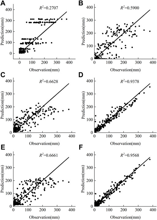
FIGURE 8. Scatter plots of prediction and observation (A) ARIMA (B) EEMD-ARIMA (C) SVR (D) EEMD-SVR (E)LSTM (F) EEMD-LSTM.

3.4 Predictied results of the EEMD-BMA model

To reduce uncertainty in precipitation predictions, we applied BMA to average the single models and the hybrid models respectively. The results of BMA are listed in Table 2. In Table 2, PIP is the post inclusion probabilities; Post Mean denotes the posterior expected value of coefficients, which is the weight assigned by BMA; Post SD is the posterior standard deviation of coefficients. The SVR model has the largest weight, which is 0.5235. the LSTM model has the smallest weight, which is 0.0322.

TABLE 2

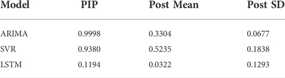
TABLE 2. Results of BMA.

Figure 9 shows the results of BMA with three single models. It can be noticed that the ensemble mean of BMA is relatively consistent with the trend of observed precipitation. However, for the peaks of the precipitation series, the results of the BMA are subject to large errors. In addition, the width of the 90% confidence interval for the ensemble mean of the BMA is large, indicating that there is still a large uncertainty in the predictions after BMA. This is because single models are unable to accurately identify the pattern of variability in monthly precipitation series and their predictions are not robust, which affects the effectiveness of the BMA.

FIGURE 9

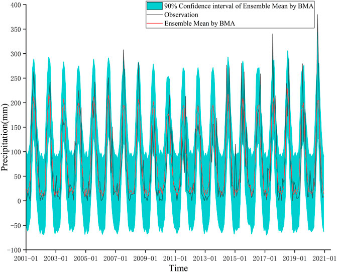
FIGURE 9. Results of BMA with three single models.

The results of EEMD-BMA are shown in Table 3. The EEMD-LSTM model has the largest weight of 0.9353, indicating that the predicted results of EEMD-LSTM contribute more to the BMA. The weight of EEMD-ARIMA model is close to zero, which means that the predicted results of EEMD-ARIMA contribute little to the BMA.

TABLE 3

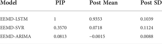
TABLE 3. Results of EEMD-BMA

The results of EEMD-BMA are shown in Figure 10. The ensemble mean is very close to the observation, indicating that the BMA can concentrate the strengths of the different models to obtain more accurate predictions. In addition, the 90% confidence interval of the ensemble mean by EEMD-BMA is narrower than that of BMA with single models, indicating that the hybrid models have less uncertainty. Moreover, extreme precipitation events almost fall within the 90% confidence interval of the EEMD-BMA.

FIGURE 10

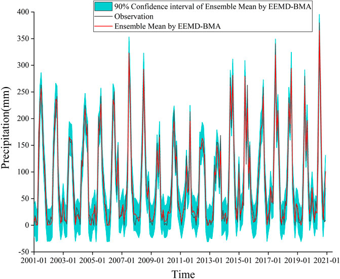
FIGURE 10. Results of the EEMD-BMA

3.5 Prediction performance comparison

Four statistical metrics (MSE, RMSE, MAE,R²) are used to evaluate the predictive performance of different models more clearly (Table 4). As can be seen from Table 4, the prediction performances of the single models are poor and have a large error compared to the real precipitation data. In particular, for the ARIMA model, the MSE, RMSE and MAE values are all large, while the R² value is small, indicating that the single ARIMA model is not suitable for predicting monthly precipitation. The BMA assigns appropriate weights to each single model, improving the predictive performance of the single models to some extent. When compared with the single ARIMA, SVR, and LSTM models, the prediction performance of hybrid EEMD-ARIMA, EEMD-SVR and EEMD-LSTM models is greatly improved, with RMSE reductions of 25.02%, 57.04% and 64.03%; and R² improvements of 0.3193,0.2740 and 0.2907, respectively. The R² value of the EEMD-BMA model is close to 1, indicating that the predictions of the EEMD-BMA model are credible. Among all the models, the EEMD-BMA has the smallest MSE, RMSE, MAE values and the largest R² value, which means that the EEMD-BMA is the most suitable tool for predicting precipitation data.

TABLE 4

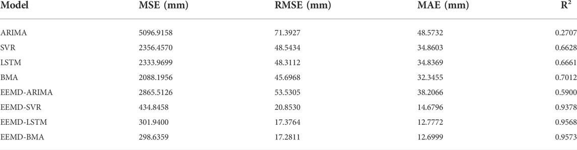
TABLE 4. Performances of different models.

We use CP and MW to measure the superiority of the BMA interval prediction, as shown in Table 5. The CP of the BMA is 87.5%, with some extreme precipitation events falling outside the 90% confidence interval. the MW of the BMA is 153.132 mm, which is too wide to provide valid information. The EEMD-BMA has a larger CP and a smaller MW, which suggests that the EEMD-BMA has a more appropriate prediction interval than the BMA and can provide more useful information for decision makers. For example, excessive precipitation during the rainy season may cause flooding and landslides, threatening people’s lives and property. The point prediction results may underestimate the actual precipitation, leading people to suffer losses due to under-preparedness. Decision makers can prepare in advance to reduce losses based on the upper limit of the confidence interval of the EEMD-BMA.

TABLE 5

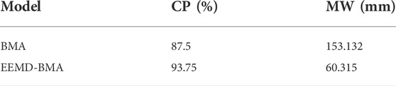
TABLE 5. Performances of BMA and EEMD-BMA.

3.5 Discussion

Since the monthly precipitation series have strong nonlinear fluctuations, it is difficult for a single model to identify the variation pattern of monthly precipitation. Therefore, the prediction performances of single models are poor. Both EEMD and BMA can improve the prediction accuracy of a single model, and EEMD improves more. BMA can provide confidence intervals of the prediction results to quantify uncertainty. the EEMD-BMA model combines the advantages of EEMD and BMA, and the prediction results have high accuracy and reliability. In other nonlinear time series forecasting problems, EEMD-BMA model also has some application value. It is worth noting that the prediction performance of EEMD-LSTM and EEMD-ARIMA models differ greatly, which affects the effect of BMA to some extent. The weight of EEMD-ARIMA model is very small, and its contribution to BMA is almost zero. Therefore, replacing the ARIMA model with more effective models may lead to better ensemble prediction results.

4 Conclusion

In this study, a hybrid EEMD-BMA model is proposed to predict the monthly precipitation data series. The main conclusions are as follows: 1) Processing precipitation data with the EEMD method can significantly improve the predictive power of the model. 2) We use the average of the reconstruction error as its predicted value and add it to the predictions of the components to obtain the final prediction of precipitation. In this way the accuracy of the precipitation prediction can be further improved. 3) BMA can take full advantage of the strengths of individual models to obtain more accurate results. Compared with other models, the EEMD-BMA model has optimal prediction performance. 4) The EEMD-BMA can quantify the uncertainty of the prediction results and give suitable confidence intervals. Based on the EEMD-BMA prediction results and confidence intervals, decision makers have more flexibility to develop effective measures against potential disasters.

In this paper, we only studied the effect of BMA on ensemble prediction. In future studies, other weighting methods, such as stacking and blending, can be tried for comparison with BMA.

Data availability statement

Publicly available datasets were analyzed in this study. This data can be found here: http://data.cma.cn.

Author contributions

Author contributions: conceptualization, SL and MLZ; data curation, MTZ, and XL; funding acquisition, MLZ; methodology, SL and YN; software, SL; visualization, SL and YN; writing“original draft preparation, SL; writing”review and editing, MLZ, XJ, and RC. All authors will be informed about each step of manuscript processing including submission, revision, revision reminder, etc. via emails from our system or assigned Assistant Editor.

Funding

This research was funded by the Key Research and Development Program of Gansu Province, China (21YF5WA096); the Young Tutor Support Fund Project of the Gansu Agriculture University (GAU-QDFC-2019-03); and the Natural Science Foundation of Gansu Province, China (1606RJZA077 and 1308RJZA262).

Acknowledgments

We thank Stephen Nazieh for his help in revising the language of this paper.

Conflict of interest

The authors declare that the research was conducted in the absence of any commercial or financial relationships that could be construed as a potential conflict of interest.

Publisher’s note

All claims expressed in this article are solely those of the authors and do not necessarily represent those of their affiliated organizations, or those of the publisher, the editors and the reviewers. Any product that may be evaluated in this article, or claim that may be made by its manufacturer, is not guaranteed or endorsed by the publisher.

References

Adebiyi, A. A., Adewumi, A. O., and Ayo, C. K. (2014). Comparison of ARIMA and artificial neural networks models for stock price prediction. J. Of Appl. Math. 2014, 1–7. doi:10.1155/2014/614342

CrossRef Full Text | Google Scholar

Al-Smadi, M., Talafha, B., Al-Ayyoub, M., and Jararweh, Y. (2019). Using long short-term memory deep neural networks for aspect-based sentiment analysis of Arabic reviews. Int. J. Of Mach. Learn. And Cybern. 10, 2163–2175. doi:10.1007/S13042-018-0799-4

CrossRef Full Text | Google Scholar

Belvederesi, C., Dominic, J. A., Hassan, Q. K., Gupta, A., and Achari, G. (2020). Predicting river flow using an ai-based sequential adaptive neuro-fuzzy inference system. Water 12 (6), 1622. doi:10.3390/W12061622

CrossRef Full Text | Google Scholar

Bengio, Y., Simard, P., and Frasconi, P. (1994). Learning long-term dependencies with gradient descent is difficult. IEEE Trans. Neural Netw. 5, 157–166. doi:10.1109/72.279181

PubMed Abstract | CrossRef Full Text | Google Scholar

Cheng, C. T., Niu, W. J., Feng, Z. K., Shen, J. J., and Chau, K. W. (2015). Daily reservoir runoff forecasting method using artificial neural network based on quantum-behaved particle swarm optimization. Water 7, 4232–4246. doi:10.3390/W7084232

CrossRef Full Text | Google Scholar

Ching, J., and Chen, Y. C. (2007). Transitional Markov chain Monte Carlo method for Bayesian model updating, model class selection, and model averaging. J. Eng. Mech. 133 (7), 816–832. doi:10.1061/(asce)0733-9399(2007)133:7(816)

CrossRef Full Text | Google Scholar

Draper, D. (1995). Assessment and propagation of model uncertainty. J. Of R. Stat. Soc. Ser. B Methodol. 57 (1), 45–70. doi:10.1111/J.2517-6161.1995.Tb02015.X

CrossRef Full Text | Google Scholar

Fischer, T., and Krauss, C. (2018). Deep learning with long short-term memory networks for financial market predictions. Eur. J. Of Operational Res. 270, 654–669. doi:10.1016/J.Ejor.2017.11.054

CrossRef Full Text | Google Scholar

Hochreiter, S., and Schmidhuber, J. (1997). Long short-term memory. Neural Comput. 9, 1735–1780. doi:10.1162/Neco.1997.9.8.1735

PubMed Abstract | CrossRef Full Text | Google Scholar

Huang, N. E., Shen, Z., Long, S. R., Wu, M. C., Shih, H. H., Zheng, Q., et al. (1998). The empirical mode decomposition and the hilbert spectrum for nonlinear and non-stationary time series analysis. Proc. Of R. Soc. Of Lond. Ser. A Math. Phys. And Eng. Sci. 454, 903–995. doi:10.1098/Rspa.1998.0193

CrossRef Full Text | Google Scholar

Jabbari, A., and Bae, D. H. (2018). Application of artificial neural networks for accuracy enhancements of real-time flood forecasting in the imjin basin. Water 10 (11), 1626. doi:10.3390/W10111626

CrossRef Full Text | Google Scholar

Jiang, S., Ren, L., Xu, C. Y., Liu, S., Yuan, F., Yang, X. L., et al. (2018). Quantifying multi-source uncertainties in multi-model predictions using the Bayesian model averaging scheme. Hydrology Res. 49, 954–970. doi:10.2166/Nh.2017.272

CrossRef Full Text | Google Scholar

Jimeno-Saez, P., Senent-Aparicio, J., Perez-Sanchez, J., Pulido-Velazquez, D., and Cecilia, J. M. (2017). Estimation of instantaneous peak flow using machine-learning models and empirical formula in peninsular Spain. Water 9 (5), 347. doi:10.3390/W9050347

CrossRef Full Text | Google Scholar

Kang, A. Q., Tan, Q. X., Yuan, X. H., Lei, X. H., and Yuan, Y. B. (2017). Short-term wind speed prediction using eemd-lssvm model. Adv. Meteorology, 1–22. doi:10.1155/2017/6856139

CrossRef Full Text | Google Scholar

Kang, J., Wang, H., Yuan, F., Wang, Z., Huang, J., Qiu, T., et al. (2020). Prediction of precipitation based on recurrent neural networks in jingdezhen, jiangxi province, China. Atmosphere 11 (3), 246. doi:10.3390/Atmos11030246

CrossRef Full Text | Google Scholar

Kratzert, F., Klotz, D., Brenner, C., Schulz, K., and Herrnegger, M. (2018). Rainfall-runoff modelling using long short-term memory (lstm) networks. Hydrol. Earth Syst. Sci. 22, 6005–6022. doi:10.5194/Hess-22-6005-2018

CrossRef Full Text | Google Scholar

Lai, Y. C., and Dzombak, D. A. (2020). Use of the autoregressive integrated moving average (ARIMA) model to forecast near-term regional temperature and precipitation. Weather Forecast. 35, 959–976. doi:10.1175/Waf-D-19-0158.1

CrossRef Full Text | Google Scholar

Li, J., Deng, D., Zhao, J., Cai, D., Hu, W., Zhang, M., et al. (2021). A novel hybrid short-term load forecasting method of smart grid using mlr and lstm neural network. IEEE Trans. Ind. Inf. 17, 2443–2452. doi:10.1109/Tii.2020.3000184

CrossRef Full Text | Google Scholar

Lippi, M., Montemurro, M. A., Degli Esposti, M., and Cristadoro, G. (2019). natural language statistical features of lstm-generated texts. IEEE Trans. Neural Netw. Learn. Syst. 30, 3326–3337. doi:10.1109/Tnnls.2019.2890970

PubMed Abstract | CrossRef Full Text | Google Scholar

Meira Neto, A. A., Oliveira, P. T. S., Rodrigues, D. B., and Wendland, E. (2018). Improving streamflow prediction using uncertainty analysis and Bayesian model averaging. J. Hydrol. Eng. 23 (5), 05018004. doi:10.1061/(Asce)He.1943-5584.0001639

CrossRef Full Text | Google Scholar

Pérez, C. J., Martín, J., and Rufo, M. J. (2006). Sensitivity estimations for Bayesian inference models solved by MCMC methods. Reliab. Eng. Syst. Saf. 91 (10-11), 1310–1314. doi:10.1016/J.Ress.2005.11.029

CrossRef Full Text | Google Scholar

Stephens, M. (2000). Bayesian analysis of mixture models with an unknown number of components-an alternative to reversible jump methods. Ann. Of Statistics 28, 40–74. doi:10.1214/aos/1016120364

CrossRef Full Text | Google Scholar

Sundermeyer, M., Ney, H., and Schluter, R. (2015). From feedforward to recurrent lstm neural networks for language modeling. IEEE/ACM Trans. Audio Speech Lang. Process. 23, 517–529. doi:10.1109/Taslp.2015.2400218

CrossRef Full Text | Google Scholar

Tayyab, M., Ahmad, I., Sun, N., Zhou, J. Z., and Dong, X. H. (2018). Application of integrated artificial neural networks based on decomposition methods to predict streamflow at upper Indus basin, Pakistan. Atmosphere 9 (12), 494. doi:10.3390/Atmos9120494

CrossRef Full Text | Google Scholar

Wang, D., Wang, C., Xiao, J., Xiao, Z., Chen, W., Havyarimana, V., et al. (2019). Bayesian optimization of support vector machine for regression prediction of short-term traffic flow. Intell. Data Anal. 23, 481–497. doi:10.3233/Ida-183832

CrossRef Full Text | Google Scholar

Wang, J., Wang, X., Lei, X. H., Wang, H., Zhang, X. H., You, J. J., et al. (2020). Teleconnection analysis of monthly streamflow using ensemble empirical mode decomposition. J. Of Hydrology 582, 124411. doi:10.1016/J.Jhydrol.2019.124411

CrossRef Full Text | Google Scholar

Wu, Z., and Huang, N. E. (2009). Ensemble empirical mode decomposition: A noise-assisted data analysis method. Adv. Adapt. Data Anal. 1, 1–41. doi:10.1142/S1793536909000047

CrossRef Full Text | Google Scholar

Xu, L., Chen, N., Zhang, X., and Chen, Z . (2020a). A data-driven multi-model ensemble for deterministic and probabilistic precipitation forecasting at seasonal scale. Clim. Dyn. 54 (7), 3355–3374. doi:10.1007/S00382-020-05173-X

CrossRef Full Text | Google Scholar

Xu, W., Jiang, Y. N., Zhang, X. L., Li, Y., Zhang, R., Fu, G. T., et al. (2020b). Using long short-term memory networks for river flow prediction. Hydrology Res. 51, 1358–1376. doi:10.2166/Nh.2020.026

CrossRef Full Text | Google Scholar

Yuan, R., Cai, S., Liao, W., Lei, X., Zhang, Y., Yin, Z., et al. (2021). Daily runoff forecasting using ensemble empirical mode decomposition and long short-term memory. Front. Earth Sci. (Lausanne). 9, 129. doi:10.3389/Feart.2021.621780

CrossRef Full Text | Google Scholar

Zeugner, S. (2011). Bayesian model averaging with bms. Tutorial to the R-package BMS. 1–30.

Google Scholar

Zhang, X., Zhang, Q., Zhang, G., Nie, Z., Gui, Z., Que, H., et al. (2018). A novel hybrid data-driven model for daily land surface temperature forecasting using long short-term memory neural network based on ensemble empirical mode decomposition. Int. J. Environ. Res. Public Health 15 (5), 1032. doi:10.3390/Ijerph15051032

PubMed Abstract | CrossRef Full Text | Google Scholar

Zhao, T., and Wang, Y. (2020). Non-parametric simulation of non-stationary non-Gaussian 3d random field samples directly from sparse measurements using signal decomposition and Markov chain Monte Carlo (mcmc) simulation. Reliab. Eng. Syst. Saf. 203, 107087. doi:10.1016/J.Ress.2020.107087

CrossRef Full Text | Google Scholar