The effects of tropical cyclones on characteristics of barrier layer thickness

Introduction

Tropical cyclones (TCs) are devastating weather systems that originate and develop over the warm ocean surface, with their energy coming mostly from sea-to-air enthalpy fluxes (Emanuel, 1986; Ma and Fei, 2022). Strong near-surface wind stress of TCs forces dramatic changes in the thermal and dynamic processes of the upper ocean, entraining cooler water from the thermocline to the surface of the ocean and decreasing the sea surface temperature (SST). The decreased SST leads to suppressed sea-to-air enthalpy fluxes, thereby playing a detrimental role in the intensification of TCs (Price, 1981; Bender et al., 1993; Bender and Ginis, 2000; Lloyd and Vecchi, 2011; Li et al., 2022). As such, the activities of TCs are highly sensitive to the ocean's response to TCs.

The extent of oceanic response has been traditionally regarded as a function of TC characteristics such as translation speed and intensity, and the upper ocean characteristics such as mixed-layer depth and thermocline gradient, wherein mesoscale oceanic eddies have played an important role (Liu et al., 2021; Ma et al., 2021). However, salinity is also a fundamental element of the oceanic environment. In the regions where there is plenty of fresh water input, a halocline may form within the isothermal layer, creating a barrier layer (BL) that acts as a barrier to vertical entrainment of cooler water beneath (Sprintall and Tomczak, 1992). Previous studies demonstrate that the BL can inhibit the TC-induced SST decrease due to its suppression of vertical mixing and entrainment cooling via increased stability (Wang et al., 2011; Neetu et al., 2012; Reul et al., 2014; Newinger and Toumi, 2015), with its effect depending on the characteristics of TCs and the ocean background (Yan et al., 2017; Rudzin et al., 2017). The BL impact on SST response can feedback to TC intensities effectively (Grodsky et al., 2012; Vissa et al., 2013; Mawren and Reason, 2017). Using a string of observations and coupled model simulations, Balaguru et al. (2012) proposed that the intensification rate of TCs can be ∼50% higher in regions with the BLs than in those without the BLs on a global scale.

Although there has been increasing literature about the role of BLs in TC-induced oceanic response and subsequent TC intensity evolutions, current knowledge of how the BL is modulated by TCs is limited. Using Argo float profiles in the Atlantic and central and eastern Pacific, Steffen and Bourassa, 2018 found that the BL characteristics can be changed effectively over the Atlantic and central Pacific basins but negligibly over the eastern Pacific basin after the passage of TCs. Their follow-up work on the case of Hurricane Gonzalo evinces that high precipitation rates in TCs could be a potential contributor to the BL strengthening (Steffen and Bourassa, 2020). Nonetheless, the limited sample sizes of Argo floats may hinder a more generalized investigation, especially the spatial and temporal changes in BL characteristics. It also matters whether the BL changes by TCs are perpetual or not. Therefore, this study aims to examine the impact of TCs on the spatial and temporal characteristics of BLs in the Northern Hemisphere, using a combination of Simple Ocean Data Assimilation reanalysis (SODA) data and Argo float data. A set of idealized experiments are carried out using the 3DPWP model to examine the mechanisms leading to the changes in BL thickness. The data and methodology are introduced in section 2. Section 3 presents the statistical results and Section 4 presents the simulation results, with a summary provided in section 5.

Data and methods

The TC information including center position, maximum surface wind, and translation speed is derived from the International Best Track Archive for Climate Stewardship (IBTrACS; Knapp et al., 2010). The SODA v3.12.2 reanalysis dataset (Mawren and Reason, 2017) at a temporal resolution of 5 days and spatial resolutions of 0.25 × 0.25° and Argo float profiles are used to obtain the BL characteristics. All Argo float profiles consist of delayed mode and quality-controlled data. Ocean temperatures are accurate to ±0.002°C, pressures to within ±2.4 dbar, and salinities to within ±0.01 PSU (Carval and Coauthors, 2011). A time period from 2002 to 2016 is chosen for the SODA dataset and Argo dataset.

The BL is defined to exist if the isothermal layer (IL) is thicker than the mixed layer (ML). Its thickness is calculated as the difference between the isothermal layer and the mixed layer following De Boyer Montégut et al., 2007:

$BLT = ILD – \mathit{M}\mathit{L}\mathit{D},(1)$

where BLT is barrier layer thickness, ILD is isothermal layer depth, and MLD is mixed layer depth. For the SODA and Argo dataset, MLD is defined as the depth where the density (ρ) had increased by 0.125 kg $m^{-3}$ when compared to surface density (${\rho }_0$; Girishkumar et al., 2014; Levitus, 1982; Ye et al., 2019). The ILD is calculated as the depth where the temperature has decreased by 0.5°C from a 5-m reference depth (Levitus, 1982; Bosc et al., 2009; Girishkumar et al., 2014; Ye et al., 2019). After conducting experiments using different criteria for calculating ILD and MLD, Steffen and Bourassa (2018) found that TC-induced changes to BL characteristics are qualitatively consistent regardless of the threshold criteria selected.

The research area of this study is the region with frequent tropical cyclone activities in the northern hemisphere (0–40°N). Similar to Ma et al. (2020), we define a square domain with widths of 20° along and across the TC track at spatial resolutions of 0.1° × 0.1°, centered on the TC center for each best-track data point (Ma et al., 2018). The x axis of a domain is across the TC track and the y axis is along the TC track. A total of 50339 domains are identified by best track data points. The ILD, MLD, and BLT obtained from SODA data are bilinear- interpolated and rotated into the domain according to the TC translation direction. For each domain, a 101-days time period from −10 to 90 days relative to TC passage is calculated for each variable (ILD, MLD, and BLT). The anomalies of these variables are all calculated by the post-storm value minus the pre-storm value, wherein the pre-storm value is defined as an average between −10 and −5 days relative to TC passage (Ma et al., 2020). In order to better understand the evolution of BLT, and consolidate the observed results of SODA data, we select the Argo float profiles within 200 km around the TC recording point according to the time change, screened out the data with incomplete data or errors, and verify the results obtained from SODA data. These two observational datasets are combined by considering that the Argo dataset is relatively precise but cannot provide complete spatial and temporal characteristics; the SODA data are not so accurate but can capture the whole spatial and temporal evolution of BL characteristics.

Numerical simulations were performed using the three-dimensional Price–Weller–Pinkel (3DPWP) ocean model. The 3DPWP model initiates the mixing of the water column when critical bulk and gradient Richardson number criteria are met. Specific details of the model’s physics are found in Price et al. (1986) and Price et al. (1994). A modification is made by changing the mixed layer definition following the observational analysis so that the simulation results can be largely consistent with the observational results. All simulations were performed using a fixed domain on an f plane at 22°N with a horizontal grid spacing of 5 km and with 200 × 200 grid points in the zonal and meridional directions. The time step was set to 60 s, and each simulation was integrated for 30 days with the output being saved every 6 h. The model was composed of 45 vertical levels separated by Δz of 5 m from the first model level of 2.5 m down to 97.5 m, Δz of 10 m from the level of 97.5 m down to 197.5 m, and Δz of 50 m below that to a depth of 947.5 m. According to the criteria used in SODA and ARGO data to judge ILD and MLD, we set a temperature and salinity profile with the presence of BL at the initial time. This setting is to simulate the process of BL erosion after TC came, and can also reflect the influence of precipitation on BL generation. The MLD is 20.8 m, and the ILD is 55 m, thus the BLT is 34.2 m. The wind field used in the model to simulate TC is a classic Rankine vortex structure with the maximum wind speed being set to 60 m $s^{-1}$ and its translation speed being set to 5 m $s^{-1}$. The sensitivity of BLT, ILD, and MLD to precipitation is also discussed by changing the total precipitation in this study.

Statistical results

Figure 1 shows the temporal evolution of the along-track averaged composite BLT anomaly. The climatological trend of BL is calculated first and then removed from the BLT anomaly. A remarkably positive BLT anomaly is formed accompanying the TC’s arrival, with the increase reaching up to ∼1.31 m (26.93%) relative to the pre-storm state. The deepening of the BL caused by TCs is consistent with previous studies (Fu et al., 2014; Steffen and Bourassa, 2018, 2020). With the thickening of ILD and the shallowing of MLD, the increase in BLT reaches its maximum 1–5 days after TC arrival and recovers to the pre-storm status rapidly in 30 days (Figure 1B), with small fluctuations in the following 30–90 days. This result suggests that TCs cause statistically significant changes in BLT, which, however, are not perpetual features. After the passage of TCs, the BL recovers to its pre-storm status rapidly and it seems that the correlation between this recovery process and TC characteristics is weak (Figure 2). The behaviors of BLT indicate that if a subsequent TC overlaps with the track of a prior one in the TC season, cyclone-to-cyclone interaction may occur via the path of BLT; however, the TC-induced BL changes cannot have a profound influence on TCs in the coming year. As can be seen from the right part of Figure 1A, the maximum value of the BLT anomaly appears at the left position of the TC track, while the BLT thickening is slightly rightward biased on the whole (within 5° from the TC path). This feature is similar to the responses of SST and mixed layer current (Price, 1981; Qiu et al., 2019).

FIGURE 1

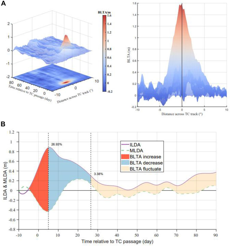
FIGURE 1. Temporal evolution of the along-track-averaged composite (A) barrier layer thickness anomaly (m) and (B) average value of BLT change within 200 km across TC track. The climatological trend has been removed from the anomalies of barrier layer thickness. The two black-dashed lines in (B) denote the largest and smallest proportion of barrier layer thickness anomaly (BLTA) before TC came respectively. Different colored areas in (B) represent different stages in which barrier layer thickness changes. The purple line represents the change of isothermal layer anomaly (ILDA). The green dashed line denotes the evolution of mixed layer anomaly (MLDA).

FIGURE 2

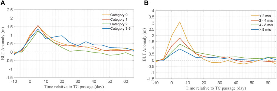
FIGURE 2. The recovery process of BLT anomaly under different TC categories (A) and under different TC translation speeds (B) in 65 days. Category 0–5 refers to a tropical depression, tropical storm, severe tropical storm, typhoon, severe typhoon, and super typhoon, respectively (same as Figures 3, 7).

The intensity and translation speed are two of the most fundamental characteristics of TCs. Figure 3 shows the maximum value of the BLT anomaly as a function of TC intensity categories and translation speeds. Overall the discrepancies of BLT anomalies reveal a significant dependence on both the intensity and translation speed of TCs. The TC-induced changes in BLT tend to be larger as the storm is stronger or moves slower (Figures 4, 5). The occurrence of BLT anomaly is closely related to two aspects: one is upper-ocean turbulent mixing and the ILD deepening due to TC wind stress forcing, and another one is the MLD shoaling due to the input of a large amount of freshwater flux which will also be reflected in the analysis of simulation results later. In the inner core of a TC, the net freshwater fluxes of strong or slow TCs are much more effective than those under the weak or fast TCs (Fu et al., 2014). Moreover, slow-moving TCs can accumulate higher precipitation totals over the ocean (Steffen and Bourassa, 2018), and thus the BLT will develop more rapidly by stronger or slower TCs. When the freshwater input becomes less, the wind force weakens and the TC vertical mixing becomes weaker, and hence the development of the barrier layer is also blocked.

FIGURE 3

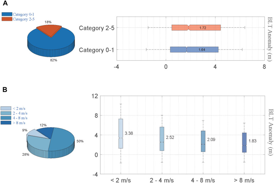
FIGURE 3. The pie charts (left) in (A) and (B) show the percentage of sample size under different TC characteristics (total sample size: 50339). The boxplots (right) in (A) and (B) represent the relationship between the BLT anomaly and TC intensity as well as its translation speed, respectively. The numbers in the figure represent the size of the 50th percentile. The difference between the two adjacent groups is statistically significant above the 99% confidence level based on the Student’s t-test.

FIGURE 4

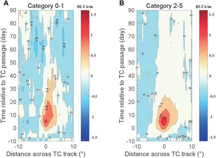
FIGURE 4. The temporal evolution of the along-track-averaged composite barrier layer thickness anomaly (m) under different TC categories.

FIGURE 5

FIGURE 5. The temporal evolution of the along-track-averaged composite barrier layer thickness anomaly (m) under different TC translation speeds.

The change of ILD forced by TC is significant (Figure 6A). An abnormal thickening appears on both sides of the TC path, and the thickening on the right side is obviously stronger than that on the other, while the recovery of thickening on the left side seems to be more quickly. The asymmetric distribution of ILD anomalies on both sides of the TC track leads to a certain right-biased trend of BLT anomalies. Actually, under the strong disturbance of TC, the MLD also has an obvious thickening phenomenon on both sides of the TC path. However, unlike the change of ILD, MLD becomes shallower on the left side of the TC path (Figure 6B) due to the precipitation caused by TC. The input of a large amount of freshwater makes the salinity of the upper ocean desalinate, the density decreases correspondingly, and the stability of the upper ocean increases (Fu et al., 2014; Steffen and Bourassa, 2018; Zhang et al., 2021). This explains why the maximum value of the BLT anomaly appears on the left side of the TC path. As is shown in Figure 6A, the rightward bias of isothermal layer deepening is more evident in Figure 7B. In the range of 150–300 km to the right of the TC track (Figure 7B), the anomaly of ILD is significantly higher than that near the area of the TC center, which may be to some extent related to the stronger left-right asymmetry distribution of the wind stress of TCs (Fu et al., 2014). Compared with the left side, the strong wind stress on the right side of the TC center plays a leading role in stirring the ocean surface. Consequently, the effect of vertical mixing which is crucial to the deepening of the IL and is confined to the right of the TC track (Zhang et al., 2016) becomes dominant compared to the upwelling effect that has a certain influence on the uplift of the IL. The influence of the heat pump effect (Emanuel, 2001; Korty et al., 2008; Pasquero and Emanuel, 2008; Fedorov et al., 2010) and the cold suction effect (Bueti et al., 2014; Price, 1981; Vincent et al., 2012) corresponding to vertical mixing and upwelling, respectively, on the structure of the upper-ocean is reflected in the changes of the IL.

FIGURE 6

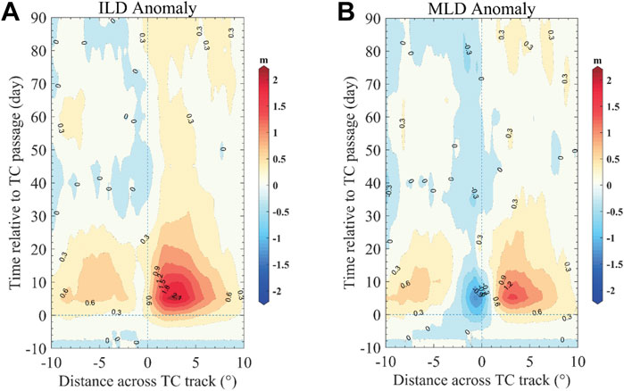
FIGURE 6. Temporal evolution of the along-track-averaged composite (A) isothermal layer depth (m) and (B) mixed layer depth (m). The climatological trend has been removed from the anomalies of isothermal layer depth and mixed layer depth.

FIGURE 7

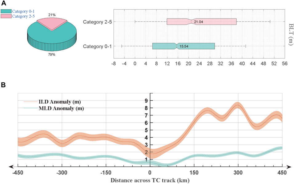
FIGURE 7. The pie chart (left) in (A) shows the percentage of Argo profile size within 200 km around the best track recording point (total profile size: 2801). The boxplot (right) in (A) represents the relationship between the BLT and the intensity of TCs. The difference between the two adjacent groups is statistically significant above the 99% confidence level based on the Student’s t-test. The changes of ILD anomaly(red) and MLD anomaly (green) by Argo data within 450 km across the TC track are shown in (B). The result in the figure is calculated by subtracting the average value of 5–7 days before TC came from the average value within 10 days after TC left. The solid line in the (B) represents the average value and the shaded areas represent standard errors which are calculated as the standard deviation divided by the square root of each sample size.

Using Argo data, the relationship between BL changes and TC Intensity is also been analyzed (Figure 7A). Compared with weak TCs, the changes in BLT caused by strong TCs is more obvious. From the results (Figure 8) of 7 days, before TC came to 21 days after it left, BLT, ILD, and MLD all experienced the process of thickening first under the force of TC and then gradually recovering. The difference is that MLD thickened and recovered faster and became shallower. All the results are consistent with the conclusion obtained by using SODA data.

FIGURE 8

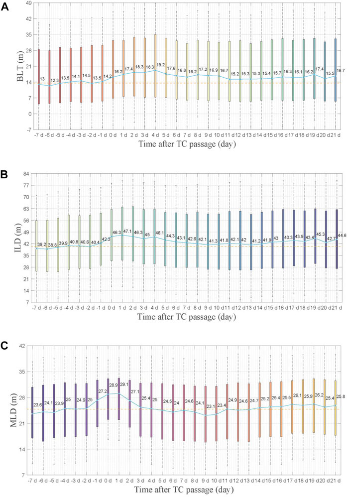
FIGURE 8. (A), (B), and (C) use Argo data to show the boxplot of BLT, ILD, and MLD changes from 7 days before TC came to 21 days after TC left. The blue lines and the numbers in the figure represent the size of the 50th percentile. The yellow dotted lines indicate the median mean value of the 7 days before TC came.

The spatial distribution of the BLT anomaly is closely related to the areas with frequent TC activities (Figure 9). In coastal regions, as well as in the equatorial low latitudes of the Pacific and Atlantic Oceans, the Bay of Bengal, and parts of the Arabian Sea, the BLT anomaly has obvious positive values. These areas are not only with frequent TC activities, but also the regions where BL appears (Agarwal et al., 2012; Mignot et al., 2012; Echols and Riser, 2020). In these regions, BL and TC interact with each other frequently, and therefore should be paid more attention.

FIGURE 9

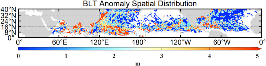
FIGURE 9. Spatial distribution of BLT anomaly in each 1° × 1° bin over the Northern Hemisphere by SODA data.

Simulation results

High precipitation rates within TCs can provide a large freshwater flux to the surface that alters upper-ocean stratification and thus can act as a potential mechanism to strengthen the BL. In order to explore the effect of precipitation on the changes of BLT, ILD, and MLD, we carried out a series of ideal numerical experiments using the 3DPWP model. The setting of the temperature profile at the initial time (Figure 10A) is common in equatorial subtropical waters and is conducive to the formation and development of TC. For salinity, we constructed a profile with low surface salinity and a relatively shallow depth of mixed layer, and hence there is a thick BL between the shallower ML and the deeper IL. The translation speed of the simulated typhoon is 5 $m s^{-1}$ and it reached the center of the grid in the 30th hour of the simulation. The preexisting BL was rapidly eroded and disappeared (Figure 11) shortly after the TC reached, and the deeper IL signal also disappeared (Figure 12) under the influence of the stronger upwelling in the center of the TC (not shown). The initial setting of the MLD is shallow relative to the upwelling process induced by the TC, which reaches a depth of ∼200 m. ML is not markedly affected at the center of TC due to weak winds and precipitation there. Under the disturbance of TC strong wind stress and precipitation, the vertical mixing of the upper ocean dominates, ILD and MLD show obvious thickening (Figure 13) on both sides of the TC path, and the thickening on the right side of ILD is greater than that on the left, which is consistent with the results obtained from Argo and SODA data. BLT showed a thickening process under the combined action of ILD and MLD too, and the thickening on the right side was significantly larger than that on the left.

FIGURE 10

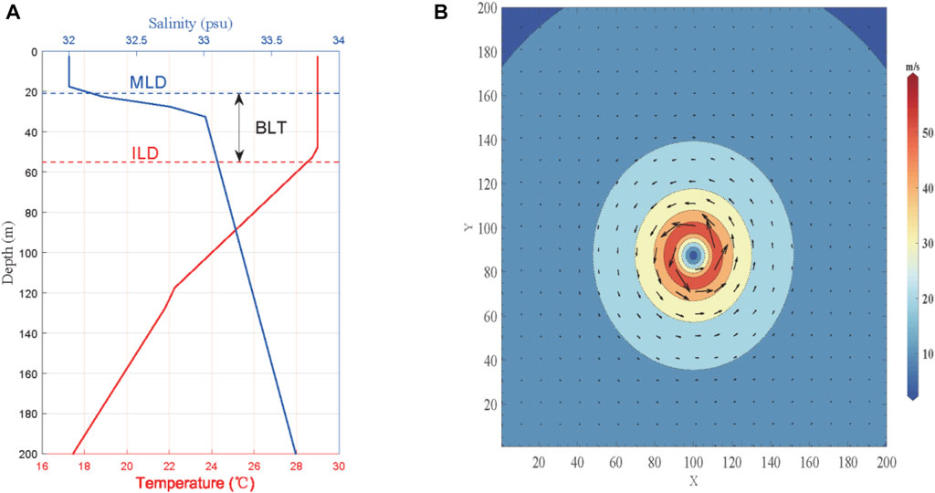
FIGURE 10. (A) Temperature (°C) and salinity (psu) profiles used in 3DPWP simulations. The blue and red dashed lines represent MLD and ILD respectively. (B) vector wind field used in the simulation, with color shading for wind speed.

FIGURE 11

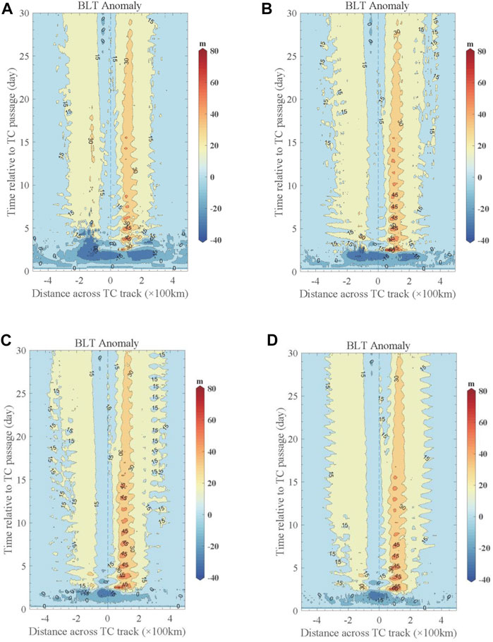
FIGURE 11. (A–D) show the results of BLT anomaly within 30 days of simulation under the conditions of normal, 2 times, 5 times, and 10 times precipitation.

FIGURE 12

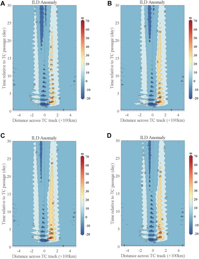
FIGURE 12. (A–D) show the results of ILD anomaly within 30 days of simulation under the conditions of normal, 2 times, 5 times, and 10 times precipitation.

FIGURE 13

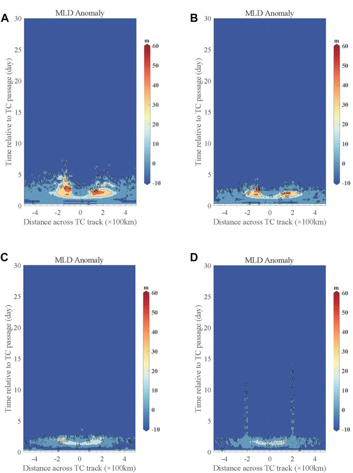
FIGURE 13. (A–D) show the results of MLD anomaly within 30 days of simulation under the conditions of normal, 2 times, 5 times, and 10 times precipitation.

In the sensitivity test to precipitation (Figures 11–13), the variation of MLD is obviously larger than that of BLT and MLD. In a case study using the ROMS model, Steffen and Bourassa (2020) found that the precipitation forcing has a large transformation on the MLD, while the ILD is almost unaffected. Figures 13B–D show the changes of MLD anomaly under different intensities of precipitation. As the total amount of precipitation increases, the positive anomalous signal of MLD gradually weakens and returns to the level pre-TC in a short time after TC departure. Under the force of a large amount of freshwater on the surface, MLD shows a negative abnormal state within 20 days after TC’s departure. In contrast to the MLD, the ILD appears to be not sensitive to the amount of precipitation. Even in the case of extreme precipitation, the change of the ILD anomaly signal remains weak. All four precipitation forcing conditions in the simulation promote the generation of BL and it shows the phenomenon of being eroded and regenerated, but the generated BL seems to be insensitive to the precipitation under extreme conditions, and the change of abnormal signals of BLT is mainly manifested in the eroded stage.

Conclusion and discussion

The interaction between BL and TCs has attracted increasing attention in recent years. Previous studies have found a significant role of the BL in modulating the TC-induced oceanic response as well as their feedback on the intensities of TCs (Wang et al., 2011; Balaguru et al., 2012; Grodsky et al., 2012; Neetu et al., 2012; Vissa et al., 2013; Reul et al., 2014; Androulidakis et al., 2016; Rudzin et al., 2017; Yan et al., 2017; Qiu et al., 2019). However, current knowledge of how the spatial and temporal characteristics of BLs are determined by TCs is still limited. In this study, we investigate the TC-induced changes in BL characteristics in combination with SODA reanalysis data and observed Argo float profiles. We systematically quantify the evolution of BL forced by TCs and present its recovery process after TC departure from a statistical point of view. In addition, we conduct a series of ideal experiments using the 3DPWP ocean model for the sensitivity of BL to precipitation.

Results show that the BLT increases remarkably after TC passage, with the peak change being rightward biased slightly and reaching ∼1.31 m (26.93%) 1–5 days after TC arrival. This suggests that the BL is modulated by TCs effectively from a statistical viewpoint. However, the changes in BL characteristics are temporary features. After reaching its peak values, the BLT recovers to its pre-storm status within 30 days on average. The changes in BLT are also related to TC intensity and translation speed, with stronger or slower TCs corresponding to a larger BLT increase. The spatial distribution of BLT anomaly is closely related to the areas with frequent TC activities, mainly concentrated in coastal and equatorial low latitude areas.

The co-variation of MLD and ILD contributes to the change of BLT. Under the influence of precipitation brought by TCs, the development of BL shows a certain rightward deviation trend due to the input of a large number of freshwater fluxes on the surface of the upper ocean. The ILD is deepened with a rightward-biased asymmetry due to the forcing of TC wind.

Idealized experiments with the 3DPWP model reveal that the BL is eroded by TC and then generated under the influence of precipitation forcing. The apparent thickening of the ILD on the right side of the TC path and a certain right-biased trend of the BLT are well simulated. At the same time, it can be seen from the sensitivity of MLD to precipitation that the importance of freshwater input to the stability of the upper ocean and the development and formation of BL.

This study stresses the significant effect of TCs on modulating the BL characteristics, which is nonetheless a temporary change that lasts 1 month or so. Future work may extend to explore physical mechanisms leading to the spatial and temporal changes in BL features based on coupled numerical simulations. It may also be worth further studies on whether the changes in BL will have notable impacts on subsequent TCs sharing similar tracks in a relatively short period of time.

Data availability statement

The original contributions presented in the study are included in the article/Supplementary Material, further inquiries can be directed to the corresponding author.

Author contributions

ZZ: Mainly complete data download, interpolation processing, drawing analysis, paper writing. ZM: Scientific research ideas guidance and thesis revision.

Funding

This study is supported by Southern Marine Science and Engineering Guangdong Laboratory (Zhuhai) (No. SML2021SP207), the Program of Shanghai Academic/Technology Research Leader (21XD1404500), the National Natural Science Foundation of China (42022033, 42192552, and 41875062), and the Natural Science Foundation of Hunan Province, China (2020JJ3040).

Conflict of interest

The authors declare that the research was conducted in the absence of any commercial or financial relationships that could be construed as a potential conflict of interest.

Publisher’s note

All claims expressed in this article are solely those of the authors and do not necessarily represent those of their affiliated organizations, or those of the publisher, the editors, and the reviewers. Any product that may be evaluated in this article, or claim that may be made by its manufacturer, is not guaranteed or endorsed by the publisher.

References

Agarwal, N., Sharma, R., Parekh, A., Basu, S., Sarkar, A., Agarwal, V. K., et al. (2012). Argo observations of barrier layer in the tropical Indian Ocean. Adv. Space Res. 50 (5), 642–654. doi:10.1016/j.asr.2012.05.021

CrossRef Full Text | Google Scholar

Androulidakis, Y., Kourafalou, V., Halliwell, G., Le Hénaff, M., Kang, H., Mehari, M., et al. (2016). Hurricane interaction with the upper ocean in the Amazon-Orinoco plume region. Ocean. Dyn. 66 (12), 1559–1588. doi:10.1007/s10236-016-0997-0

CrossRef Full Text | Google Scholar

Balaguru, K., Chang, P., Saravanan, R., Leung, L. R., Xu, Z., Li, M., et al. (2012). Ocean barrier layers’ effect on tropical cyclone intensification. Proc. Natl. Acad. Sci. U. S. A. 109 (36), 14343–14347. doi:10.1073/pnas.1201364109

PubMed Abstract | CrossRef Full Text | Google Scholar

Bender, M. A., Ginis, I., and Kurihara, Y. (1993). Numerical simulations of tropical cyclone-ocean interaction with a high resolution coupled model. J. Geophys. Res. 98, 23 245–23 263. doi:10.1029/93jd02370

CrossRef Full Text | Google Scholar

Bender, M. A., and Ginis, I. (2000). Real case simulations of hurricane-ocean interaction using a high resolution coupled model: Effects on hurricane intensity. Mon. Weather Rev. 128, 917–946. doi:10.1175/1520-0493(2000)128<0917:rcsoho>2.0.co;2

CrossRef Full Text | Google Scholar

Bosc, C., Delcroix, T., and Maes, C. (2009). Barrier layer variability in the Western Pacific warm pool from 2000 to 2007. J. Geophys. Res. 114 (C6), C06023. doi:10.1029/2008JC005187

CrossRef Full Text | Google Scholar

Bueti, M. R., Ginis, I., Rothstein, L. M., and Griffies, S. M. (2014). Tropical cyclone–induced thermocline warming and its regional and global impacts. J. Clim. 27 (18), 6978–6999. doi:10.1175/jcli-d-14-00152.1

CrossRef Full Text | Google Scholar

Carval, T., and Coauthors, (2011). Argo user’s manual V3.2. IFREMER, 124. doi:10.13155/29825

CrossRef Full Text | Google Scholar

De Boyer Montégut, C., Mignot, J., Lazar, A., and Cravatte, S. (2007). Control of salinity on the mixed layer depth in the world ocean: 1. General description. J. Geophys. Res. 112 (C6), C06011. doi:10.1029/2006JC003953

CrossRef Full Text | Google Scholar

Echols, R., and Riser, S. C. (2020). Spice and barrier layers: an Arabian sea case study. J. Phys. Oceanogr. 50 (3), 695–714. doi:10.1175/jpo-d-19-0215.1

CrossRef Full Text | Google Scholar

Emanuel, K. A. (1986). An air-sea interaction theory for tropical cyclones. Part I: steady-state maintenance. J. Atmos. Sci. 43 (6), 585–605. doi:10.1175/1520-0469(1986)043<0585:aasitf>2.0.co;2

CrossRef Full Text | Google Scholar

Emanuel, K. (2001). Contribution of tropical cyclones to meridional heat transport by the oceans. J. Geophys. Res. 106 (D14), 14771–14781. doi:10.1029/2000jd900641

CrossRef Full Text | Google Scholar

Fedorov, A. V., Brierley, C. M., and Emanuel, K. (2010). Tropical cyclones and permanent el nino in the early Pliocene epoch. Nature 463 (7284), 1066–1070. doi:10.1038/nature08831

PubMed Abstract | CrossRef Full Text | Google Scholar

Fu, H., Wang, X., Chu, P. C., Zhang, X., Han, G., Li, W., et al. (2014). Tropical cyclone footprint in the ocean mixed layer observed by argo in the northwest Pacific. J. Geophys. Res. Oceans 119 (11), 8078–8092. doi:10.1002/2014jc010316

CrossRef Full Text | Google Scholar

Girishkumar, M. S., Suprit, K., Chiranjivi, J., Udaya Bhaskar, T. V. S., Ravichandran, M., Shesu, R. V., et al. (2014). Observed oceanic response to tropical cyclone Jal from a moored buoy in the south-Western Bay of Bengal. Ocean. Dyn. 64 (3), 325–335. doi:10.1007/s10236-014-0689-6

CrossRef Full Text | Google Scholar

Grodsky, S. A., Reul, N., Lagerloef, G., Reverdin, G., Carton, J. A., Chapron, B., et al. (2012). Haline hurricane wake in the amazon-orinoco plume: AQUARIUS/SACD and SMOS observations. Geophys. Res. Lett. 39 (20), 2012GL053335. doi:10.1029/2012GL053335

CrossRef Full Text | Google Scholar

Knapp, K. R., Kruk, M. C., Levinson, D. H., Diamond, H. J., and Neumann, C. J. (2010). The international best track archive for climate stewardship (IBTrACS). Bull. Am. Meteorol. Soc. 91 (3), 363–376. doi:10.1175/2009bams2755.1

CrossRef Full Text | Google Scholar

Korty, R. L., Emanuel, K. A., and Scott, J. R. (2008). Tropical cyclone–induced upper-ocean mixing and climate: Application to equable climates. J. Clim. 21 (4), 638–654. doi:10.1175/2007jcli1659.1

CrossRef Full Text | Google Scholar

Levitus, S. (1982). “Climatological atlas of the world ocean,” in NOAA prof. Pap. (Washington, DC: U.S. Govt. Printing Off), 13, 173.

Google Scholar

Li, X., Cheng, X., Fei, J., Huang, X., and Ding, J. (20222018). The modulation effect of sea surface cooling on the eyewall replacement cycle in typhoon trami. Mon. Weather Rev. doi:10.1175/MWR-D-21-0177.1

CrossRef Full Text | Google Scholar

Liu, Y., Lu, H., Zhang, H., Cui, Y., and Xing, X. (2021). Effects of ocean eddies on the tropical storm Roanu intensity in the Bay of Bengal. PLoS One 16 (3), e0247521. doi:10.1371/journal.pone.0247521

PubMed Abstract | CrossRef Full Text | Google Scholar

Lloyd, I. D., and Vecchi, G. A. (2011). Observational evidence for oceanic controls on hurricane intensity. J. Clim. 24 (4), 1138–1153. doi:10.1175/2010jcli3763.1

CrossRef Full Text | Google Scholar

Ma, Z., and Fei, J. (2022). A comparison between moist and dry tropical cyclones: The low effectiveness of surface sensible heat flux in storm intensification. J. Atmos. Sci. 79. doi:10.1175/JAS-D-21-0014.1

CrossRef Full Text | Google Scholar

Ma, Z., Fei, J., Huang, X., and Cheng, X. (2018). Modulating effects of mesoscale oceanic eddies on sea surface temperature response to tropical cyclones over the Western north Pacific. J. Geophys. Res. Atmos. 123 (1), 367–379. doi:10.1002/2017jd027806

CrossRef Full Text | Google Scholar

Ma, Z., Fei, J., Lin, Y., and Huang, X. (2020). Modulation of clouds and rainfall by tropical cyclone's cold wakes. Geophys. Res. Lett. 47 (17). doi:10.1029/2020GL088873

CrossRef Full Text | Google Scholar

Ma, Z. H., Zhang, Z. L., Fei, J. F., and Wang, H. Z. (2021). Imprints of tropical cyclones on structural characteristics of mesoscale oceanic eddies over the Western north Pacific. Geophys. Res. Lett. 48 (10). doi:10.1029/2021GL092601

CrossRef Full Text | Google Scholar

Mawren, D., and Reason, C. J. C. (2017). Variability of upper-ocean characteristics and tropical cyclones in the South West Indian Ocean. J. Geophys. Res. Oceans 122, 2012–2028. doi:10.1002/2016jc012028

CrossRef Full Text | Google Scholar

Mignot, J., Lazar, A., and Lacarra, M. (2012). On the formation of barrier layers and associated vertical temperature inversions: a focus on the northwestern tropical atlantic. J. Geophys. Res. 117, C02010. doi:10.1029/2011JC007435

CrossRef Full Text | Google Scholar

Neetu, S., Lengaigne, M., Vincent, E. M., Vialard, J., Madec, G., Samson, G., et al. (2012). Influence of upper-ocean stratification on tropical cyclone-induced surface cooling in the Bay of Bengal. J. Geophys. Res. 117 (C12). doi:10.1029/2012JC008433

CrossRef Full Text | Google Scholar

Newinger, C., and Toumi, R. (2015). Potential impact of the colored amazon and orinoco plume on tropical cyclone intensity. J. Geophys. Res. Oceans 120 (2), 1296–1317. doi:10.1002/2014jc010533

CrossRef Full Text | Google Scholar

Pasquero, C., and Emanuel, K. (2008). Tropical cyclones and transient upper-ocean warming. J. Clim. 21 (1), 149–162. doi:10.1175/2007jcli1550.1

CrossRef Full Text | Google Scholar

Price, J. F., Sanford, T., and Forristall, G. (1994). Forced stage response to amovinghurricane. J. Phys. Oceanogr. 24, 233–260. doi:10.1175/1520-0485(1994)024<0233:fsrtam>2.0.co;2

CrossRef Full Text | Google Scholar

Price, J. F. (1981). Upper ocean response to a hurricane. J. Phys. Oceanogr. 11, 153–175. doi:10.1175/1520-0485(1981)011<0153:uortah>2.0.co;2

CrossRef Full Text | Google Scholar

Price, J. F., Weller, R. A., and Pinkel, R. (1986). Diurnal cycling: Observations and models of the upper ocean response to diurnal heating, cooling, and wind mixing. J. Geophys. Res. 91 (C7), 8411. doi:10.1029/jc091ic07p08411

CrossRef Full Text | Google Scholar

Qiu, Y., Han, W., Lin, X., West, B. J., Li, Y., Xing, W., et al. (2019). Upper-ocean response to the super tropical cyclone Phailin (2013) over the freshwater region of the Bay of Bengal. J. Phys. Oceanogr. 49 (5), 1201–1228. doi:10.1175/jpo-d-18-0228.1

CrossRef Full Text | Google Scholar

Reul, N., Quilfen, Y., Chapron, B., Fournier, S., Kudryavtsev, V., Sabia, R., et al. (2014). Multisensor observations of the amazon-orinoco river plume interactions with hurricanes. J. Geophys. Res. Oceans 119 (12), 8271–8295. doi:10.1002/2014jc010107

CrossRef Full Text | Google Scholar

Rudzin, J. E., Shay, L. K., Jaimes, B., and Brewster, J. K. (2017). Upper ocean observations in eastern Caribbean Sea reveal barrier layer within a warm core eddy. J. Geophys. Res. Oceans 122 (2), 1057–1071. doi:10.1002/2016jc012339

CrossRef Full Text | Google Scholar

Sprintall, J., and Tomczak, M. (1992). Evidence of the barrier layer in the surface layer of the tropics. J. Geophys. Res. 97 (C5), 7305. doi:10.1029/92jc00407

CrossRef Full Text | Google Scholar

Steffen, J., and Bourassa, M. (2018). Barrier layer development local to tropical cyclones based on Argo float observations. J. Phys. Oceanogr. 48 (9), 1951–1968. doi:10.1175/jpo-d-17-0262.1

CrossRef Full Text | Google Scholar

Steffen, J., and Bourassa, M. (2020). Upper-ocean response to precipitation forcing in an ocean model hindcast of hurricane Gonzalo. J. Phys. Oceanogr. 50 (11), 3219–3234. doi:10.1175/jpo-d-19-0277.1

CrossRef Full Text | Google Scholar

Vincent, E. M., Madec, G., Lengaigne, M., Vialard, J., and Koch-Larrouy, A. (20122019–2038). Influence of tropical cyclones on sea surface temperature seasonal cycle and ocean heat transport. Clim. Dyn. 41 (7-8), 2019–2038. doi:10.1007/s00382-012-1556-0

PubMed Abstract | CrossRef Full Text | Google Scholar

Vissa, N. K., Satyanarayana, A. N. V., and Kumar, B. P. (2013). Response of upper ocean and impact of barrier layer on Sidr cyclone induced sea surface cooling. Ocean. Sci. J. 48 (3), 279–288. doi:10.1007/s12601-013-0026-x

CrossRef Full Text | Google Scholar

Wang, X., Han, G., Qi, Y., and Li, W. (2011). Impact of barrier layer on typhoon-induced sea surface cooling. Dyn. Atmos. Oceans 52 (3), 367–385. doi:10.1016/j.dynatmoce.2011.05.002

CrossRef Full Text | Google Scholar

Yan, Y., Li, L., and Wang, C. (2017). The effects of oceanic barrier layer on the upper ocean response to tropical cyclones. J. Geophys. Res. Oceans 122, 4829–4844. doi:10.1002/2017jc012694

CrossRef Full Text | Google Scholar

Ye, H., Sheng, J., Tang, D., Morozov, E., Kalhoro, M. A., Wang, S., et al. (2019). Examining the impact of tropical cyclones on air‐sea CO2 exchanges in the Bay of Bengal based on satellite data and in situ observations. J. Geophys. Res. Oceans 124 (1), 555–576. doi:10.1029/2018jc014533

CrossRef Full Text | Google Scholar

Zhang, H., Chen, D., Zhou, L., Liu, X., Ding, T., Zhou, B., et al. (2016). Upper ocean response to typhoon kalmaegi (2014). J. Geophys. Res. Oceans 121 (8), 6520–6535. doi:10.1002/2016jc012064

CrossRef Full Text | Google Scholar

Zhang, J., Lin, Y., and Ma, Z. (2021). Footprint of tropical cyclone cold wakes on top-of-atmosphere radiation. Geophys. Res. Lett. 48 (19). doi:10.1029/2021GL094705

CrossRef Full Text | Google Scholar