Properties and biases of the global heat flow compilation

1 Introduction

Studies of geothermal heat provide essential insight into the internal structure and history of the Earth (Kelvin, 1863; Pollack and Chapman, 1977; Beardsmore and Cull, 2001; Artemieva, 2011; Davies, 2013; Hasterok, 2013; Jaupart et al., 2016; Podugu et al., 2017; Lucazeau, 2019). A range of mechanisms control the amount of heat observed: thermal properties of the upper mantle, ongoing or recent tectonism (e.g. Pasquale et al., 2014; Goes et al., 2020), crustal heat production (e.g. Jaupart et al., 2016; Hasterok et al., 2018), topographic focusing by refraction (e.g. Lees et al., 1910), erosion and sedimentation (e.g. Von Herzen and Uyeda, 1963; Fukahata and Matsu’ura, 2001), advection by groundwater (e.g. Mansure and Reiter, 1979), and preserved variations and anomalies of paleoclimatic conditions (e.g. Huang et al., 1997; Šafanda et al., 2004).

Insights from geothermal measurements are applied in mineral prospecting (e.g. Cull et al., 1988), and hydrocarbon exploration, for example, to constrain the oil and gas windows (e.g. Royden and Sclater, 1980; Shalaby et al., 2011), and geothermal energy (Dickson and Fanelli, 2013). One particular aspect of geothermal heat flow that has recently gained attention is the impact of heat transfer at the base of ice sheets in Greenland and Antarctica (Burton-Johnson et al., 2020; Karlsson et al., 2021; Colgan et al., 2022). Even moderate geothermal heat can generate basal melting at the pressure melting point, reducing the friction of ice over bedrock or sediment and changing the rheology of the ice (Greve and Hutter, 1995; Pattyn, 2010).

Heat flow is calculated from the thermal gradient in a borehole combined with measurements or assumptions regarding thermal conductivity. Factors that impact the uncertainty and reproducibility of the recorded heat flow include the depth of the borehole, integration time for bore fluid to equilibrate to the surrounding temperature, assumptions regarding thermal conductivity, and groundwater flow (Beardsmore and Cull, 2001). In marine settings, short bottom-penetrating thermistor-line probes, up to 10 m, are commonly used for measurements in soft sediments. Such sensors require relatively limited equipment and infrastructure, and are quick to deploy (Hyndman et al., 1979; Dziadek et al., 2017). The technique involves the same set of assumptions regarding thermal conductivity and groundwater circulation as for borehole measurements, but further includes uncertainties due to local shallow anomalies, frictional heat from the probe and stabilisation time, and periodic variations in the water temperature. Some deep-water probes include a core sample that is used for estimating thermal conductivity (Gerard et al., 1962; Hyndman et al., 1979; Beardsmore and Cull, 2001).

Most measurements have been conducted in the northern hemisphere, particularly in Western North America and Southern Europe (Figure 1B). Measurements are costly and often sparse in remote areas (Figures 1C,D). A few techniques have been established to generate continuous maps where in-situ measurements are unavailable. Forward models compute heat flow values from thermal gradients modelled from geophysical data (An et al., 2015; Martos et al., 2017; Gard and Hasterok, 2021), energy balance (Stål et al., 2020), geological association (Davies and Davies, 2010; Burton-Johnson et al., 2017), or isostasy (Hasterok and Gard, 2016). Each of these approaches is associated with assumptions, particularly regarding to the crustal heat production and the strength of association between the dataset used and observed heat flow (Ebbing et al., 2009; Haeger et al., 2019; Lösing et al., 2020). A different approach has been to interpolate and model heat flow empirically by linking heat flow measurements elsewhere to a target through the similarity of one or many observables (Goutorbe et al., 2011; Lucazeau, 2019; Shen et al., 2020; Li et al., 2021; Lösing and Ebbing, 2021; Stål et al., 2021). This empirical approach shows promising and converging results in the case of Antarctica; however, the choice of observables and how well they capture thermal properties have been discussed and challenged (Davies and Davies, 2010; Stål et al., 2021; Artemieva, 2022), and further analysis will likely refine the choices made.

FIGURE 1

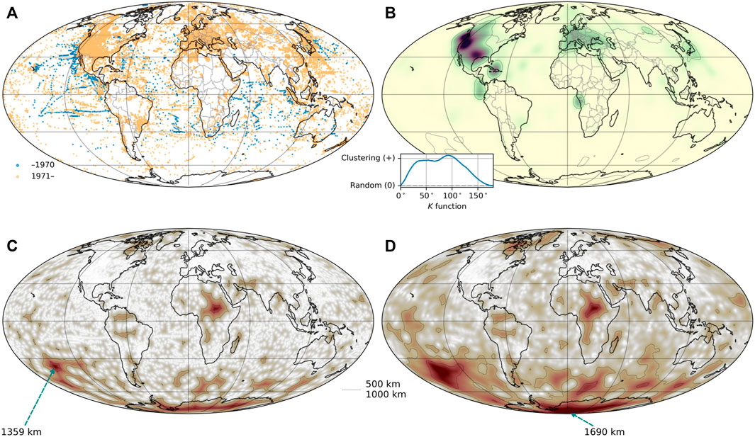
FIGURE 1. Geographic distribution of heat flow measurements. (A) Measurements in IHFC, color coded by year of measurement. (B) Kernel density estimation (KDE) for density of heat flow measurements, using great circle distances and a Gaussian kernel with σ = 400 km. A dotted contour marks the 5% percentile. Inset shows the centred Ripley’s K function plot, where the positive values indicate that measurements are heavily clustered on all scales, with a peak at 90°. (C) Distance to the nearest measurement. The longest distance is 1359 km, at 37°S 148°W in the South Pacific Ocean. (D) Mean distance to nearest ten measurements. The longest distance is 1690 km, at 85°S 8°E in East Antarctica. Contours indicate 500 and 1000 km distances in (C) and (D). Maps are displayed with perceptually linear colour representation (Crameri and Shephard, 2019; Morse et al., 2019) using matplotlib (Hunter, 2007).

One aspect of empirical heat flow studies that has attracted less debate, but has the potential to impact the results, is the representation of the reference heat flow catalogue. Stål et al. (2021) suggest that a focus on economic exploration, particularly, in the Gondwana continents (e.g. Africa and Australia), could lead to sampling bias. Another potential factor that might skew the representation of the catalogue is a tendency to drill in flat and accessible locations within mountainous regions. Heat flow values are sometimes corrected for topographic factors, but not always, and it can be difficult to determine if such corrections have been applied in older studies. Such clarifications are within the scope of the ongoing Global Heat Flow Data Assessment Project of the IHFC catalogue (Fuchs et al., 2021a).

Heat flow measurements have been collected in cumulatively growing databases (e.g. Chapman and Pollack, 1975; Pollack et al., 1993; Hasterok, 2019; Lucazeau, 2019). From analyses of those catalogues, the total heat balance and average heat flow, of Earth have been calculated. The spatial bias has been recognised and causal relationships are used to integrate heat flow from lithospheric age in the oceans (e.g. Lucazeau, 2019) or geological setting (e.g. Davies and Davies, 2010).

In this contribution, we analyse the most recent and extensive heat flow catalogue (Fuchs et al., 2021b) for factors that might bias the distribution and hence impact the integrated heat flow maps. We also discuss qualitative reasons for the uneven distribution and suggest statistical weights of individual samples for use when the catalogue finds ongoing use.

2 Materials and methods

Spatial characteristics of the data are analysed to quantify clustering and misrepresentation. The analysis is carried out using Python libraries: geopandas (Jordahl, 2014), rasterio (Gillies, 2019), and numpy (Harris et al., 2020). Methods are implemented from agrid (Stål and Reading, 2020), a python-based grid for representing multidimensional geophysical data. All code is made available to ensure reproducibility, and all datasets used are provided in open repositories.

2.1 Heat flow database

We include the entire IHFC catalogue (cf. Fuchs et al. 2021b), except for 12 records where positional data is missing. All remaining 74 536 entries are analysed as they appear. We treat every given location as correct and precise; however, this is often not the case for older records.

2.2 Spatial descriptive statistics

We use a kernel density estimate (KDE) function to first appraise the spatial distribution of the heat flow measurements (Figure 1B). The KDE is calculated from a Gaussian kernel (σ = 400 km) applied to the spatial distribution of heat flow measurements. We also calculate the distance in kilometres to the nearest measurement and the mean distance to the nearest ten measurements on a 0.5 ° × 0.5 ° grid (Figures 1C,D). All distance calculations are done using the haversine formula, assuming a spherical Earth.

For an appraisal of clustering, we calculate Ripley’s centred K functions (Dixon, 2014) (Figure 1B). The standard application is modified for great circle distances (Stål, 2022). The distribution of pair-wise distances is also presented as a histogram in Supplementary Figure S2.

2.3 Area weighting

We compute a geometric area weighting, assigning a higher weight to sparse records, and a lower weight to densely located measurements. This approach does not take the geological setting into account. For each record, we first weigh other records by proximity from a Gaussian kernel so that the impact decreases with the distance. We apply three different Gaussian kernels with σ = 50 km, 200 km, and 1000 km. The weight for each record in IHFC is calculated from the inverse proximity weight divided by the mean inverse proximity weight for all records (Supplementary Figure S5).

2.4 Auxiliary variables from categorical maps

We examine the sampling bias in heat flow measurements for eight categorical auxiliary variables. Some do not directly correlate with observed geothermal heat flow but can be used to investigate the spatial distribution. The selection of those variables is based on three criteria:

1) Has global or near-global extent with consistent quality and uniform resolution; however, datasets excluding oceanic settings are considered. Particularly, the observables should be comparable for Gondwanan continents and the rest of the world.

2) Represents parameters with expected auxiliary impact on the heat flow distribution.

3) Is available with open access to a computer-readable format.

Auxiliary variable values at each heat flow location are sampled using spatial join for vector polygon datasets or point sampling to the nearest pixel for data sets provided as rasters. Those values are added as attribute data to the database file analysed (this modified database is provided with supplementary material). The relative reference area distribution of each class is calculated from the dataset used, excluding undefined area. Vector polygon areas are calculated in an equal-area projection, and global rasters are compensated with a function that weights each pixel to the area it represents on a sphere. All tectonic, geological or geomorphometric classes for each auxiliary variable are listed in Figure 2. We also calculate the relative distribution of two cultural datasets to investigate the reasons for the sampling bias (Figure 3).

FIGURE 2

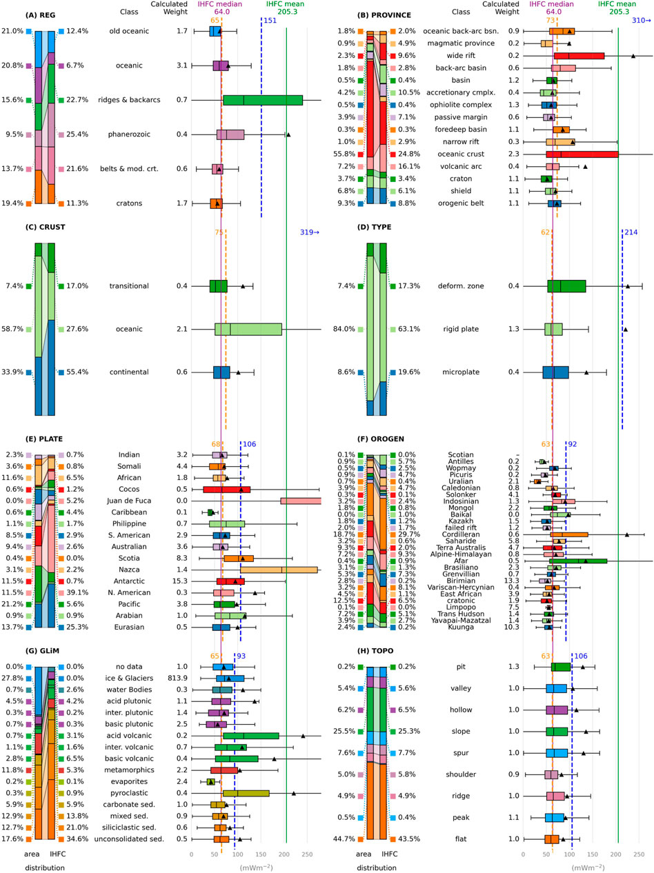
FIGURE 2. (Previous page.) Categorical classes in auxiliary variables, as sampled and heat distribution for each class. (A) Regionalisation from seismic surface wave tomography (Schaeffer and Lebedev, 2015) (B) Province type (Hasterok et al., 2022) (C) Crustal type (Hasterok et al., 2022) (D) Tectonic plate type (Hasterok et al., 2022) (E) Tectonic plate name (Hasterok et al., 2022) (F) Last orogeny (Hasterok et al., 2022) (G) Lithological class (Hartmann and Moosdorf, 2012) (H) Geomorphometric shape (Amatulli et al., 2020) From left to right within each subplot: Percentage of the relative distribution of the class of auxiliary variable calculated for an equal-area projection, shown numerically and as a bar plot (left bar). Percentage of the relative distribution of the class of the location measurement in IHFC are shown as a bar plot (right bar) and numerically. The calculated weight for each class to compensate for the difference between the distributions. The horizontal box plots show the heat flow distribution for measurements within each class. The mean heat flow for each class is indicated by a black triangular marker (▴). The median heat flow for each class is indicated with the vertical line (|) within each box. Note that a few whiskers and bars are cropped (e.g. Juan de Fuca Plate in Figure 2E). Outliers are not indicated. The median and mean values for each class, and the corresponding weighted medians and means, are listed in Supplementary Table S1. Weighted average heat flow for each auxiliary variable shown as a dashed blue vertical line and given numerically in blue at the top. The value is calculated by assigning the mean heat flow for each class to the reference area. The median values for the weighted means are shown as a dashed orange vertical line and a numerical value in orange at the top. The vertical lines indicate the mean (green; 205.3 mWm⁻³) and median (purple; 64 mWm⁻³) values of all IHFC database records (Fuchs et al., 2021b). Abbreviation used in the labels; bsn. = basin, cmplx = complex, interm. = intermediate, belts & mod. crt. = Precambrian belts and modified cratons, sed. = sediments or sedimentary rocks. All heat flow values are given in mW m⁻²; units are omitted to minimise clutter.

FIGURE 3

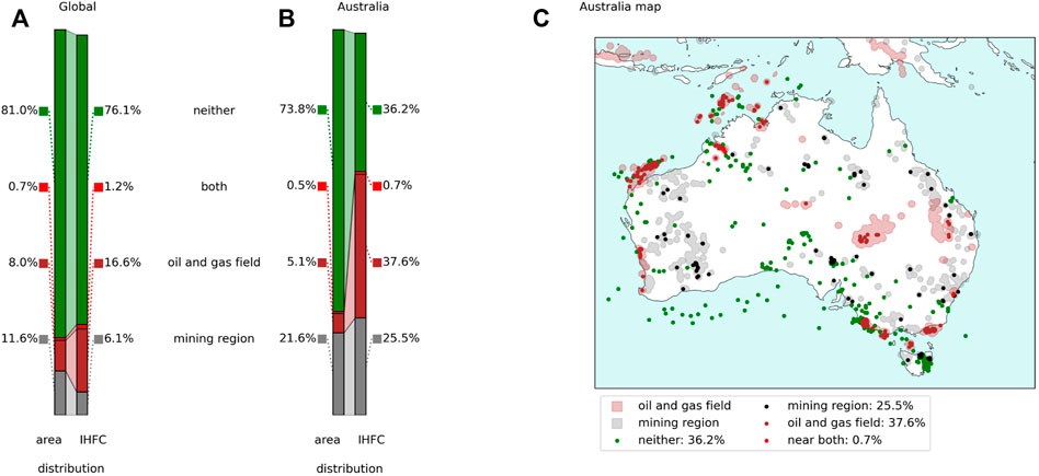
FIGURE 3. Correlation with mining and hydrocarbon prospecting and exploration. (A) The area distribution for mining polygons (grey), oil and gas fields (brown), overlapping mining region and oil field (red), and neither mining nor oil and gas fields near the measurement (green, as explained in Figure 2). The reference land area is the global landmass; however, offshore oil and gas fields are included, making the total slightly over 100%. (B) The Australian area distribution for oil fields (392.591 km²) (Rose et al., 2018) and mining regions (Maus et al., 2020) with a buffer, as described in the text (1.657.683 km²). The reference area is the Australian landmass (7.692.024 km²). (C) Map of Australia showing mine sites (Maus et al., 2020) with a buffer of 0.5° and gas fields (Rose et al., 2018).

2.4.1 Tectonic variables

We include the regionalisation from clustering of surface wave tomography (Schaeffer and Lebedev, 2015) (labelled as REG), which provides a quantitative, robust global regionalisation (Figure 2A). We also include the recent tectonic and geologic province maps (Hasterok et al., 2022), these maps are constructed from refined qualitative and quantitative analyses of published global and regional maps, and auxiliary geoscientific data sets such as earthquake locations and geochronology. We analyse for the following: Province type (PROVINCE), for example, craton, passive margin, basin (Figure 2B); Crust type (CRUST), i.e. continental, oceanic, transitional crust (Figure 2C); Plate type (TYPE), i.e. microplate, rigid plate, deformation zone (Figure 2D). Tectonic plate (PLATE), for example, Philippine Plate, Antarctic Plate, and Somali Plate (Figure 2E). We also investigate the most recent orogeny (OROGEN), for example, Alpine-Himalayan, Grenvillian, and Afar (Figure 2F). This dataset provides a first-order approximation of crustal stabilisation age.

2.4.2 Geological variables

Lithological affiliation is sampled from the GLiM map (Hartmann and Moosdorf, 2012). The map is assembled from existing regional geological maps translated into 16 classes (for example, unconsolidated sediments, metamorphics, and basic volcanic rocks). The relative abundance of each class only considers the land area as the geology of oceanic regions is not provided; however, we include classes such as water bodies, and ice and glaciers (Figure 2G).

2.4.3 Geomorphometric variables

Topographic refraction is a well-known parameter to locally focus heat (Lees et al., 1910). A recent set of geomorphometrics rasters (Amatulli et al., 2020) provides insights into the shape of the topography from a high-resolution global digital elevation model (Yamazaki et al., 2017). One raster with particular relevance for a first appraisal is the geomorphological forms (Jasiewicz and Stepinski, 2013; Amatulli et al., 2018). The shape is associated with ten classes such as ridge, summit, and slope (TOPO, Figure 2H). For efficient area distribution calculation, we sub-sample the raster at a ratio of 1:40 (Supplementary Figure S1). Point sampling at heat flow measurements is done in full resolution, 250 m at the equator, corresponding to 0.00208°.

2.4.4 Cultural variables

We investigate the economic setting for where heat flow measurements have been conducted. Prospecting and exploration are linked to geology as well as infrastructure and accessibility. We count the fraction of heat flow measurements within oil and gas fields (Rose et al., 2018). We also count the number of measurements within 0.5° distance from mining sites, derived from reported activities and infrastructure identified from satellite images (Maus et al., 2020). Cultural auxiliary variable polygons are dissolved to remove any overlapping polygons.

As a reference for both cultural datasets, we use the total area of the Earth’s landmass 148 940 000 km²; however, data points in offshore oil and gas fields are included, and hence the total reference area is slightly larger than 100%. (Figures 3A,B). We also investigate the Australian case for an appraisal of the impact in a region known for mining and hydrocarbon exploration and relevant for an understanding of East Antarctic geothermal heat distribution. The reference Australian landmass area is 7 692 024 km² (Figures 3B,C).

2.5 Calculation of weights

For each auxiliary variable, a weight is calculated for sample balancing as the quotient ratio of the fraction of reference area covered by a given class, and the fraction of heat flow measurements taken from the matching setting:

$w\left(c\right)=\frac{f_A\left(c\right)}{f_N\left(c\right)},(1)$

where w(c) is the calculated weight for each class or category (c), f_A(c) is the area fraction of the reference area; entire globe, terrestrial landmass (TOPO and GliM), or all orogens (OROGEN), and f_N(c) is the fraction of measurements in IHFC located within the area of the class. The weights for each auxiliary variable are assigned to each record for the class it is located within. Weights for four auxiliary variables are shown in Figures 4A–D, and for all variables in Supplementary Figure S3.

FIGURE 4

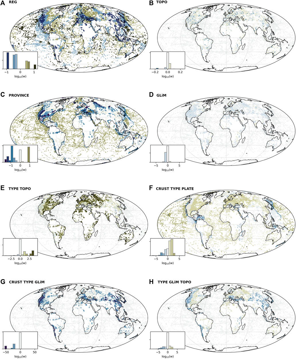
FIGURE 4. Calculated weights for selected categorical variables and suggestions for combined weights. (A) REG (Schaeffer and Lebedev, 2015) (B) Geomorphological forms (Amatulli et al., 2020) (C) Province (Hasterok et al., 2022) (D) GLiM (Hartmann and Moosdorf, 2012) (E) IPF calculated joint weighting from TYPE and TOPO, (F) IPF calculated joint weighting from CRUST, TYPE, and PLATE, (G) IPF calculated joint weighting from TYPE and GLiM, (H) IPF calculated joint weighting from TYPE, GLiM, and TOPO. The weights are displayed as a logarithmic colour representation to allow for the ranges to be compared. Measurements with no weighting (i.e. weight of 1) are shown in grey, those that are weighted down are in blue, and measurements weighted up are shown in brown. The inset histogram shows the relative log–value distribution. Note that the scale differs for each subplot for clarity.

Some auxiliary variables are correlated because they represent comparable properties in their respective studies or by the nature of geological processes (Supplementary Figure S5). Combining weights is not straightforward, and various techniques with different benefits and shortcomings produce diverging results (Reviewed by Kalton and Flores-Cervantes, 2003). A well-established approach is iterative proportional fitting (IPF), sometimes referred to as raking. IPF is an iteratively-calculated weight for each combination of classes between the N variables that satisfies the marginal distribution for each variable. We compute combined weights using the Python package ipfn (Forthommme, 2021). There is no theoretical upper limit to how many variables can be fitted; however, attempts to fit more than four variables return non-robust high weights, and the computational cost increases exponentially with the number of variables. Individual records can be assigned very high weight if underrepresented in more than one auxiliary variable.

We calculate joint weighting for all combinations of 2, 3 or 4 auxiliary variables, yielding a total of ${\sum }_{k=\mathrm{2,3,4}}\left(\genfrac{}{}{0ex}{}{8}{k}\right)=154$ combinations. All fitted weights are added to the catalogue. Weighted mean, weighted median and difference from estimated global average is listed in Supplementary Table S2, S3 and S4.

We assume that a reasonable indication of the soundness of a weighting is that the weighted average is closer to the estimated global average 80 mW m⁻² (Lucazeau, 2019) than the mean of the catalogue, 205 mW m⁻². As such, we rank the weightings by difference from 80 mW m⁻². This is not a universal validation but allows us to consider what properties are meaningful.

3 Results

The map in Figure 1A shows the records in the IHFC. The spatial distribution is also shown as a kernel density estimation in Figure 1B. This smoothed distribution highlights that the highest density of measurements is in the Western United States and Southern Europe. The inset to the bottom-left of Figure 1B shows centered Ripley’s K function. For context, the expected value of the K function for spatially uniform sampling is $\widehat{K}(t)=0$. The measured K function is positive on all scales, indicating clustering.

Figure 1C shows the distance to the nearest IHFC heat flow record, measured from grid cell centres. Central Africa, the Amazon Basin, and parts of the Middle East, have extensive areas with a distance of over 500 km to the nearest record. In parts of interior Africa there are areas with over 1000 km, and up to 1359 km in South Pacific. Figure 1D shows the mean distance to the closest ten measurements. The overall distribution is similar; however notably, the Southern Ocean is highlighted as having only a few measurements representing large areas. For both metrics, Antarctica is exceptionally sparsely surveyed.

In Figure 2, we show the reference and sampled distributions, and the heat flow associated with each class for the eight categorical auxiliary variables. The calculated weights are listed. The horizontal bar charts show the heat distribution within each class. Generally, the mean heat flow values tend to be much higher than the median due to extremely high measurements in active geothermal settings. The difference between the median and mean values of IHFC and the weighted average heat flow indicates the magnitude of the impact on heat flow models from sampling bias. We also calculate the robust mean, excluding 1 and 10% upper and lower percentiles (Supplementary material Table S1).

To better understand the origin of the sampling bias, we extract the economic setting for the measurements: 17.8% of the measurements in IHFC are within the polygons defined as oil and gas fields (Rose et al., 2018), in relation to only 8.7% of the landmass. Meanwhile, 7.3% of the measurements are within 0.5° from a mine, as mapped (Maus et al., 2020), in relation to 12.3% of the global landmass, excluding oceans. Prospective regions are only slightly over-represented on a global average; however strongly pronounced in sparsely populated Australia, where 26.2% of the measurements in IHFC are located in mining areas (c.f. 22.1% by landmass), as defined above, and 38.3% of the measurements are within oil and gas fields (c.f. 5.6% by landmass, Rose et al. 2018). Moreover, many of the remaining measurements are in regions targeted for geothermal heat extraction, e.g. North West Tasmania and South-Western Victoria (Holgate et al., 2010; Bahadori et al., 2013). Figure 3C shows the Australian records in IHFC and the polygons used to define mining and oil and gas fields.

Figure 4 shows the weights calculated. Figure 4A shows the weights derived from seismic tomography regionalisation (Schaeffer and Lebedev, 2015), highlighting the general under-representation of the oceanic crust. Figure 4B shows the smaller weights from geomorphometrics (Amatulli et al., 2020). For this analysis, local rather than global and reg ional distribution impacts the weight. Figure 4C shows the weights based on the province (Hasterok et al., 2022). Figure 4D shows the weights from lithologies (Hartmann and Moosdorf, 2012). Oceans are set to a weight of 1. All ten maps are provided in Supplementary material Figure S4.

We now consider selected weights derived for the classes in each auxiliary variable using IPF, as described in Section 2.5.

The IPF calculated weighting from TYPE and TOPO produce a weighted average of 84 mW m⁻², this is closest to the global mean (Pollack et al., 1993; Lucazeau, 2019), and also the lowest weighted mean for any fitted weighting. The weighted median is 58 mW m⁻², which is lower than the median of IHFC, 64 mW m⁻² (Figure 4E). IPF calculated weighting from the three variables CRUST, TYPE, and PLATE yield a weighted mean of 93 mW m⁻², which is also close to expected global average. The weighted median is 60 mW m⁻² (Figure 4F). An IPF calculated weighting from a combination with the potential to capture both tectonic and geological misrepresentation, TYPE and GLiM, gives a weighted mean of 95 mW m⁻², and a weighted median is 58 mW m⁻² (Figure 4G). An IPF calculated weighting from TYPE, GLiM and TOPO represents tectonic, geological and topographic settings. The weighted mean for this combination is 145 mW m⁻², and the weighted median is 59 mW m⁻² (Figure 4H).

From all variables considered, some extreme weights are suggested. In order to compensate for the sparse measurements from GLiM class glaciers and ice sheets, measurements for those two classes are calculated to have a weight of 813.9 (Figure 2). Other underrepresented tectono-geographical regions include, as a most recent orogen, the Birimian Orogen, Kuunga Orogen and particularly the Scotian Orogen, where no heat flow measurements are catalogued. Generally, Gondwana and the oceanic crust are underrepresented.

4 Discussion

We have shown that the distribution of heat flow measurements is spatially biased and does not fully represent the Earth’s geometric, tectonic, geological or geomorphometric disposition. This conclusion is readily seen from the clustering of measurements (Figure 1B), and in the context of eight auxiliary variables, whereby we found that some settings are overrepresented whilst others are correspondingly underrepresented. The selection of those variables is somewhat arbitrary; however, together, they represent a meaningful range of parameters that should be expected to impact the distribution of geothermal heat. The scope of this contribution is not to analyse the relation between observables and geothermal heat, as has been done in previous studies (e.g. Davies and Davies, 2010; Goutorbe et al., 2011), but to investigate how well the heat flow catalogue represents the Earth’s surface.

The calculated weights from each variable compensate for the bias, and the combined fitted weights provide individually optimised weights for each record in IHFC. The somewhat diverging results highlight the need for caution when weighting is applied in empirical models. The choice of weights depends on the scale of the model and relevance of the variables used. It would be tempting to evaluate the weights based on their performance to reduce prediction misfits in existing empiric models; however, such an appraisal will necessarily contain the same bias. A useful test case could be cross-validation of a sufficiently large subset of the heat flow catalogue that can be shown to truly represent a random sampling of the Earth, and of good quality. Unfortunately, given that some settings are strongly underrepresented, such a sample distribution is not yet possible. With empirically driven heat flow models, there is potential to further explore how the weighting and processing of reference measurements can impact the results. Some observables, such as the distance to volcanoes, have been shown to have large impact (Lösing and Ebbing, 2021); however, the sensitivity changes if weights are applied, and in many cases extreme geothermal settings are weighted down.

One potential shortcoming in this study is that we have assumed that the coordinates of the measurements are given correctly and accurately to match the auxiliary variables; this is often not the case. The surprisingly low bias in the geomorphometrics variable might be, at least partially, explained by imprecise positions that sample random geomorphological forms in the vicinity rather than the actual topographic shape right at the borehole.

From an assumption that weighted mean and median values from the catalogue should approach the qualitative estimates of the global heat flow distribution, the closest weighted mean is given precedence in our interpretation. The total Earth heat loss is estimated to be 40–42 TW, or 80 mW m⁻² (Lucazeau, 2019). Earlier studies come to similar results (e.g. Pollack et al., 1993). Most weighted mean values are closer to this average, suggesting that weight applied to metrics of the catalogue can improve the prediction if applied carefully.

Weights derived from one auxiliary variable, that generate weighted averages close to the expected global value: Last orogeny (OROGEN) average is +12 mW m⁻² compared to global average, shallow geology (GLiM), +13 mW m⁻², geomorphometric shapes (TOPO), +26 mW m⁻², and tectonic plate, +26 mWm⁻². The fitted weight from plate type (TYPE) and topography (TOPO) (Figure 4E) produces a close value of +4 mWm⁻², however we have concerns regarding the validity of the geomorphometrics (TOPO), as the coordinates given in the catalogue might not be precise enough. Moreover, marine data is note weighted to topography. Plate type (TYPE) and shallow geology (GLiM) also generate a weighting that is similar to the global average at +16 mWm⁻² (Figure 4G). A qualitative reasoning of what processes would impact heat flow on different scales, is represented by weighting for tectonic setting (TYPE), shallow geology (GLiM) and topography (TOPO). This combination gives a weighted mean difference of +65 mWm⁻² (Figure 4H).

The spatial sampling bias is consistent with the challenges and lack of incentives to conduct investigations in remote regions or developing countries. More measurements of the thermal gradient have likely been conducted for prospecting and exploration reasons in some of such sparse areas; however, the results are not included in heat flow compilations and the understanding of some areas suffers from very sparse records (Figures 1C,D, (Discussed by e.g. Brigaud et al., 1985; Lesquer and Vasseur 1992; Noorollahi et al., 2009; Yousefi et al., 2010)). We also suggest that the quality of the measurements varies spatially. Some assumptions might be outdated in areas where older measurements dominate (Figure 1A). If one were to use borehole data alone, the marine portions of the map would be even more sparsely sampled, except near oil and gas provinces.

Acknowledging the achievement of the cumulative heat flow catalogues, the scope of this contribution is to support and add value to the ongoing, substantial undertaking to coordinate a representative compilation of measurements.

We make six recommendations from the results of this study:

1) Empirical heat flow model developers should consider applying weights when using the reference database and investigate how this can reduce uncertainty and misfit.

2) The spatial coordinates of heat flow measurements should, whenever possible, be amended such that they are sufficiently precise and accurate to facilitate statistical analysis of refraction from topography and shallow geology. This is viable thanks to the availability of global high resolution digital elevation model and refined geological maps.

3) Attribute data could be added to heat flow records, including information about geological setting and uncertainties, to assist in future appraisals. Particularly, the lithospheric age of the site should be included for marine heat flow values.

4) In the ongoing assessment project of the IHFC database, highly weighted existing records should be assessed first, as they represent underrepresented settings.

5) All heat flow measurements are valuable additions; however, underrepresented regions and settings should be prioritised when new data is incorporated into IHFC.

6) To truly improve the global thermal representation of the catalogue, underrepresented regions and settings should be prioritised for future new heat flow measurements, particularly within the Gondwanan continents Antarctica, Africa, and Australia, Southern Ocean and South Pacific Ocean; and particularly in regions without an immediate interest for mineral or hydrocarbon exploration.

Data availability statement

Publicly available datasets were analyzed in this study. This data can be found here: https://ihfc-iugg.org/products/global-heat-flow-database/data https://zenodo.org/record/6586972 https://doi.org/10.1594/PANGAEA.910894 https://edx.netl.doe.gov/dataset/global-oil-gas-features-database https://github.com/TobbeTripitaka/heat-flow-sampling-bias.

Author contributions

TS conceived the presented idea, developed the theory and performed the computations. AR and RT verified and advised on the analytical methods. AR, SF, JH, and ML supervised the findings of this work. All authors discussed the results and contributed to the final manuscript.

Funding

This research was supported by the Australian Research Council through ARC DP190100418, ARC Special Research Initiative, Australian Centre for Excellence in Antarctic Science (Project Number SR200100008), and ARC DP180104074. Additional support was provided through the Deutsche Forschungsgemeinschaft (DFG) in the framework of the priority programme “Antarctic Research with comparative investigations in Arctic ice areas” (Grant No. EB 255/8-1).

Acknowledgments

We thank Matthew Cracknell and Nick Direen for their insights into ore prospecting and spatial datasets of mining sites. We also thank the two reviewers for their thoughtful inputs to our manuscript. Discussions informing this review were facilitated by the Scientific Committee on Antarctic Research, Instabilities and Thresholds in Antarctica, sub-committee on Geothermal Heat Flow (SCAR, INSTANT).

Conflict of interest

The authors declare that the research was conducted in the absence of any commercial or financial relationships that could be construed as a potential conflict of interest.

Publisher’s note

All claims expressed in this article are solely those of the authors and do not necessarily represent those of their affiliated organizations, or those of the publisher, the editors and the reviewers. Any product that may be evaluated in this article, or claim that may be made by its manufacturer, is not guaranteed or endorsed by the publisher.

Supplementary material

The Supplementary Material for this article can be found online at: https://www.frontiersin.org/articles/10.3389/feart.2022.963525/full#supplementary-material

References

Amatulli, G., Domisch, S., Tuanmu, M. N., Parmentier, B., Ranipeta, A., Malczyk, J., et al. (2018). Data descriptor: A suite of global, cross-scale topographic variables for environmental and biodiversity modeling. Sci. Data 5, 180040. doi:10.1038/sdata.2018.40

PubMed Abstract | CrossRef Full Text | Google Scholar

Amatulli, G., McInerney, D., Sethi, T., Strobl, P., and Domisch, S. (2020). Geomorpho90m, empirical evaluation and accuracy assessment of global high-resolution geomorphometric layers. Sci. Data 7, 162. doi:10.1038/s41597-020-0479-6

PubMed Abstract | CrossRef Full Text | Google Scholar

An, M., Wiens, D. A., Zhao, Y., Feng, M., Nyblade, A., Kanao, M., et al. (2015). Temperature, lithosphere-asthenosphere boundary, and heat flux beneath the Antarctic Plate inferred from seismic velocities. J. Geophys. Res. Solid Earth 120, 8720–8742. doi:10.1002/2015JB011917

CrossRef Full Text | Google Scholar

Artemieva, I. M. (2022). Antarctica ice sheet basal melting enhanced by high mantle heat. Earth-Science Rev. 226, 103954. doi:10.1016/j.earscirev.2022.103954

CrossRef Full Text | Google Scholar

Artemieva, I. (2011). The Lithosphere: An interdisciplinary approach. Cambridge: Press, Cambridge University.

Google Scholar

Bahadori, A., Zendehboudi, S., and Zahedi, G. (2013). Retracted: A review of geothermal energy resources in Australia: Current status and prospects. Renew. Sustain. Energy Rev. 21, 29–34. doi:10.1016/j.rser.2012.12.020

CrossRef Full Text | Google Scholar

Beardsmore, G. R., and Cull, J. P. (2001). Crustal heat flow. Cambridge: Press, Cambridge University. doi:10.1017/cbo9780511606021

CrossRef Full Text | Google Scholar

Brigaud, F., Lucazeau, F., Ly, S., and Sauvage, J. F. (1985). Heat flow from the west african shield. Geophys. Res. Lett. 12, 549–552. doi:10.1029/gl012i009p00549

CrossRef Full Text | Google Scholar

Burton-Johnson, A., Dziadek, R., and Martin, C. (2020). Geothermal heat flow in Antarctica: Current and future directions. Cryosphere Discuss. 14, 1–45. doi:10.5194/tc-2020-59

CrossRef Full Text | Google Scholar

Burton-Johnson, A., Halpin, J. A., Whittaker, J. M., Graham, F. S., and Watson, S. J. (2017). A new heat flux model for the Antarctic Peninsula incorporating spatially variable upper crustal radiogenic heat production. Geophys. Res. Lett. 44, 5436–5446. doi:10.1002/2017GL073596

CrossRef Full Text | Google Scholar

Chapman, D. S., and Pollack, H. N. (1975). Global heat flow: A new look. Earth Planet. Sci. Lett. 28, 23–32. doi:10.1016/0012-821X(75)90069-2

CrossRef Full Text | Google Scholar

Colgan, W., Wansing, A., Mankoff, K., Lösing, M., Hopper, J., Louden, K., et al. (2022). Greenland geothermal heat flow database and map (version 1). Earth Syst. Sci. Data 14, 2209–2238. doi:10.5194/essd-14-2209-2022

CrossRef Full Text | Google Scholar

[Dataset] Crameri, F., and Shephard, G. E. (2019). Scientific colour maps. doi:10.5281/zenodo.3596401

CrossRef Full Text | Google Scholar

Cull, J. P., Houseman, G. A., Muir, P. M., and Paterson, H. L. (1988). Geothermal signatures and uranium ore deposits on the stuart shelf of South Australia. Explor. Geophys. 19, 34–38. doi:10.1071/EG988034

CrossRef Full Text | Google Scholar

Davies, J. H., and Davies, D. R. (2010). Earth’s surface heat flux. Solid earth. 1, 5–24. doi:10.5194/se-1-5-2010

CrossRef Full Text | Google Scholar

Davies, J. H. (2013). Global map of solid Earth surface heat flow. Geochem. Geophys. Geosyst. 14, 4608–4622. doi:10.1002/ggge.20271

CrossRef Full Text | Google Scholar

Dickson, M. H., and Fanelli, M. (2013). Geothermal energy: Utilization and technology. Oxfordshire, England, UK: Routledge.

Google Scholar

Dixon, P. M. (2014). Ripley’s K function. Wiley StatsRef Stat. Ref. Online 3, 1796–1803. doi:10.1002/9781118445112.stat07751

CrossRef Full Text | Google Scholar

Dziadek, R., Gohl, K., Diehl, A., and Kaul, N. (2017). Geothermal heat flux in the Amundsen Sea sector of West Antarctica: New insights from temperature measurements, depth to the bottom of the magnetic source estimation, and thermal modeling. Geochem. Geophys. Geosyst. 18, 2657–2672. doi:10.1002/2016GC006755

CrossRef Full Text | Google Scholar

Ebbing, J., Gernigon, L., Pascal, C., Olesen, O., and Osmundsen, P. T. (2009). A discussion of structural and thermal control of magnetic anomalies on the mid-Norwegian margin. Geophys. Prospect. 57, 665–681. doi:10.1111/j.1365-2478.2009.00800.x

CrossRef Full Text | Google Scholar

[Dataset] Forthommme, D. (2021). Iterative proportional fitting for Python with N dimensions.

Google Scholar

Fuchs, S., Beardsmore, G., Chiozzi, P., Espinoza-Ojeda, O. M., Gola, G., Gosnold, W., et al. (2021a). A new database structure for the IHFC global heat flow database. ijthfa. 4, 1–14. doi:10.31214/ijthfa.v4i1.62

CrossRef Full Text | Google Scholar

Fuchs, S., Norden, B., and Commission, I. H. F. (2021b). The global heat flow database: Release 2021. Potsdam: GFZ Data Services, 1–73. doi:10.5880/fidgeo.2021.014

CrossRef Full Text | Google Scholar

Fukahata, Y., and Matsu’ura, M. (2001). Correlation between surface heat flow and elevation and its geophysical implication. Geophys. Res. Lett. 28, 2703–2706. doi:10.1029/2000GL012653

CrossRef Full Text | Google Scholar

Gard, M., and Hasterok, D. (2021). A global Curie depth model utilising the equivalent source magnetic dipole method. Phys. Earth Planet. Interiors 313, 106672. doi:10.1016/j.pepi.2021.106672

CrossRef Full Text | Google Scholar

Gerard, R., Langseth, M. G., and Ewing, M. (1962). Thermal gradient measurements in the water and bottom sediment of the Western Atlantic. J. Geophys. Res. 67, 785–803. doi:10.1029/JZ067i002p00785

CrossRef Full Text | Google Scholar

Gillies, S. (2019). Rasterio Documentation.

Google Scholar

Goes, S., Hasterok, D., Schutt, D. L., and Klöcking, M. (2020). Continental lithospheric temperatures: A review. Phys. Earth Planet. Interiors 306, 106509. doi:10.1016/j.pepi.2020.106509

CrossRef Full Text | Google Scholar

Goutorbe, B., Poort, J., Lucazeau, F., and Raillard, S. (2011). Global heat flow trends resolved from multiple geological and geophysical proxies. Geophys. J. Int. 187, 1405–1419. doi:10.1111/j.1365-246X.2011.05228.x

CrossRef Full Text | Google Scholar

Greve, R., and Hutter, K. (1995). Polythermal three-dimensional modelling of the Greenland ice sheet with varied geothermal heat flux. Ann. Glaciol. 21, 8–12. doi:10.3189/S0260305500015524

CrossRef Full Text | Google Scholar

Haeger, C., Kaban, M. K., Tesauro, M., Petrunin, A. G., and Mooney, W. D. (2019). 3-D density, thermal, and compositional model of the antarctic lithosphere and implications for its evolution. Geochem. Geophys. Geosyst. 20, 688–707. doi:10.1029/2018GC008033

CrossRef Full Text | Google Scholar

Harris, C. R., Millman, K. J., van der Walt, S. J., Gommers, R., Virtanen, P., Cournapeau, D., et al. (2020). Array programming with NumPy. Nature 585, 357–362. doi:10.1038/s41586-020-2649-2

PubMed Abstract | CrossRef Full Text | Google Scholar

Hartmann, J., and Moosdorf, N. (2012). The new global lithological map database GLiM: A representation of rock properties at the earth surface. Geochem. Geophys. Geosyst. 13, 1–37. doi:10.1029/2012GC004370

CrossRef Full Text | Google Scholar

Hasterok, D. (2013). A heat flow based cooling model for tectonic plates. Earth Planet. Sci. Lett. 361, 34–43. doi:10.1016/j.epsl.2012.10.036

CrossRef Full Text | Google Scholar

Hasterok, D., and Gard, M. (2016). Utilizing thermal isostasy to estimate sub-lithospheric heat flow and anomalous crustal radioactivity. Earth Planet. Sci. Lett. 450, 197–207. doi:10.1016/j.epsl.2016.06.037

CrossRef Full Text | Google Scholar

Hasterok, D., Gard, M., and Webb, J. (2018). On the radiogenic heat production of metamorphic, igneous, and sedimentary rocks. Geosci. Front. 9, 1777–1794. doi:10.1016/j.gsf.2017.10.012

CrossRef Full Text | Google Scholar

Hasterok, D., Halpin, J., Collins, A., Hand, M., Kreemer, C., Gard, M., et al. (2022). New maps of global geological provinces and tectonic plates. Earth-Science Rev. 231, 104069. doi:10.1016/j.earscirev.2022.104069

CrossRef Full Text | Google Scholar

[Dataset] Hasterok, D. (2019). Thermoglobe. Available at: www.heatflow.org.

Google Scholar

Holgate, F. L., Goh, H. K., Wheller, G., and Lewis, R. G. (2010). “The central tasmanian geothermal anomaly: A prospective new egs province in Australia,” in Proceedings World Geothermal Congress, Bali, Indonesia, 1–6.

Google Scholar

Huang, S., Pollack, H. N., and Shen, P. Y. (1997). Late Quaternary temperature changes seen in world-wide continental heat flow measurements. Geophys. Res. Lett. 24, 1947–1950. doi:10.1029/97GL01846

CrossRef Full Text | Google Scholar

Hunter, J. D. (2007). Matplotlib: A 2D graphics environment. Comput. Sci. Eng. 9, 90–95. doi:10.1109/MCSE.2007.55

CrossRef Full Text | Google Scholar

Hyndman, R. D., Davis, E. E., and Wright, J. A. (1979). The measurement of marine geothermal heat flow by a multipenetration probe with digital acoustic telemetry and insitu thermal conductivity. Mar. Geophys. Res. 4, 181–205. doi:10.1007/BF00286404

CrossRef Full Text | Google Scholar

Jasiewicz, J., and Stepinski, T. F. (2013). Geomorphons-a pattern recognition approach to classification and mapping of landforms. Geomorphology 182, 147–156. doi:10.1016/j.geomorph.2012.11.005

CrossRef Full Text | Google Scholar

Jaupart, C., Mareschal, J. C., and Iarotsky, L. (2016). Radiogenic heat production in the continental crust. Lithos 262, 398–427. doi:10.1016/j.lithos.2016.07.017

CrossRef Full Text | Google Scholar

Jordahl, K. (2014). GeoPandas: Python tools for geographic data. Available at: https://github.com/geopandas/geopandas.

Google Scholar

Kalton, G., and Flores-Cervantes, I. (2003). Weighting methods. J. Official Statistics 19, 81–97.

Google Scholar

Karlsson, N. B., Solgaard, A. M., Mankoff, K. D., Gillet-Chaulet, F., MacGregor, J. A., Box, J. E., et al. (2021). A first constraint on basal melt-water production of the Greenland ice sheet. Nat. Commun. 12, 3461. doi:10.1038/s41467-021-23739-z

PubMed Abstract | CrossRef Full Text | Google Scholar

Kelvin, W. T. (1863). On the secular cooling of the Earth. Trans. R. Soc. Edinb. 23, 157–170.

Google Scholar

Lees, C. H. C. H., Districts, R.-a., and Lees, C. H. C. H. (1910). On the shapes of the isogeotherms under mountain ranges in radio-active districts. Proc. R. Soc. Lond. Ser. A, Contain. Pap. a Math. Phys. Character 83, 339–346. doi:10.1098/rspa.1910.0022

CrossRef Full Text | Google Scholar

Lesquer, A., and Vasseur, G. (1992). Heat-flow constraints on the West African lithosphere structure. Geophys. Res. Lett. 19, 561–564. doi:10.1029/92GL00263

CrossRef Full Text | Google Scholar

Li, M., Huang, S., Dong, M., Xu, Y., Hao, T., Wu, X., et al. (2021). Prediction of marine heat flow based on the random forest method and geological and geophysical features. Mar. Geophys. Res. 42, 30. doi:10.1007/s11001-021-09452-y

CrossRef Full Text | Google Scholar

Lösing, M., and Ebbing, J. (2021). Predicting geothermal heat flow in Antarctica with a machine learning approach. JGR. Solid Earth 126, 1–32. doi:10.1029/2020JB021499

CrossRef Full Text | Google Scholar

Lösing, M., Ebbing, J., and Szwillus, W. (2020). Geothermal heat flux in Antarctica: Assessing models and observations by bayesian inversion. Front. Earth Sci. (Lausanne). 8, 1–13. doi:10.3389/feart.2020.00105

CrossRef Full Text | Google Scholar

Lucazeau, F. (2019). Analysis and mapping of an updated terrestrial heat flow data set. Geochem. Geophys. Geosyst. 20, 4001–4024. doi:10.1029/2019GC008389

CrossRef Full Text | Google Scholar

Mansure, A. J., and Reiter, M. (1979). A vertical groundwater movement correction for heat flow. J. Geophys. Res. 84, 3490–3496. doi:10.1029/JB084iB07p03490

CrossRef Full Text | Google Scholar

Martos, Y. M., Catalán, M., Jordan, T. A., Golynsky, A., Golynsky, D., Eagles, G., et al. (2017). Heat flux distribution of Antarctica unveiled. Geophys. Res. Lett. 44 (11), 426. doi:10.1002/2017GL075609

CrossRef Full Text | Google Scholar

Maus, V., Giljum, S., Gutschlhofer, J., da Silva, D. M., Probst, M., Gass, S. L., et al. (2020). A global-scale data set of mining areas. Sci. Data 7, 289. doi:10.1038/s41597-020-00624-w

PubMed Abstract | CrossRef Full Text | Google Scholar

Morse, P. E., Reading, A. M., and Stål, T. (2019). Well-posed geoscientific visualization through interactive color mapping. Front. Earth Sci. (Lausanne). 7, 0–17. doi:10.3389/feart.2019.00274

CrossRef Full Text | Google Scholar

Noorollahi, Y., Yousefi, H., Itoi, R., and Ehara, S. (2009). Geothermal energy resources and development in Iran. Renew. Sustain. Energy Rev. 13, 1127–1132. doi:10.1016/j.rser.2008.05.004

CrossRef Full Text | Google Scholar

Pasquale, V., Verdoya, M., and Chiozzi, P. (2014). SPRINGER briefs in earth sciences geothermics heat flow in the lithosphere.

Google Scholar

Pattyn, F. (2010). Antarctic subglacial conditions inferred from a hybrid ice sheet/ice stream model. Earth Planet. Sci. Lett. 295, 451–461. doi:10.1016/j.epsl.2010.04.025

CrossRef Full Text | Google Scholar

Podugu, N., Ray, L., Singh, S. P., and Roy, S. (2017). Heat flow, heat production, and crustal temperatures in the Archaean Bundelkhand craton, north-central India: Implications for thermal regime beneath the Indian shield. J. Geophys. Res. Solid Earth 122, 5766–5788. doi:10.1002/2017JB014041

CrossRef Full Text | Google Scholar

Pollack, H. N., and Chapman, D. S. (1977). Mantle heat flow. Earth Planet. Sci. Lett. 34, 174–184. doi:10.1016/0012-821X(77)90002-4

CrossRef Full Text | Google Scholar

Pollack, H. N., Hurter, S. J., and Johnson, J. R. (1993). Heat flow from the Earth’s interior: Analysis of the global data set. Rev. Geophys. 31, 267–280. doi:10.1029/93RG01249

CrossRef Full Text | Google Scholar

Rose, K., Bauer, J., Baker, V., Barkhurst, A., Bean, A., DiGiulio, J., et al. (2018). “Global oil & gas features database,” in Tech. rep. (Pittsburgh, PA, Morgantown, WV ….National energy technology laboratory (NETL).

Google Scholar

Royden, L., and Sclater, J. G. (1980). Continental margin subsidence and heat flow: Important parameters in formation of petroleum hydrocarbons. Am. Assoc. Pet. Geol. Bull. 64. doi:10.1306/2F91894B-16CE-11D7-8645000102C1865D

CrossRef Full Text | Google Scholar

Šafanda, J., Szewczyk, J., and Majorowicz, J. (2004). Geothermal evidence of very low glacial temperatures on a rim of the Fennoscandian ice sheet. Geophys. Res. Lett. 31, 4–7. doi:10.1029/2004GL019547

CrossRef Full Text | Google Scholar

Schaeffer, A. J., and Lebedev, S. (2015). “Global heterogeneity of the lithosphere and underlying mantle: A seismological appraisal based on multimode surface-wave dispersion analysis, shear-velocity tomography, and tectonic regionalization,” in The Earth’s heterogeneous mantle: A geophysical, geodynamical, and geochemical perspective (New York City: Springer International Publishing), 3–46. doi:10.1007/978-3-319-15627-9_1

CrossRef Full Text | Google Scholar

Shalaby, M. R., Hakimi, M. H., and Abdullah, W. H. (2011). Geochemical characteristics and hydrocarbon generation modeling of the jurassic source rocks in the shoushan basin, north Western desert, Egypt. Mar. Petroleum Geol. 28, 1611–1624. doi:10.1016/j.marpetgeo.2011.07.003

CrossRef Full Text | Google Scholar

Shen, W., Wiens, D. A., Lloyd, A. J., and Nyblade, A. A. A. (2020). A geothermal heat flux map of Antarctica empirically constrained by seismic structure. Geophys. Res. Lett. 47, 0–2. doi:10.1029/2020GL086955

CrossRef Full Text | Google Scholar

[Dataset] Stål, T., Reading, A., Fuchs, S., Halpin, J., Lösing, M., and Turner, R. (2022). Understanding sampling bias in the global heat flow compilation. doi:10.5281/zenodo.6830577

CrossRef Full Text | Google Scholar

Stål, T., and Reading, A. M. (2020). A grid for multidimensional and multivariate spatial representation and data processing. J. Open Res. Softw. 8, 2–10. doi:10.5334/jors.287

CrossRef Full Text | Google Scholar

Stål, T., Reading, A. M., Halpin, J. A., Phipps, S. J., Whittaker, J. M., Steven J, P., et al. (2020). The antarctic crust and upper mantle: A flexible 3D model and software framework for interdisciplinary research. Front. Earth Sci. (Lausanne). 8, 1–19. doi:10.3389/feart.2020.577502

CrossRef Full Text | Google Scholar

Stål, T., Reading, A. M., Halpin, J. A., and Whittaker, J. M. (2021). Antarctic geothermal heat flow model: Aq1. Geochem. Geophys. Geosyst. 22, 1–22. doi:10.1029/2020GC009428

CrossRef Full Text | Google Scholar

[Dataset] Stål, T. (2022). Tobbetripitaka/ripley:. doi:10.5281/zenodo.6865006

CrossRef Full Text | Google Scholar

Von Herzen, R. P., and Uyeda, S. (1963). Heat flow through the eastern Pacific ocean floor. J. Geophys. Res. 68, 4219–4250. doi:10.1029/JZ068i014p04219

CrossRef Full Text | Google Scholar

Yamazaki, D., Ikeshima, D., Tawatari, R., Yamaguchi, T., O’Loughlin, F., Neal, J. C., et al. (2017). A high-accuracy map of global terrain elevations. Geophys. Res. Lett. 44, 5844–5853. doi:10.1002/2017GL072874

CrossRef Full Text | Google Scholar

Yousefi, H., Noorollahi, Y., Ehara, S., Itoi, R., Yousefi, A., Fujimitsu, Y., et al. (2010). Developing the geothermal resources map of Iran. Geothermics 39, 140–151. doi:10.1016/j.geothermics.2009.11.001

CrossRef Full Text | Google Scholar