Automatized localization of induced geothermal seismicity using robust time-domain array processing

1 Introduction

Geothermal energy plays an important role in the transition of the energy sector towards sustainable resources. Unfortunately, high-pressure injection of geothermal fluids is often associated with weak to moderate seismicity (e.g., Cornet et al., 1997; Cuenot et al., 2008 or Evans et al., 2012). To minimize the seismic hazard, it is crucial to continuously monitor the injection and production processes and localize associated induced seismicity. A reliable and transparent monitoring also helps to increase the public acceptance of existing and future geothermal projects.

Induced seismicity usually relates to man-made stress perturbations of the subsurface, frequently interfering with the local tectonic stress field, and resulting in earthquake activity (e.g., Grünthal, 2014). It can occur in the context of mining, hydrocarbon or shale gas extraction, wastewater disposal, and geothermal energy production (see, e.g., Suckale, 2010; Grünthal, 2014; Farahbod et al., 2015; Weingarten, et al., 2015). Mechanisms that drive induced seismicity in geothermal environments include pore-pressure and temperature increase, volume change due to fluid withdrawal or injection, and chemical alteration of fracture surfaces (Majer et al., 2007; Zang et al., 2014). Commercial geothermal energy production requires a high geothermal gradient and is therefore often located in active tectonic regions (Brune & Thatcher, 2002). The size and rate of seismicity is then defined by the injection volume (and rate), the orientation of the tectonic stress field relative to the pore pressure increase and the extent of the deviatoric stress field within the local fault system (Cornet & Julien, 1989; Cornet & Jianmin, 1995; Brune & Thatcher, 2002). Grünthal (2014) analyzes the annual frequency-magnitude distribution of induced geothermal seismicity in central Europe in the period from 2000 to 2011 and compares it to the natural earthquake activity in the region. The results show that induced geothermal events with local magnitudes above M_L 2.0 are rare if compared to tectonic earthquakes. However, the intensity of micro-seismicity (M_L < 2.0) is significant, with a b-value of 1.94 (±0.21).

To understand the physical processes during a geothermal stimulation and to establish a reliable seismic hazard assessment, the detection and localization of induced geothermal micro-seismicity has gained more and more relevance (Plenkers et al., 2013). Unfortunately, the preferred locations of geothermal reservoirs lie beneath sedimentary basins, which are often densely populated. This significantly aggravates the detection process due to seismic wave attenuation and an increased level of seismic background noise (Wilson et al., 2002; Plenkers et al., 2013).

Conventional short-/long-term triggers (STA/LTA) will likely fail under complex noise conditions and advanced detection methods are required (Withers et al., 1998). Plenkers et al. (2013) apply a template correlation trigger to detect micro-seismicity related to a stimulation test in the Landau deep-geothermal reservoir. A similar approach is introduced by Vasterling et al. (2017), who use the envelope of recorded seismograms to establish a real-time detector based on template correlation. Joswig (1990) and Sick et al. (2015) use (unsupervised) sonogram pattern recognition for event detection. More recent applications focus on deep-learning approaches, such as convolutional neural networks, to monitor induced (micro-) seismicity and to establish automatized seismic phase picking (e.g., Zhu & Beroza, 2019; Mousavi et al., 2020; Wang et al., 2020; Johnson et al., 2021; Li et al., 2022). Further methods to obtain automatized seismic phase arrivals include autoregressive (AR) prediction (e.g., Takanami & Kitagawa, 1988; Küperkoch et al., 2012), sometimes combined with the Akaike-Information-Criterion (AR-AIC; Akaike, 1973; Leonard & Kennett, 1999; Sleeman & van Eck, 1999), higher-order statistics (e.g., Küpperkoch, 2010) or relative travel-time determination via multi-channel cross correlation (e.g., VanDecar & Crosson, 1990).

In contrast to seismic networks, seismic arrays are located outside the source region and can be used to measure the back azimuth and horizontal apparent velocity of an incoming seismic signal, even without clear phase onsets (Rost & Thomas, 2002). Seismic arrays have been frequently used for earthquake detection on a global, regional, and local scale. This includes studies on the Earth’s (fine-scale) structure, detection of human-induced seismicity, volcano monitoring (cf. Rost & Thomas, 2002 or Schweitzer et al., 2012 and references therein), and ocean-bottom arrays (Krüger et al., 2020). Following its initial purpose of detecting nuclear explosions (e.g., Douglas et al., 1999), different studies utilize seismic arrays for seismic risk assessment. Gibbons et al. (2005), for example, use autoregressive prediction and narrowband f-k analysis for a case study to monitor mining blasts. Li and Zhan (2018) use a distributed acoustic sensing array and template matching to detect induced geothermal seismicity in the Brady field. Further examples include real-time infrasound monitoring at the Alaska Volcano Observatory (Coombs et al., 2018) and the real-time array data processing software RETREAT (Smith & Bean, 2020), developed with a focus on volcano monitoring and volcanic tremor.

Most standard array processing methods apply beamforming in the time- (beam power analysis; see King et al., 1975; 1976) or frequency-wavenumber domain (f-k analysis; see Capon, 1969). Both approaches perform calculations of the beam power over a predefined slowness grid in the horizontal ($x$-$y$) plane and search for its maximum. Further established methods are progressive multi-channel correlation (Cansi, 1995), which evaluates a travel time closure condition over narrow frequency bands and for varying combinations of array-station triplets, and incoherent beamforming (Gibbons et al.2008; Krüger et al., 2020). Del Pezzo & Giudicepietro (2002) and Szuberla & Olsen (2004) use least squares regression to fit vectors of observed inter-station delay times to obtain estimates for the back azimuth and horizontal apparent velocity of seismic and infrasound signals. The method was adapted by Haney et al. (2018), De Angelis et al. (2020) and Smith & Bean (2020). It is computationally efficient (Smith & Bean, 2020), which makes it suitable for real-time applications. However, least squares regression is sensitive to outliers in the response and predictor variables. Therefore, Bishop et al. (2020) adopt different robust estimators, including L1-norm regression, weighted M-estimation and Least Trimmed Squares (LTS), and apply them to infrasound data. Their results show significant improvement for different examples with limited data quality, especially for the LTS estimator.

Seismic arrays are less frequently used for distance estimation. For instance, Singh and Rümpker (2020) and Leva et al. (2020) use manually picked P- and S-wave onsets and a 2-D velocity model to estimate the epicentral distance of events at the Central Indian Ridge and volcanic events near Fogo and Brava, Cabo Verde. They further implement a multi-array analysis, which allows for epicentral localizations without assumptions about the velocity model (Leva et al., 2022).

Our study focuses on developing a computationally efficient and robust solver to determine the slowness vector of seismic phases, with application to induced geothermal seismicity in the Landau and Insheim deep-geothermal reservoirs. We use linear regression to fit observed delay times and, for the first time, implement robust regression estimators for seismic array processing. Szuberla & Olsen (2004) consider a hypothetically multidimensional array configuration, but practically the method was never applied outside the horizontal plane. We demonstrate that the inclusion of inter-station elevation differences into the regression model yields estimates for the full slowness vector. The regression approaches are subsequently compared to the widely used frequency-wavenumber analysis. We further introduce statistical changepoint analysis as a tool to obtain automatized P- and S-phase arrivals. The approach minimizes the deviation of individual data points from two empirical statistical parameters. This corresponds to a maximization of the likelihood function and can be seen as a simplification of the autoregressive Akaike-Information-Criterion. We evaluate our methodology by a comparison to 77 network localizations from the Landau and Insheim geothermal reservoirs.

2 Study area and array design

The Upper Rhine Graben (URG) is part of the European Cenozoic rift system and is one of Central Europe’s most active tectonic regions with a small to moderate seismic risk (Illies, 1972; Grünthal & Wahlström, 2012). The Landau and Insheim geothermal reservoirs are located near the western rim of the URG in southwestern Germany (cf. Figure 1A). The geological setting includes a crystalline basement, covered by up to 3 km of Paleozoic, Mesozoic and Tertiary sediments and unconsolidated Quaternary sequences (Bartz, 1974; Doebl & Olbrecht, 1974). The region has a geothermal gradient of 150 $mW/m^2$ (Hurtig et al. 1992) and features water-bearing sediment layers between two and 3 km depth (Dornstadter et al., 1999). The URG is a densely populated area, and the seismic noise level reaches average values of 10 $\mu m/s$ ground velocity at frequencies of 1–40 $Hz$ (Ritter & Sudhaus, 2007).

FIGURE 1

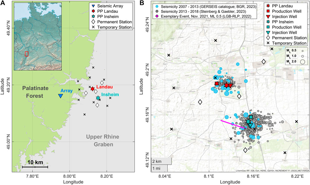
FIGURE 1. Overview of the study area in southwestern Germany. (A) Geological setting with the seismic array (blue triangle) located in the Palatinate Forest and the power plants (PP) Landau (red star) and Insheim (cyan star) located in the Upper Rhine Graben (URG). Stations of the Südpfalz network are distributed within the URG, surrounding both power plants. They include permanent (black diamonds) and temporary (black crosses) installations, operated by the LGB-RLP and the BGR. (B) Seismicity associated with the Landau and Insheim power plants for the period from 2007 to 2018. Events for the years 2007–2013 (blue circles) belong to the GERSEIS database (BGR, 2023). Grey circles show automatized localizations for the period from 2013 to 2018 (Steinberg & Gaebler, 2023). The exemplary event (19 November 2021, M_L 0.5; LGB-RLP, 2022) shown in Figures 3–7 is indicated by the pink circle (see pink arrow).

The Landau and Insheim geothermal power plants are located 4 $km$ apart (cf. Figure 1) and are equipped with boreholes of 3,340 $m$ and 3,800 $m$ depth, respectively (Vasterling et al., 2017). Both power plants are enhanced geothermal systems with fluid injections in different horizons in the transition zone between Mesozoic sediments and crystalline basement (Evans et al., 2012; Vasterling et al., 2017). Groos and Ritter (2014) provide an analysis of the associated seismicity for the years 2006–2013. Küperkoch et al. (2018) detect and locate more than 600 events in the Insheim reservoir between 2013 and 2016. In total, more than 2,200 induced micro-events were detected for the period between 2006 and 2016 (Vasterling et al., 2017). Steinberg and Gaebler (2023) perform re-localizations for events after 2012, using Nonlinloc (Lomax et al., 2000) and a 1-D velocity model (Küperkoch, 2018). We show their results in Figure 1B.

Since 2013, the seismic activity in both reservoirs is monitored by the Federal Institute for Geosciences and Natural Resources (BGR) and the Geological Survey and Mining Authority of Rhineland-Palatinate (LGB-RLP). In addition to the permanent network, a temporary network of seismic stations is operational since 2020 (Südpfalz network). Real-time event detection is implemented using template correlation (Vasterling et al., 2017); localizations are performed manually by the LGB-RLP (LGB-RLP, 2022).

The seismic array was installed in June 2021 in the Palatinate Forest, a small mountain range at the western border of the URG, which is characterized by Buntsandstein formations (e.g., Haneke & Weidenfeller, 2010). The distances to the power plants in Landau and Insheim are 12.5 $km$ and 14 $km$, respectively (cf. Figure 1A). The array includes 10 seismic stations; it has an aperture of 1.1 $km$ (Figure 2) and the maximum distance in elevation between two sites is 71 $m$. The instrumentation includes nine 120 s broadband and one 10 s short-period seismometer. All stations have continuous real-time data streaming of all 3 seismic components (vertical, North, East) at a sampling rate of 200 $Hz$. The average seismic noise level at frequencies of 5–25 $Hz$ is usually below 0.1 $\mu m/s$ ground velocity.

FIGURE 2

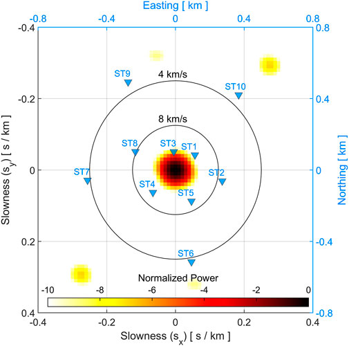
FIGURE 2. Array transfer function and site geometry. The array transfer function is shown in the horizontal ($x$-$y$) plane for a frequency of 10 $Hz$. The locations of the array sites are superimposed (blue triangles, top and right coordinate axes). The array has an aperture of 1.1 $km$.

3 Methods

The slowness vector $\stackrel{\rightharpoonup }{s}$ of a seismic phase, traversing an array as a plane wave, relates the inter-station delay time ${\tau }_{ij}$ to the position vector ${\stackrel{\rightharpoonup }{r}}_{ij}$ (see, e.g., Schweitzer et al., 2012):

${\tau }_{ij}={\stackrel{\rightharpoonup }{r}}_{ij}\bullet \stackrel{\rightharpoonup }{s}=\left(\begin{array}{c}{-x}_{ij}\\ -y_{ij}\\ z_{ij}\end{array}\right)\bullet \left(\begin{array}{c}{s}_x\\ s_y\\ s_z\end{array}\right)=-\frac{x_{ij}\bullet \mathit{sin}\theta }{v_{app,h}}-\frac{y_{ij}\bullet \mathit{cos}\theta }{v_{app,h}}+\frac{z_{ij}}{v_{app,z}}$(1.1)

$\stackrel{\rightharpoonup }{s}=\left(\begin{array}{c}\frac{\sin \theta }{v_{app,h}}\\ \frac{\cos \theta }{v_{app,h}}\\ \frac{1}{v_{app,z}}\end{array}\right)$(1.2)

Here, the position vector ${\stackrel{\rightharpoonup }{r}}_{ij}$ is defined by the spatial distance between two sites $i$ and j ($x_{ij}=x_i-x_j,y_{ij}=y_i-y_j,z_{ij}=z_i-z_j$) and the inverse of the absolute value of the slowness vector equals the average P- or S-wave velocity of the medium beneath the array ($v_c=1/\left|\stackrel{\rightharpoonup }{s}\right|$). In Eq. 1.2, the slowness vector is written in terms of the back azimuth angle (BAZ, $\theta$) and the horizontal and vertical components of $v_c$, referred to as the horizontal and vertical apparent velocity ($v_{app,h}$ and $v_{app,z}$), respectively.

Most array processing techniques estimate the slowness vector in the horizontal plane exclusively. This requires an array setup with marginal differences in elevation. Schweitzer et al. (2012) state that elevation correction factors should be applied if deviations in time delay become larger than ¼ of the dominant signal period. These correction terms involve assumptions about the usually unknown subsurface velocity beneath the array ($v_c$) and the vertical incidence angle $i=\mathrm{atan}\left(v_{app,z}/v_{app,h}\right)$.

A common procedure to estimate the wavefront parameters $\theta$ and $v_{app,h}$ relates to a maximization of the beam power in the horizontal slowness plane ${\stackrel{\rightharpoonup }{s}}_h=\left({\stackrel{\rightharpoonup }{s}}_x,{\stackrel{\rightharpoonup }{s}}_y\right)$. Applying Parseval’s theorem, the beam energy $E\left(k\right)$ is defined as (e.g., Kelly, 1967):

$E\left(\stackrel{\rightharpoonup }{k}-{\stackrel{\rightharpoonup }{k}}_0\right)=\frac{1}{2\pi }{\int }_{-\infty }^{\infty }{\left|S\left(\omega \right)\right|}^2{\left|\frac{1}{N}{\displaystyle \sum _{j=1}^N}{e}^{2\pi i{\left(\stackrel{\rightharpoonup }{k}-{\stackrel{\rightharpoonup }{k}}_{\mathbf{0}}\right)\stackrel{\rightharpoonup }{r}}_j}\right|}^{2}d\omega$(2.1)

where $S\left(\omega \right)$ is the Fourier transform of the signal at site $j$, ${\stackrel{\rightharpoonup }{r}}_j$ the position vector of site $j$, $N$ the number of sites in the array and $\omega$ the angular frequency. The vectors $\stackrel{\rightharpoonup }{k}={\stackrel{\rightharpoonup }{s}}_h\omega$ and ${\stackrel{\rightharpoonup }{k}}_0={\stackrel{\rightharpoonup }{s}}_{h,0}\omega$ are wavenumber vectors, defined by the unknown horizontal slowness vector ${\stackrel{\rightharpoonup }{s}}_{h,0}$ of the plane wave and the horizontal beam steering vector ${\stackrel{\rightharpoonup }{s}}_h$. The second squared term of the integrand in (2.1) defines the array response function:

${\left|A\left(k-k_0\right)\right|}^2={\left|\frac{1}{N}{\displaystyle \sum _{j=1}^N}{e}^{2\pi i\left(\stackrel{\rightharpoonup }{k}-{\stackrel{\rightharpoonup }{k}}_{\mathbf{0}}\right){\stackrel{\rightharpoonup }{r}}_j}\right|}^2$(2.2)

The array response function characterizes the array pattern in the wavenumber space at a given frequency. In Figure 2 it is shown for the array in the Palatinate Forest, for a slowness range from −0.4 to 0.4 $s/km$ and a frequency of 10 $Hz$.

Eq. 2.1 can be evaluated over a grid in the horizontal slowness plane, where the location of the energy maximum provides an estimate for the back azimuth and horizontal apparent velocity of the incident plane wave. The method is referred to as frequency-wavenumber (f-k) analysis.

In our work, we use observed inter-station delay times to estimate the slowness vector $\stackrel{\rightharpoonup }{s}$ from Eq. 1.1 using linear regression (Del Pezzo & Giudicepietro, 2002; Szuberla & Olsen, 2004 or Olsen & Szuberla, 2005). This requires an accurate estimation of the delay times and a reliable and robust regression approach, which is addressed in detail in the following sections.

3.1 Delay time estimation

We use a normalized cross-correlation function to obtain estimates for the delay times related to an incoming seismic wavefront (e.g., Claerbout, 1986; Olsen & Szuberla, 2005). The normalized cross correlation-function ($\rho$) for two signals $A_i\left(t_0\right)=〈A_{i,t_0-K/2:t_0+K/2}〉$ and $A_j\left(t_0\right)=〈A_{j,t_0-K/2:t_0+K/2}〉$ with length $K$ and centered at the time $t_0$, is defined as dependent on the time shift $t$ between the signals (e.g., Claerbout, 1986):

${\rho \left(t_0,t\right)}_{A_i,A_j}=\frac{E\left[\left(A_i\left(t_0\right)-\mu \left[A_i\left(t_0\right)\right]\right){\left(A_j\left(t_0-t\right)-\mu \left[A_j\left(t_0\right)\right]\right)}^{*}\right]}{\sigma \left[A_i\left(t_0\right)\right]\sigma \left[A_j\left(t_0\right)\right]}(3)$

with $E$ being the expected value, the asterisk (*) denoting the complex conjugate, and $\mu$ and $\sigma$ defining the mean and standard deviation of $A_i$ and $A_j$, respectively. In practice, Eq. 3 can be solved either in the time- or in the frequency-domain.

The travel time difference (delay time, $\tau$) of a seismic phase, recorded at two points of observation, is then given by the argument of the maximum ($\mathit{argmax}$) of $\rho \left(t_0,t\right)$ within a predefined time shift interval $t=〈t_0-\Delta t:t_0+\Delta t〉$ of the two signals. Here, the choice of the maximum time shift $\Delta t$ should account for the aperture of the array and the minimum of the apparent velocity range of interest. In our case we choose $\Delta t=0.5s$, which is appropriate for an aperture of $1.1km$ and a minimum $v_{app,h}$ of $2.2km/s$.

The function $\rho \left(t_0,t\right)$ can be evaluated for all pairs of array stations ($A_{i=1:N}$ and $A_{j=1:N}$, with $N$ being the number of sites), resulting in a cross-correlation matrix $\mathit{C}$ of the seismic signal at the time $t_0$:

$\mathit{C}\left(t_0\right)=\left[\mathit{max}\left({\rho \left(t_0,t\right)}_{A_i=1:N,A_j=1:N}\right)\right]=\left[\begin{array}{ccc}\mathit{max}\left({\rho \left(t_0,t\right)}_{A_1,A_1}\right)& \dots & \mathit{max}\left({\rho \left(t_0,t\right)}_{A_1,A_N}\right)\\ ⋮& \ddots & ⋮\\ \mathit{max}\left({\rho \left(t_0,t\right)}_{A_N,A_1}\right)& \dots & \mathit{max}\left({\rho \left(t_0,t\right)}_{A_N,A_N}\right)\end{array}\right]$(4.1)

The associated delay time vector $\stackrel{\rightharpoonup }{\tau }$ forms the basis for our further analysis.

$\stackrel{\rightharpoonup }{\tau }\left(t_0\right)=\left[\mathit{argmax}\left({\rho \left(t_0,t\right)}_{A_i=1:N,A_j=1:N;i\ne j}\right)\right]=\begin{array}{c}\mathit{argmax}\left({\rho \left(t_0,t\right)}_{A_1,A_1}\right)\\ ⋮\\ \mathit{argmax}\left({\rho \left(t_0,t\right)}_{A_N,A_N}\right)\end{array}$(4.2)

Eqs. 3, 4 are evaluated in fixed time steps, which results in continuous functions of the median cross correlation matrix $\mathit{C}$ and the delay time vector $\stackrel{\rightharpoonup }{\tau }$ (and subsequently back azimuth, and horizontal apparent velocity), with time $t0$. In our case, we use a temporal resolution of 10 samples (0.05 $s$). The values of the time dependent cross-correlation matrix further provide useful parameters for event detection (Smith & Bean, 2020). We suggest using the median as a robust estimator of the mean of $\mathit{C}\left(t0\right)$, which must exceed a defined threshold (${\rho }_{\mathit{min}}$):

$MC\left(t0\right)=median\left({\mathit{C}\left(t0\right)}_{A_i\ne A_j}\right)>{\rho }_{\mathit{min}}(5)$

The choice of ${\rho }_{\mathit{min}}$ depends on the local noise conditions, the subsurface characteristics beneath the array sites, and on the size of the correlation window. In our case, ${\rho }_{\mathit{min}}=0.4$ proves to be a good trade-off to maintain the sensitivity to earthquakes with small magnitudes while minimizing the number of false detections. It is important to note that at this stage, the term event does not imply a defined source of the signal (e.g., induced/natural earthquake or correlated seismic noise). This is different to, e.g., Vasterling et al. (2017), who use a continuous correlation with master events to detect seismicity in the reservoirs.

Figure 3 demonstrates the principles of the method for an exemplary event from the Insheim reservoir, recorded on 19 November 2021. It has a local magnitude (M_L) of 0.5 and the network localization involves a theoretical back azimuth angle of 97.5° at the array (see Figure 3A). The time series (Figure 3B) are band pass filtered (between 5 Hz and 25 Hz) and a 1.5 $s$ time window is used for the correlation analysis. Results are shown for six different site combinations in terms of their normalized cross-correlation functions ($\left.\rho \left(t_0,t\right)\right)$ and the corresponding delay times (see Figure 3C), for a time window centered at the point of maximum correlation $\left(\mathit{argmax}\left(MC\right)\right.$). The plane wavefront traverses the array from east to west (BAZ 97.5°), resulting in large delay times for station pairs with significant location differences in east-west direction.

FIGURE 3

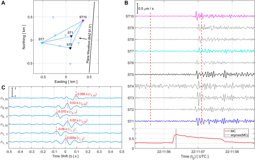
FIGURE 3. Delay time estimation for an exemplary event from the Insheim reservoir (M_L 0.5, BAZ to network localization: 97.5°). (A) Station geometry and orientation of the plane wavefront. The colored sites are used to calculate the cross-correlation functions in C. (B) Waveforms of the vertical (Z) component from all 10 array sites, displaying the P-wave onsets. The waveforms are band-pass filtered between 5 and 25 $Hz$. The dashed red lines show the limits of the 1.5 $s$ correlation window used in C. The position is defined by the point of maximum correlation (dotted black line) determined by the median of the cross-correlation matrix ($MC)$, which is shown in the bottom. (C) Normalized cross-correlation function for six inter-station pairs (${\rho }_{A_i,A_j}$) calculated at $\mathit{argmax}\left(MC\right)$. The dashed red lines mark the arguments of the maxima of ${\rho }_{A_i,A_j}$ which give estimates for the delay times (${\tau }_{i,j}$). All delay times are given with reference to the station indicated by the second index (${\tau }_{\mathrm{7,10}}$, for example, implies that the wavefront reaches ST7 0.095 $s$ after ST10).

The normalized cross-correlation function in Equation 3 performs well for adequate signal to noise conditions, but outliers in single observations can significantly bias subsequent calculations. We therefore recommend using a continuous evaluation of the median of the cross-correlation matrix ($MC$) as a robust trigger function (bottom Figure 3B). This function (usually) takes a maximum when the correlation window includes the P-wave onsets but excludes the P-wave coda (cf. Figure 3B, dashed red and black lines). It remains unaffected by correlated noise between single station pairs or degraded signal to noise conditions at individual sites. If a set of observed delay times includes outliers, the use of robust array processing techniques will be essential (see section 3.2.1 and supplements).

3.2 Estimating the full 3-D slowness vector using linear regression

Del Pezzo and Giudicepietro (2002) and Olsen and Szuberla (2005) use a linear regression model to fit a vector of inter-station delay times ($\stackrel{\rightharpoonup }{\tau }$) and obtain estimates for the horizontal slowness vector ${\stackrel{\rightharpoonup }{s}}_h$. The concept can be extended to account for differences in elevation:

$\stackrel{\rightharpoonup }{\tau }=\left(\begin{array}{c}{\tau }_1\\ ⋮\\ {\tau }_n\end{array}\right)=-\stackrel{\rightharpoonup }{x}{s}_x-\stackrel{\rightharpoonup }{y}{s}_y+\stackrel{\rightharpoonup }{z}{s}_z+\stackrel{\rightharpoonup }{ϵ}$

$=\left(\begin{array}{ccc}{-x}_1& {-y}_1& z_1\\ ⋮& ⋮& ⋮\\ {-x}_n& {-y}_n& z_n\end{array}\right)\bullet \left(\begin{array}{c}{s}_x\\ s_y\\ s_z\end{array}\right)+\left(\begin{array}{c}{ϵ}_1\\ ⋮\\ {ϵ}_n\end{array}\right)=\mathit{X}\stackrel{\rightharpoonup }{s}+\stackrel{\rightharpoonup }{ϵ}(6)$

where $n$ is the number of independent observations in the regression model, $\stackrel{\rightharpoonup }{x}$, $\stackrel{\rightharpoonup }{y}$ and $\stackrel{\rightharpoonup }{z}$ are inter-station distance and elevation difference vectors, $\stackrel{\rightharpoonup }{ϵ}$ includes the unknown error terms and the matrix $\mathit{X}$ is the design matrix, defined by the predictor variables. The full 3-D slowness vector $\stackrel{\rightharpoonup }{s}$ corresponds to the coefficient (or parameter) vector of the regression model.

The solution of the regression model is crucial to get accurate parameter estimates. M-estimators (maximum likelihood-type; Huber, 1981) provide a broad class of extremum estimators and allow for the inclusion of robust statistics (see section 3.2.1). They are a generalization of the objective function in L1- (least absolute deviation) and L2-norm (least squares) regression and estimate the maximum of the likelihood function for a parameter vector $\stackrel{\rightharpoonup }{s}$ and a sample distribution $\chi$ with probability density function $f\left(\chi \right)=C{e}^{-\sigma \left(\chi \right)}$ (Bishop et al., 2020, following Rousseeuw & Leroy 1987). The solution is usually implemented as a minimization of a cost function (Huber, 1981):

$\stackrel{\rightharpoonup }{\widehat{s}}=\begin{array}{c}\mathit{argmin}\\ \stackrel{\rightharpoonup }{s}\end{array}\left({\displaystyle \sum _{i=1}^n}\sigma \left({ϵ}_i\left(\stackrel{\rightharpoonup }{s}\right)\right)\right)(7)$

Here, $\sigma$ is a symmetric function of the regression residuals ${ϵ}_i\left(\stackrel{\rightharpoonup }{s}\right)$, which has a unique zero (Bishop et al., 2020; following Huber, 1973). In Eq. 6, the sample distribution $\chi$ is given by the design matrix $\mathit{X}$ and the minimization problem can be written as:

$\stackrel{\rightharpoonup }{\widehat{s}}=\begin{array}{c}\mathit{argmin}\\ \stackrel{\rightharpoonup }{s}\end{array}\left({\displaystyle \sum _{i=1}^n}\sigma \left({\tau }_i-{\mathit{X}}_i\stackrel{\rightharpoonup }{s}\right)\right)(8)$

With ${\mathit{X}}_i$ and ${\tau }_i$ being the $i$ th row of $\mathit{X}$ and the $i$ th component of the delay time vector $\stackrel{\rightharpoonup }{\tau }$, respectively. The estimated parameter vector $\stackrel{\rightharpoonup }{\widehat{s}}$ minimizes the cost function and predicts the slowness vector of the incident plane wave.

If the errors in $\stackrel{\rightharpoonup }{ϵ}$ are normally distributed, the least squares estimator ($\sigma ={\left|{ϵ}_i\left(\stackrel{\rightharpoonup }{s}\right)\right|}^2$) recovers the optimum parameter vector that minimizes the squared residuals. The ordinary least squares (OLS) formulation assumes a linear relation between response and predictor variables. It is given as (see, e.g., Lai et al., 1978):

$\stackrel{\rightharpoonup }{\widehat{s}}={\left({\mathit{X}}^T\mathit{X}\right)}^{-1}{\mathit{X}}^T\stackrel{\rightharpoonup }{\tau }(9)$

where $T$ denotes the transpose of a matrix. Eq. 9 has a unique solution if the matrix $\mathit{X}$ is full rank.

The deviation between observed ($\stackrel{\rightharpoonup }{\tau })$ and predicted ($\stackrel{\rightharpoonup }{\widehat{\tau }}=\mathit{X}\stackrel{\rightharpoonup }{\widehat{s}}$) delay times defines the root mean squared error ($RMSE$) of the regression model:

$RMSE\left(\stackrel{\rightharpoonup }{\tau }\right)=\sqrt{\frac{{\displaystyle \sum _{i=1}^n}{\left({\tau }_i-{\widehat{\tau }}_i\right)}^2}{n-p}}(10)$

with $p$ being the number of independent predictor variables (here three). Further, the coefficient variances and covariances are calculated from the mean squared error ($MSE={RMSE\left(\stackrel{\rightharpoonup }{\tau }\right)}^2$) of the dependent variable and the inverse covariance matrix of the predictor variables:

$\mathit{C}\mathit{o}\mathit{v}\left(\widehat{s}\right){{=RMSE\left(\tau \right)}^2\left({\mathit{X}}^T\mathit{X}\right)}^{-1}=\left(\begin{array}{ccc}{{\sigma }_{\widehat{s}x}}^2& {{\sigma }_{\widehat{s}x,y}}^2& {{\sigma }_{\widehat{s}x,z}}^2\\ {{\sigma }_{\widehat{s}y,x}}^2& {{\sigma }_{\widehat{s}y}}^2& {{\sigma }_{\widehat{s}y,z}}^2\\ {{\sigma }_{\widehat{s}z,x}}^2& {{\sigma }_{\widehat{s}z,y}}^2& {{\sigma }_{\widehat{s}z}}^2\end{array}\right)(11)$

The square-root of the diagonal variances are the standard errors of the regression coefficients (${\sigma }_{\widehat{s}x}$, ${\sigma }_{\widehat{s}y}$ and ${\sigma }_{\widehat{s}z}$). They can be used to derive confidence intervals (CI; e.g., Wald, 1943):

$\left(\begin{array}{c}\begin{array}{c}\mathrm{C}\mathrm{I}\left({\widehat{s}}_x\right)\\ \mathrm{C}\mathrm{I}\left({\widehat{s}}_y\right)\end{array}\\ \mathrm{C}\mathrm{I}\left({\widehat{s}}_z\right)\end{array}\right)=\mathrm{t}\_\mathrm{d}\mathrm{i}\mathrm{s}\mathrm{t}\left(1–\frac{\mathrm{\alpha }}{2},\mathrm{n}–\mathrm{p}\right)\bullet \left(\begin{array}{c}\begin{array}{c}{\sigma }_{\widehat{s}x}\\ {\sigma }_{\widehat{s}y}\end{array}\\ {\sigma }_{\widehat{s}z}\end{array}\right)(12)$

where $t\_dis{t}_{\left(1–\alpha /2,n–p\right)}$ is the $100\left(1–\alpha /2\right)$ percentile of the t-distribution with $n–p$ degrees of freedom. For the 95% confidence interval (significance level $\alpha =0.05$) and 87 degrees of freedom, $t\_dist$ takes a value of 1.9913 (see any statistical table for the t-distribution).

The back azimuth angle $\theta$ and the horizontal and vertical apparent velocity ($v_{app,h}$ and $v_{app,z}$) of the plane wave can be calculated from the components of the estimated slowness vector:

$\theta =\mathit{atan}2\left({\widehat{s}}_x,{\widehat{s}}_y\right)$(13.1)

$v_{app,h}=\sqrt{\frac{1}{{{\widehat{s}}_x}^2+{{\widehat{s}}_y}^2}}$(13.2)

$v_{app,z}=\frac{1}{{\widehat{s}}_z}$(13.3)

We calculate the associated errors using error propagation (see Szuberla & Olsen, 2004; De Angelis et al., 2020), neglecting the coefficient co-variances, which are in average ten times smaller than the variances. This follows the assumption of uncorrelated errors in the predictor variables.

$\sigma \theta =\sqrt{{\left(\frac{{\widehat{s}}_y}{{{\widehat{s}}_x}^2+{{\widehat{s}}_y}^2}{\sigma }_{\widehat{s}x}\right)}^2+{\left(-\frac{{\widehat{s}}_x}{{{\widehat{s}}_x}^2+{{\widehat{s}}_y}^2}{\sigma }_{\widehat{s}y}\right)}^2}$(14.1)

$\sigma v_{app,h}=\sqrt{{\left(-\frac{{\widehat{s}}_x}{{\left({{\widehat{s}}_x}^2+{{\widehat{s}}_y}^2\right)}^{3/2}}{\sigma }_{\widehat{s}x}\right)}^2+{\left(-\frac{{\widehat{s}}_y}{{\left({{\widehat{s}}_x}^2+{{\widehat{s}}_y}^2\right)}^{3/2}}{\sigma }_{\widehat{s}y}\right)}^2}$(14.2)

$\sigma v_{app,z}=\frac{1}{{{\widehat{s}}_z}^2}{\sigma }_{\widehat{s}z}$(14.3)

Figure 4 shows regression results for the exemplary event from the Insheim reservoir, with delay times $\stackrel{\rightharpoonup }{\tau }$ obtained at the point of maximum correlation ($\mathit{arg}\mathit{max}\left(MC\right)$, cf. Figure 3). The regression model reveals a strong dependence in east-west ($x$) direction, whereas the dependence in north-south ($y$) direction seems much smaller (see Figure 4A). Figure 4B examines the effect of the predictor variables $\stackrel{\rightharpoonup }{x}$, $\stackrel{\rightharpoonup }{y}$ and $\stackrel{\rightharpoonup }{z}$ on the regression result through partial regression leverage plots (see, e.g., Velleman & Welsch, 1981). It shows that most of the observed delay time (adjusted $\tau$) is covered by variations in $\stackrel{\rightharpoonup }{x}$; the influences from $\stackrel{\rightharpoonup }{y}$ and $\stackrel{\rightharpoonup }{z}$ are comparable. At the same time, the three regression coefficients (${\widehat{s}}_x$ ${\widehat{s}}_y$, and ${\widehat{s}}_z$) clearly reject the null-hypothesis at a significance level of 0.05 ($p<0.001$), which indicates a substantial contribution to the regression results for all spatial coordinates. However, the standard errors of the regression coefficients reveal that uncertainties within the vertical component of the slowness vector (${\widehat{s}}_z$) are by a factor of ten larger if compared to the horizontal components (0.065 $s/km$ for ${\widehat{s}}_z$, 0.005 $s/km$ for ${\widehat{s}}_x$ and ${\widehat{s}}_y$). This is a consequence of the much smaller variance in elevation in comparison to the horizontal inter-station distances (cf. Eq. 11). The estimated 3-D slowness vector and the corresponding 95% confidence ellipsoid are visualized in Figure 4C.

FIGURE 4

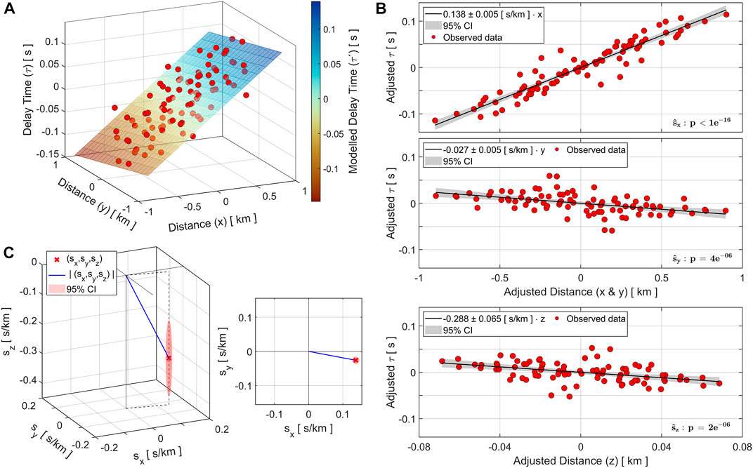
FIGURE 4. Estimation of the full slowness vector using least squares regression. (A) The red circles show the observed delay times for the exemplary event in the Insheim reservoir (M_L 0.5, BAZ to network localization: 97.5°), plotted against the horizontal inter-station distances ($\stackrel{\rightharpoonup }{x}$ and $\stackrel{\rightharpoonup }{y}$). The plane shows the regression model for the horizontal coefficients (${\widehat{s}}_x$ and ${\widehat{s}}_y$), the color indicates the modelled/predicted delay time. (B) Partial regression leverage plots for the three independent variables ($\stackrel{\rightharpoonup }{x}$, $\stackrel{\rightharpoonup }{y}$ and $\stackrel{\rightharpoonup }{z}$). $\stackrel{\rightharpoonup }{x}$ contributes most to the model, but the contributions from $\stackrel{\rightharpoonup }{y}$ and $\stackrel{\rightharpoonup }{z}$ are statistically significant. (C) Visualization of the estimated slowness vector in 3-D (left) and in the horizontal plane (right). The 95% confidence ellipsoid shows that uncertainties in the vertical direction are much larger compared to the horizontal directions.

Our results show that the inclusion of elevation differences in the regression model allows for an estimation of the vertical slowness component ($s_z$). However, in our case, the maximum difference in elevation is 71 $m$, which is less than one-fifteenth of the maximum horizontal extension. Therefore, the statistical uncertainties of the results must be evaluated with caution.

3.2.1 Robustness

Outliers in the response and predictor variables can significantly bias ordinary least squares regression and require careful consideration. The statistical definition of an outlier refers to observations that deviate significantly from other members of the underlying data distribution (e.g., Grubbs, 1969 or Rousseuw, 1984). In case of seismic arrays, outliers are delay time observations that are inconsistent with the plane wave model (Bishop et al., 2020). They can relate to a low signal to noise ratio at one or multiple sites, timing errors (clock drift or failure) or strong subsurface distortion at individual sites.

The effects from outliers on linear regression are well studied and robust estimators are designed to weaken or eliminate their influence (e.g., Rousseeuw & Leroy 1987). We tested and compared the performance of a Biweight M-estimator, implemented via iteratively reweighted least squares (IRLS), and least trimmed squares (LTS) regression (see Supplementary Text S1, Supplementary Figure S1 and Supplementary Figure S2 for details). The results show that the Biweight M-estimator yields stable and consistent results for BAZ and apparent velocity, even for large quantities of outliers (>25%). IRLS proves to be particularly well suited, as it diminishes effects from outliers by dragging them towards a normal distribution, whilst the parameter estimates are still defined by the mean of the data. Here, the algorithm minimizes the exclusion of data. In this regard it is similar to the limited sensor pair correlation approach (Gibbons et al., 2018), which improves the robustness of an f-k analysis by excluding weakly correlated sensor pairs.

Our implementation of the Biweight M-estimator follows Beaton and Tukey (1974), Holland and Welsch (1977) and Du Mouchel and O’Brien (1989). It adds a weighting term ($w$) to the error function ($\sigma$) in Equation 7 (e.g.; Huber, 1981):

$\stackrel{\rightharpoonup }{\widehat{s}}=\begin{array}{c}\mathit{argmin}\\ \stackrel{\rightharpoonup }{s}\end{array}\left({\displaystyle \sum _{i=1}^n}\sigma \left({w_i\left(\stackrel{\rightharpoonup }{s}\right)ϵ}_i\left(\stackrel{\rightharpoonup }{s}\right)\right)\right)(15)$

There is no analytical solution to this equation and we use a reweighted least squares algorithm (Beaton & Tukey, 1974) to iteratively adjust the weighting function. The algorithm starts from an ordinary least squares regression ($w=1$) and successively reweights observations causing untypically large residuals. For every iteration and each observation $i$, weights ($w_i$) are calculated using the Biweight function (Beaton & Tukey, 1974; Holland & Welsch, 1977):

$w_i=\left\{\begin{array}{c}{\left(1-{r_i}^2\right)}^2,\left|r_i\right|<1\\ 0,\left|r_i\right|\ge 1\end{array}\right.$(16.1)

with $r_i$ being the standardized adjusted residuals, calculated from the residuals ${ϵ}_i$ and the leverage values $h_i$ of the previous iteration:

$r_i=\frac{{ϵ}_i}{tc\bullet rs\bullet \sqrt{1-h_i}}$(16.2)

Here, the leverage values $h_i$ are defined as the diagonal elements of the projection matrix $\mathit{H}={\mathit{X}\left({\mathit{X}}^T\mathit{W}\mathit{X}\right)}^{-1}{\mathit{X}}^T\mathit{W}$, where $\mathit{W}$ defines the diagonal weight matrix. The term $rs=1.483MAD$ is a robust estimate of scale, derived as the median absolute deviation ($MAD$) of the residuals from their median, and with the value $1.483$ related to the inverse of the cumulative distribution function. It makes the estimate unbiased for a normal distribution (see, e.g., Rousseeuw & Leroy, 1987). The factor $tc$ is a tuning constant, where smaller values result in stronger down-weighting of outliers (we chose $tc=3$).

The solution of the weighted least squares problem is defined as:

$\stackrel{\rightharpoonup }{\widehat{s}}={\left({\mathit{X}}^T\mathit{W}\mathit{X}\right)}^{-1}{\mathit{X}}^T\mathit{W}\stackrel{\rightharpoonup }{\tau }(17)$

After each iteration, the loss function from Eq. 15 is evaluated:

$l\left(\stackrel{\rightharpoonup }{\widehat{s}}\right)={\displaystyle \sum _{i=1}^n}\sigma ({w_i\left(\stackrel{\rightharpoonup }{\widehat{s}}\right)ϵ}_i\left(\stackrel{\rightharpoonup }{\widehat{s}}\right))={\displaystyle \sum _{i=1}^n}\sigma \left(w_i\left(\stackrel{\rightharpoonup }{\widehat{s}}\right)\left({\tau }_i-{\mathit{X}}_i\stackrel{\rightharpoonup }{\widehat{s}}\right)\right)(18)$

The algorithm stops if the solution converges or if the iteration limit is reached. We chose the loss function $\sigma$ to be a type L2-normalization ($\sigma ={\left|w_i\left(\stackrel{\rightharpoonup }{\widehat{s}}\right){ϵ}_i\left(\stackrel{\rightharpoonup }{\widehat{s}}\right)\right|}^2$), however, it can also contain a least absolute deviation model (L1-norm, $\sigma =\left|{w_i\left(\stackrel{\rightharpoonup }{\widehat{s}}\right)ϵ}_i\left(\stackrel{\rightharpoonup }{\widehat{s}}\right)\right|$).

3.3 Comparison of methods

In this section, we compare results from iteratively reweighted least squares (IRLS) and ordinary least squares (OLS) regression to the widely used frequency-wavenumber (f-k) analysis (Capon, 1969). The performance and stability of an f-k analysis highly depends on the applied frequency band (see, e.g., Kværna & Ringdal, 1986 or Kværna & Doornbos, 1991). Generally, the application of suitable, fixed frequency bands is supposed to yield superior results in comparison to a wide-frequency band approach (Gibbons et al., 2005). At the same time, the width of the adapted frequency bands is crucial and should not be too small (Kværna & Ringdal, 1986; Gibbons et al., 2010).

We calculate the energy of the array beam according to Eq. 2.1 for a slowness-grid in the range from −0.4 to 0.4 $s/km$ and with a resolution of 0.01 s/km. The fixed time window length is 1.5 $s$ (identical to the regression approaches). The data are band-pass filtered and tapered prior to the transformation in the frequency domain.

Figure 5 evaluates the performance and stability of the OLS and IRLS regression methods and compares them to frequency-wavenumber analysis. Figure 5A shows the time dependent cross-correlation function for the exemplary event from the Insheim reservoir (M_L 0.5, BAZ network localization: 97.5°). Figure 5B compares results for back azimuth and horizontal apparent velocity depending on the shift relative to the point of maximum correlation. It shows that the results are generally unreliable for negative time shifts. In this case, the analysis window does not include enough signal component (cf. Position of the time window at $\mathit{argmax}\left(MC\right)$ in Figure 3B). However, for positive time shifts, IRLS regression yields reliable and consistent values, not much influenced by the position of the time window. OLS regression is stable up to a $\mathit{argmax}\left(MC\right)$ + 0.4 s. The f-k results, on the other hand, are unstable and only partially reliable (e.g., at $\mathit{argmax}\left(MC\right)$ + 0.15 s). Figure 5C examines the frequency band parameters for the f-k analysis with a correlation window shifted by 0.15 $s$ from $\mathit{argmax}\left(MC\right)$. It shows that the results heavily rely on the frequency band. In this case, the band between 5 and 11 Hz (8 Hz ± 3 Hz) is preferable (BAZ closest to the network localization); however, this conclusion cannot be generalized. The optimal settings can vary significantly depending on the position of the time window and on the source field and ray paths characteristics of the signal (Kværna & Doornbos, 1991). Figure 5D shows the energy grid of the f-k analysis at $\mathit{argmax}\left(MC\right)+0.15s$, derived for optimized frequency settings (8 Hz ± 3 Hz). The energy maximum is close to the results from IRLS and OLS regression, but there is a nearby secondary maximum, which indicates an instability of the solution. In comparison to the network localization, the back azimuth of the f-k analysis is slightly too small. The deviation most likely relates to the neglection of elevation differences between the array sites. If the regression approaches are restricted to the horizontal plane, the resulting back azimuth is similar to the f-k result.

FIGURE 5

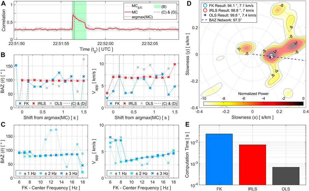
FIGURE 5. Comparison of processing methods for the exemplary event (M_L 0.5, BAZ to network localization: 97.5°). (A) Median of the cross-correlation matrix ($MC$) for all sites (red line) and for the individual sites (grey lines). The black dotted line indicates the point of maximum correlation ($\mathit{argmax}\left(MC\right)$). The green area encloses the center positions of the 1.5 $s$ correlation windows used in B, while the black dashed line shows the position in C and D. (B) Results for BAZ (left) and $v_{app,h}$ (right) in dependence on the shift relative to the point of maximum correlation, for the IRLS and OLS estimators, and the f-k analysis. The frequency band for the f-k analysis is 5–11 $Hz$. IRLS results are very stable and consistent. The f-k solutions are only partly reliable (e.g., at $\mathit{argmax}\left(MC\right)+0.15\mathrm{s}$) and differ dramatically. (C) Results for BAZ (left) and $v_{app,h}$ (right) for different center frequencies and bandwidths in the f-k analysis. The correlation window is centered at $\mathit{argmax}\left(MC\right)+0.15\mathrm{s}$. (D) Energy grid of the f-k analysis (window at $\mathit{argmax}\left(MC\right)+0.15\mathrm{s}$, frequency band: 5–11 $Hz$). The maximum is indicated by the blue circle. Results from the IRLS and OLS regressions and the BAZ of the network localization are included for comparison. (E) Computation time for the IRLS, OLS and f-k analysis, measured on a modern desktop computer (logarithmic timescale). For the regression approaches, the computation time includes the delay time estimations using inter-station cross correlation functions.

The computation time is of great relevance regarding real-time applications. It is compared for all three approaches using a modern desktop computer (Figure 5E). All methods take less than 0.1 s for one calculation. However, OLS regression is almost 50 times and IRLS approximately 4 times faster if compared to an f-k analysis. Considering that IRLS results are significantly more stable than OLS, the IRLS algorithm appears to be a good trade-off between computational efficiency and accuracy, which makes it an excellent choice for real-time application.

3.4 Distance estimation

The determination of P- and S-wave arrival times is a key task in localizing earthquakes. Many current approaches apply deep learning algorithms, which perform very efficient in real-time applications, but require extensive training data sets (usually 10th of thousands of events, e.g., Mousavi et al., 2020 or Li et al., 2022). Another well-established method is the autoregressive Akaike-Information-Criterion (AR-AIC; e.g., Sleeman and Van Eck, 1999), which uses autoregressive filtering to estimate the wave onset as a maximization of the likelihood function in dependence of the division point between two locally stationary signal segments.

Here, we apply a statistical changepoint approach, which, similar to the AC-AIC, divides a time series signal into two locally stationary segments and evaluates a global statistical parameter for each part (see, e.g., Sen & Srivastava, 1975; Chen & Gupta, 2001 or Shi et al., 2022). The changepoint is then derived through a minimization of a loss function, defined by the residuals from the individual samples with reference to the global parameters.

For decent signal to noise ratios, the onset of a seismic signal usually involves an increase in the signal’s standard deviation. Assuming a time series $x_{j,t}=〈x_{j,1:K}〉$ at site $j$ and with length $K$, a function (${CPF}_j$) can be formulated in dependence on the division point $t_k$:

${CPF}_j\left(t_k\right)={\displaystyle {\sum }_{t=1}^{t_k}}\left|x_{j,t}-std\left(〈x_{j,1:t_k}〉\right)\right|+{\displaystyle {\sum }_{t=t_k+1}^K}\left|x_{j,t}-std\left(〈x_{{j,t}_k+1:K}〉\right)\right|(19)$

The signal onset $T_{\left\{P,S\right\},j}$ is then defined for the point $t_k$ that minimizes (19)

$T_{\left\{P,S\right\},j}=\begin{array}{c}\mathit{argmin}\\ t_k\end{array}\left({\displaystyle {\sum }_{t=1}^{t_k}}\left|x_{j,t}-std\left(〈x_{j,1:t_k}〉\right)\right|+{\displaystyle {\sum }_{t=t_k+1}^K}\left|x_{j,t}-std\left(〈x_{{j,t}_k+1:K}〉\right)\right|\right)$(20.1)

and simultaneously fulfills

${\displaystyle {\sum }_{t=1}^{t_k}}\left|x_{j,t}-std\left(〈x_{j,1:t_k}〉\right)\right|+{\displaystyle {\sum }_{t=t_k+1}^K}\left|x_{j,t}-std\left(〈x_{{j,t}_k+1:K}〉\right)\right|<{\displaystyle {\sum }_{t=1}^K}\left|x_{j,t}-std\left(〈x_{j,1:K}〉\right)\right|$(20.2)

i.e., the introduction of a changepoint must improve the cost function. We implement the cost function as a least absolute deviation model (a L1-normalization), which is usually less sensitive to outliers if compared to least squares. Equation 20.1 can be solved by a penalized likelihood approach (see Yao, 1988 or Chen and Gupta, 1997) and the application of a suitable information criterion (here, Bayesian Information Criterion, BIC). The method can be generalized to search for multiple changepoints using, e.g., binary segmentation (Sen & Srivastava, 1975), the segmented neighborhood approach (Auger and Lawrence, 1989), or the OP and PELT methods (Jackson et al., 2005; Killik et al., 2012). For a scenario where the approximate travel time difference between P- and S-wave is predictable (e.g., when monitoring reservoirs), it is more efficient to apply two single changepoint searches within appropriate time windows. In general, the search for a statistical changepoint can be extended to the spectral domain (e.g., Picard, 1985), which might yield improved results for limited signal to noise conditions.

Similar to the AR-AIC, the determination of wave onsets using changepoint analysis depends on an initial estimate of the P-wave arrival. Here, the maximum of the median of the cross-correlation function ($\mathit{argmax}\left(MC\right)$) provides a suitable reference point. For the P-wave arrival we choose a 3.5 $s$ time window, starting at $\mathit{argmax}\left(MC\right)-0.5s$. The window for the S-wave arrival starts 0.5 $s$ after the estimated P-wave arrival and has a length of 5 $s$. Equations 20.1 and 20.2 are evaluated for all $N$ array sites, using the vertical and horizontal components for the P- and S-wave arrivals, respectively. The individual arrival times are subsequently corrected for the inter-station delay times, derived from the array analysis, and a robust estimate for $T_{\left\{P,S\right\}}$ is calculated as:

$T_{\left\{P,S\right\}}=median\left(〈T_{\left\{P,S\right\},1:N}〉\right)(21)$

The median absolute deviation of the individual arrival times from their median is used for error estimation (Hampel, 1986):

${\delta T}_{\left\{P,S\right\}}=1.483\bullet \frac{median\left|〈T_{\left\{P,S\right\},1:N}-median\left(〈T_{\left\{P,S\right\},1:N}〉\right)〉\right|}{\sqrt{N}}(22)$

where the value $1.483$ relates to the inverse of the 0.75th quantile of the cumulative distribution.

Figures 6A, B show continuous evaluations of ${CPF}_j$ (Eq. 19) within fixed time windows, for the vertical and East component, respectively. The minima of the functions yield consistent estimates for the P- and S-wave arrivals, related to the exemplary event from the Insheim reservoir.

FIGURE 6

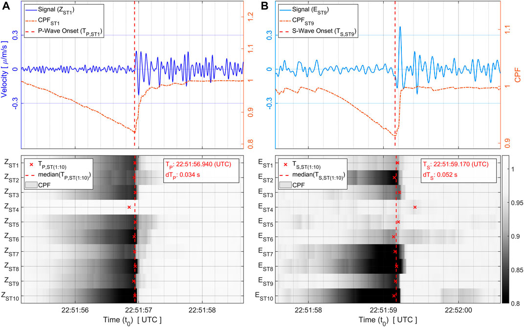
FIGURE 6. Determination of statistical changepoints for the P- and S-wave arrivals for the exemplary event from the Insheim reservoir (M_L 0.5, BAZ to network localization: 97.5°). (A) Top: Z component recorded at station ST1 (zero phase filter between 5 and 25 $Hz$) within the time interval $〈\mathit{argmax}\left(MC\right)-0.5s:\mathit{argmax}\left(MC\right)+3s〉$ and the corresponding evaluation of ${CPF}_{ST1}$. The minimum of ${CPF}_{ST1}$ gives an estimate of the P-wave arrival time at site ST1 ($T_{P,ST1}$). Bottom: Amplitude of $CPF$ over time for the Z components from all 10 array sites. The minima provide consistent estimates for the P-wave onsets ($T_{P,ST\left(1:10\right)}$). The low SNR at site ST4 distorts the minimum of ${CPF}_{ST4}$ (short period sensor). The median of $T_{P,ST\left(1:10\right)}$ is not influenced by the outlier. (B) Top: East component recorded at station ST9 (zero phase filter between 5 and 25 $Hz$) within the time interval $〈T_P+0.5s:T_P+3.5s〉$ and the corresponding evaluation of ${CPF}_{ST9}$. Bottom: Amplitude of $CPF$ over time for all East components. The minima provide estimates for the S-wave onsets ($T_{S,ST\left(1:10\right)}$).

Assuming a homogeneous velocity distribution, the epicentral distance $d$ is calculated using a P-wave velocity $v_P$ and a fixed $v_P/v_S$ ratio ($v_{P/S})$:

$d=\left(T_S-T_P\right)\left(\frac{v_P}{v_{\raisebox{1ex}{$P$}\!\left/ \!\raisebox{-1ex}{$S$}\right.}-1}\right)(23)$

Associated errors are derived using error propagation:

$\delta d=\sqrt{{\left(\frac{v_P}{v_{\raisebox{1ex}{$P$}\!\left/ \!\raisebox{-1ex}{$S$}\right.}-1}{\delta T}_P\right)}^2+{\left(\frac{v_P}{v_{\raisebox{1ex}{$P$}\!\left/ \!\raisebox{-1ex}{$S$}\right.}-1}{\delta T}_S\right)}^2+{\left(\frac{\left(T_S-T_P\right)}{v_{\raisebox{1ex}{$P$}\!\left/ \!\raisebox{-1ex}{$S$}\right.}-1}\delta v_P\right)}^2+{\left(\frac{\left(T_S-T_P\right)v_P}{{\left(v_{\raisebox{1ex}{$P$}\!\left/ \!\raisebox{-1ex}{$S$}\right.}-1\right)}^2}\delta v_{\raisebox{1ex}{$P$}\!\left/ \!\raisebox{-1ex}{$S$}\right.}\right)}^2}(24)$

The final localization of an event is defined by the distance $d$ and the back azimuth angle $\theta$, resulting from the array analysis (Eq. 13.1). It can be transformed to Cartesian coordinates, with $d_x=\mathrm{d}\sin \left(\theta \right)$ and $d_y=\mathrm{d}\cos \left(\theta \right)$. The corresponding errors are:

$\delta d_x=\sqrt{{\left(\sin \left(\theta \right)\delta d\right)}^2+{\left(\mathrm{d}\cos \left(\theta \right)\delta \theta \right)}^2}$(25.1)

$\delta d_y=\sqrt{{\left(\cos \left(\theta \right)\delta d\right)}^2+{\left(-\mathrm{d}\sin \left(\theta \right)\delta \theta \right)}^2}$(25.2)

Latitude and Longitude are calculated with reference to the geometrical mean of the array coordinates.

4 Results for the Insheim and Landau deep-geothermal reservoirs

We compare our results to a data catalogue of 77 induced seismic events from the Insheim and Landau deep-geothermal reservoirs. The catalogue was provided by the Geological Survey and Mining Authority of Rhineland-Palatinate (LGB-RLP, 2022). It covers a period from July 2021 to May 2022 and includes events in the magnitude range from M_L -0.2 to M_L 1.3. The events were detected using the Südpfalz network (LGB-RLP, 2022) and a template correlation detector (Vasterling et al., 2017). Localizations were performed using Seismic Handler (Stammler, 1993) and an optimized minimum 1-D velocity model (Küperkoch et al., 2018).

We re-localize all events using the seismic array in the Palatinate Forest and the methods introduced in section 3. The data from all 10 sites are taken in 20 s windows, starting 5 s ahead of the source times defined by the data catalogue. The waveforms are bandpass filtered between 5 and 25 $Hz$, and the instrument response is removed. Afterwards, the data are processed in 1.5 $s$ windows using the IRLS algorithm. They are continuously shifted by 10 samples (0.05 $s$), which results in a continuous function of the median cross correlation $MC$, the back azimuth θ, and the horizontal apparent velocity $v_{app,h}$ with time. Results for each event are obtained for the time window that minimizes the root mean squared error of the linear regression ($\mathit{argmin}\left(RMSE\left(\stackrel{\rightharpoonup }{\tau }\right)\right)$. Distance estimates are calculated using a constant $v_P/v_S$ ratio of 1.76 ± 0.03 and constant P-wave velocities ($v_P$) of 5.15 ± 0.2 $km/s$ and 5.25 ± 0.2 $km/s$ for events from the Landau and Insheim reservoirs, respectively. The values for $v_P$ were determined empirically, by minimizing the deviation from the network localizations. They are in very good agreement with a Granite layer (depth: >3 $km$, $v_P/v_S$: 1.76, $v_P$: 5.2 $km/s$) in the 1-D VSP velocity model for the Insheim reservoir (see Küperkoch et al., 2018). The homogeneous velocity models are optimized to localize events from the two reservoirs and are not adequate for differing source regions. The results from the array analysis and the corresponding localizations are summarized in Supplementary Tables S1, S2 in the supplements.

Figure 7A shows processing results for the exemplary event from the Insheim reservoir (19 November 2021; M_L 0.5). The solutions for back azimuth and horizontal apparent velocity are very consistent during the period of increased correlation, which is associated with the seismic phases traversing the array. The upper plot additionally shows $RMSE\left(\stackrel{\rightharpoonup }{\tau }\right)$ in dependence of the position of the analysis window. Figure 7B compares array and network localization. The distance between both methods is 0.8 $km$, which is well within the statistical errors.

FIGURE 7

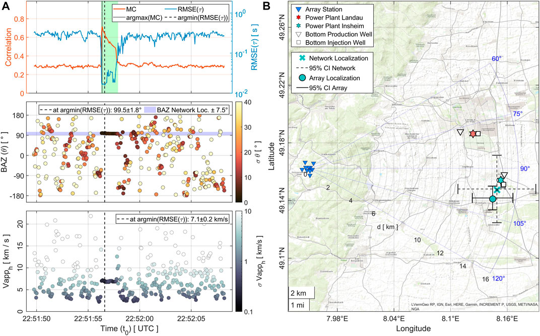
FIGURE 7. Results for the exemplary event in the Insheim Reservoir (M_L 0.5). (A) Top: Median of the cross-correlation matrix ($MC$, red line) and root mean squared error of the regression results (RMSE(τ), blue line) with time. The black dotted line indicates the point of maximum correlation ($\mathit{argmax}\left(MC\right)$). Results are taken for the solution that minimizes the error of the regression model ($\mathit{argmin}\left(RMSE\right)$, black dashed line). Center & Bottom: Time dependent back azimuth (BAZ) and horizontal apparent velocity ($v_{app,h}$). The solution for both parameters is consistent for the period of increased correlation (see green area in the plot above); before and after the results are random observations. This is also indicated by the standard errors (colors), which decrease with increasing correlation. (B) Map plot of the network (cross) and array localization (filled circle). The distance between both localizations is 0.8 $km$ and lies within the 95% confidence interval for both methods.

Figure 8 compares array and network localizations for the entire data catalogue (Figure 8A). Most array localizations form distinct clusters and can be clearly attributed to either the Insheim or the Landau reservoir (Figure 8B). However, there are some outliers that do not yield reliable results and are far from the network localizations (small map in Figure 8B). Figure 8C gives an overview of the statistics for the array and network localizations. Here, the BAZ and distance of the network localizations are given with reference to the position of the array. The distance estimates resulting from the array analysis are very consistent and usually within a few hundred meters from the network localization. The BAZ values, however, reveal a small and systematic misdirection of +4.1° for the Insheim and – 4.7° for the Landau events.

FIGURE 8

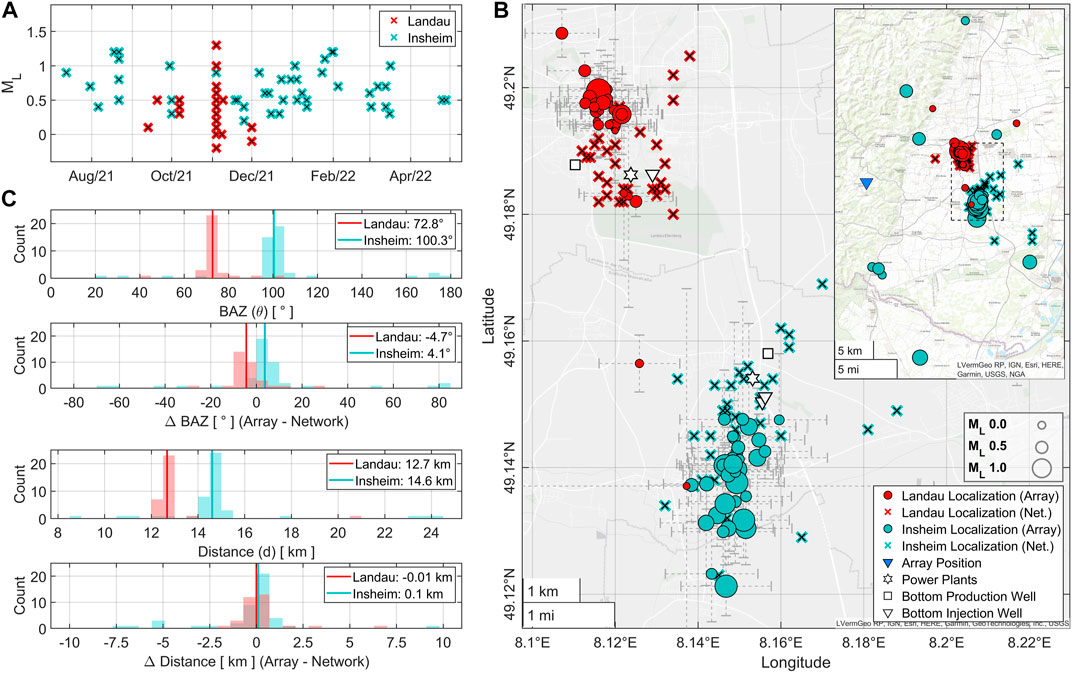
FIGURE 8. Comparison between array and network localizations for 77 induced events from the Insheim and Landau deep-geothermal reservoirs. (A) Local magnitudes (M_L) for events in the Insheim (cyan crosses) and Landau (red crosses) reservoirs in the period from July 2021 to May 2022 (data catalogue; LGB-RLP, 2022). (B) Map view of the array (circles) and network localizations (crosses) close to the power plants. The Landau and Insheim clusters are well separated. Error bars in the background represent the standard errors for the array localizations ($\delta d_x$ and $\delta d_y$). The upper right map shows the regional setting and reveals outlying localizations. (C) Histogram plots for BAZ (first plot) and distance (third plot) derived for the array localizations, separately for Insheim (cyan) and Landau (red). The median values are: Insheim: 100.3°, 14.6 $km$; Landau: 72.8°, 12.7 $km$. The second and fourth plot show the deviations between array and network approach. Here, in case of network results, BAZ and distance are calculated with reference to the position of the array. The distance estimates are very consistent (median deviation below 100 m). The back azimuth calculations, however, reveal a small and systematic misdirection of +4.1° for the Insheim and – 4.7° for the Landau events.

To investigate the quality of the array analysis, Figure 9A visualizes the array localizations, color-coded by the weighted root mean squared error of the regression analysis (cf. equations 10 and 18). The outlying localizations clearly correspond to low-quality linear regression models and involve large standard errors (${\sigma d}_x$ and ${\sigma d}_y$). This validates the error estimation. For a final comparison between network and array localizations, we correct the systematic misdirection of the back azimuth angle derived from the array analysis (Figure 9B). The resulting median distance between the two methods is 0.9 $km$, with a median absolute deviation ($MAD$) of 0.45 $km$.

FIGURE 9

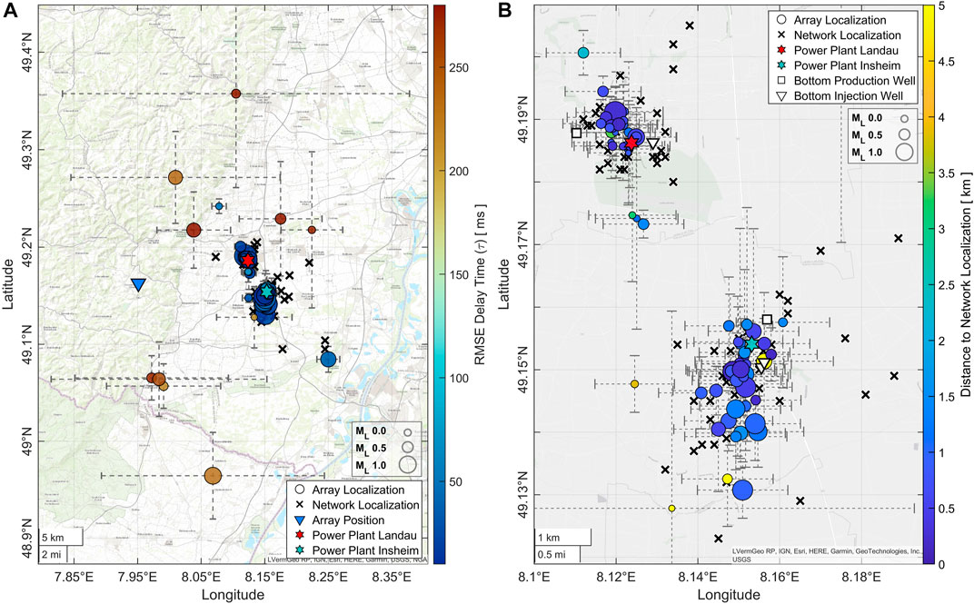
FIGURE 9. Performance of the array analysis. (A) Map view of the array (circles) and network localizations (black crosses). The array localizations are color coded by the $RMSE$ of the linear regression in the array analysis. The size of the circles scales with the magnitude (M_L). Outlying localizations are clearly associated with high $RMSE$ values and feature large standard errors (${\sigma d}_x$ and ${\sigma d}_y$). (B) Map view of the array (circles) and network (black crosses) localizations near the power plants. The array localizations are corrected for a systematic misdirection of the back azimuth in dependence of the origin (cf. Figure 8C). Array localizations are color coded by the distance to the corresponding network localizations. The median distance is 0.9 $km$, the median absolute deviation 0.45 $km$.

5 Discussion

Most of the array localizations show a remarkable agreement with the network localizations (median deviation <1 km) and especially the distance estimates are highly consistent. The BAZ calculations feature a systematic misdirection, which can be attributed to either an inadequate velocity model (i.e., 2-D/3-D effects) or local subsurface heterogeneities at the array. The assumption of a uniform velocity distribution is a simplification, and the velocity models are designed to localize seismicity from the two reservoirs. Therefore, the implementation of a more accurate velocity model could further improve the localization accuracy within the reservoirs.

Examining the outliers reveals a direct link between low-quality regression results (i.e., large $RMSE$) and low signal to noise conditions (Figure 10A). Most significant outliers occur during the period between December 2021 and February 2022, which might relate to an increased level of seismic noise in the northern hemisphere during winter times (see, e.g., Stutzmann et al., 2009). On the other hand, the corresponding network localizations are also located away from the main clusters of the reservoirs (Figure 10B), either indicating a reduced quality of the network localizations or a slightly different source region within the reservoir. The latter might involve differing source field characteristics, probably hampering an accurate signal recognition at the location of the array. This scenario is supported by a re-evaluation of a low-quality localization from 15 December 2021 (M_L 0.7), using an adapted bandpass filter between 25 and 35 $Hz$ (Supplementary Figure S3). The adjusted frequency band yields a more reliable regression result (though the errors remain large), which suggests wavefield characteristics that differ from a typical event from the reservoirs. In such a case, advanced methods in the spectral domain could yield improved results. Seydoux et al. (2016), for example, analyze the spatial coherence of the seismic wavefield by an eigenvalue decomposition of the covariance matrix. Incoherent noise is then minimized through a reduction of the signal to components related to the dominant eigenvalue. The PMCC algorithm (Cansi, 1995) calculates cross-correlation functions within narrow frequency bands, thus offering an improved separation between frequency bands with and without noise. On the downside, those methods are either computationally more expensive or require manual adjustments to the signal and noise characteristics.

FIGURE 10

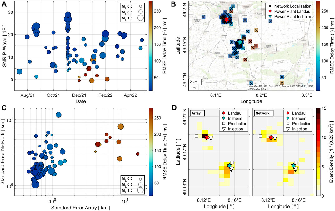
FIGURE 10. Origin of the outliers, statistical errors and distribution of the seismicity within the reservoirs. (A) Signal to noise ratio (SNR) of the P-Waves plotted against the time of occurrence and color coded by the $RMSE$ of the regression analysis. Low-quality results correspond to events with small SNR between December 2021 and February 2022. There is not a strong correlation between magnitude and low SNR during this period. (B) Network localizations (black crosses), highlighted by the $RMSE$ of the corresponding array analysis. It shows that outlying array localizations often agree with network localizations that are also farther from the center of the network clusters. (C) Standard errors for array and network localizations (mean of ${\sigma d}_x$ and ${\sigma d}_y$), color coded by the $RMSE$ of the linear regression from the array analysis. The statistical errors of the array approach are mostly smaller if compared to errors resulting for the network. (D) Event density, calculated in 0.25 ${km}^2$ units, for array (left) and network (right) localizations. The array localizations cluster more distinctly, especially in case of the Landau reservoir.

The statistical errors for the array and network localizations consistently increase with decreasing localization quality (Figure 10C). This is a good validation of the error calculation, which is crucial for the quality assessment during real-time processing. The standard errors associated with low-quality array localizations, derived in the winter of 2021/2022, are exceptionally large and coincide with large errors for the corresponding network localizations. It is important to note that the errors from the array analysis are generally smaller when compared to errors resulting for the network localizations. This might partly be due to the different calculation approaches, but more likely it reflects the superior location characteristics at the array. Here, the seismic noise level is in average 0.1 $\mu m/s$ (at 1–25 $Hz$), which is about 100 times smaller if compared to the Upper Rhine Graben (10 $\mu m/s$ at 1–40 $Hz$; Ritter & Sudhaus, 2007). Further, the network analysis and associated statistical errors are likely distorted by local 3-D velocity anomalies. For the array approach, the similarity of the ray paths between source and receivers involves smaller statistical errors (provided the data quality at the array sites is good). In this case, the expected errors have a systematic origin and relate to the uncertainty of the adapted uniform velocity model.

Figure 10D examines the distribution of the seismicity within the two reservoirs, separately for array and network localizations. It shows that the array results cluster more distinctly, especially for the Landau reservoir. Here, the events focus between injection and production well. The corresponding network localizations also mainly occur between injection and production side, but they scatter more widely. In the case of the Insheim reservoir, seismicity is concentrated southwest of the injection wells for both localization methods. Again, the horizontal variation is smaller for the array localizations. At this point it is difficult to conclude which results are more accurate. Looking at source-receiver distances exclusively, the 1-D velocity model used in the network analysis is not superior to an optimized uniform model. However, the missing depth dependence in the array approach also affects the epicentral localization.

Our regression approach includes inter-station elevation differences, which allows for estimates of the full 3-D slowness vector. In Figure 11 we investigate results for the horizontal and vertical apparent velocities ($v_{app,h}$ and $v_{app,z}$), and the vertical angle of incidence $i=\mathit{atan}\left(v_{app,z}/v_{app,h}\right)$, for the entire data catalogue. The horizontal apparent velocity is mostly between 6 and 8 $km/s$ (median: 6.6 $km/s$, MAD: 0.4 $km/s$) and the vertical apparent velocity between 3 and 7 $km/s$ (median: 4.1 $km/s$, MAD: 1 $km/s$). The angles of incidence mostly range between 20° and 40°. For the Insheim reservoir, some events feature increased vertical apparent velocity values. The associated angles of incidence are larger than 50°. Low-quality regression results for the period between December 2021 and February 2022 involve very small values for the vertical apparent velocity and the vertical angle of incidence. Consistent with the results for the exemplary event (Section 3.2), errors associated with $v_{app,z}$ are distinctly larger if compared to the horizontal components. To estimate the vertical slowness component with sufficient accuracy, differences in elevation should be of the same order of magnitude as the horizontal distances between the array sites. In this case, the vertical angle of incidence could be used for depth estimation, e.g., using a vertical (borehole) array in combination with a conventional horizontal layout.

FIGURE 11

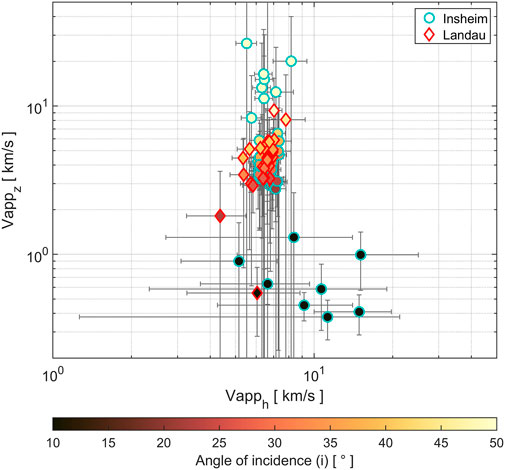
FIGURE 11. Horizontal and vertical apparent velocity and vertical angle of incidence for 77 induced events from the Insheim and Landau deep-geothermal reservoirs. Red and cyan marker edgings indicate results for the Landau and Insheim reservoirs, respectively. The color of the markers shows the corresponding angle of incidence $i=\mathit{atan}\left(v_{app,z}/v_{app,h}\right)$. Errors associated with the vertical apparent velocity ($v_{app,z}$) are distinctly larger if compared to the horizontal component ($v_{app,h}$). However, the estimated angles of incidence are mostly consistent and range between 20° and 40°. For the Insheim reservoir, some events feature increased vertical apparent velocity values; the associated angles of incidence are larger than 50°. Low-quality regression results from the period between December 2021 and February 2022 involve very small values for the vertical apparent velocity and the vertical angle of incidence.

Our analysis shows that conventional array processing techniques, such as f-k analysis or OLS regression, are highly sensitive to outlying data points and can heavily rely on manual adjustments of the evaluation parameters (window size and position, frequency band). Here, the IRLS algorithm, in combination with the Biweight function, must be preferred. It yields stable and consistent results, even in the presence of corrupted data. In comparison to a regular f-k analysis, it is less sensitive to the frequency band (but requires SNR >1 for the P wave onset) and is computationally more efficient. The application of the algorithm to real-time data involves a continuous evaluation of the cross-correlation function and continuous robust estimations of the slowness vector and associated uncertainties. If the correlation function exceeds a certain threshold, distance estimates are calculated. In case of insufficient processing results, indicated by the statistical errors, the event can be re-evaluated using an adapted frequency band. Here, an automatized choice of the filter settings can be based on the cross-spectral matrix of the signals. The computational efficiency of the algorithm would also allow for a second evaluation stream (i.e., secondary continuous calculations of the cross-correlation, the slowness vector and associated uncertainties) within a different frequency band.

6 Conclusion

We investigate the suitability of seismic arrays for monitoring multiple geothermal reservoirs from one central remote location. Here, the increased distance to the source requires accurate processing techniques to receive reliable earthquake localizations. We therefore employ robust linear regression to estimate the slowness vector of seismic phases and use statistical changepoint analysis to obtain automatized P- and S-wave arrival times, which can be used for distance calculations. The comparison to standard array processing tools, such as ordinary least-squares regression and f-k analysis, demonstrates that a robust approach is crucial to achieve localization accuracy suitable for geothermal monitoring. We further validate our results using a data catalogue of 77 network localizations for the Landau and Insheim deep-geothermal reservoirs, located in the Upper Rhine Graben. It shows that we can clearly separate earthquakes originating from the two reservoirs and the quality of the array localizations is at least comparable to those from the seismic network. Moreover, the remote location of the array involves a significantly lower level of seismic noise compared to the seismic network. This enhances the sensitivity to small magnitude events and ensures surveillance during noisy episodes.

Estimating the slowness vector of a seismic phase using linear regression relies on observed delay times, derived from inter-station cross-correlation functions. Here, we recommend using the median of the cross-correlation matrix as a robust trigger function as it remains unaffected by correlated noise between single station pairs or degraded signal to noise conditions at specific array sites.

We further demonstrate that incorporating elevation differences into the regression model allows for an estimation of the vertical slowness component ($s_z$). This separates the method from those limited to the horizontal plane, but the statistical significance and accuracy of the results must be evaluated with caution. If an array is to be used to accurately estimate the vertical apparent velocity (and subsequently the vertical angle of incidence), the elevation differences between the array sites should be of the same order of magnitude as the horizontal inter-station distances. However, elevation differences should be included in the array analysis if they are expected to contribute to the observed delay times. This eliminates the need for elevation correction terms, and the impact on the calculation time is only marginal.

When a set of observed delay times includes outliers, the use of robust array processing techniques is crucial. We therefore implement and test robust regression estimators for seismic array data. Here, iteratively reweighted least squares in combination with a Biweight function yields reliable parameter estimates, that are significantly more stable compared to conventional least squares regression and f-k analysis. The algorithm is computationally efficient, making it well suited for real-time applications.

To obtain P- and S-wave arrivals by an automated approach, we introduce statistical changepoint analysis as an alternative to autoregressive prediction. The determination of a statistical changepoint only relies on the calculation of a basic statistical parameter and not on autoregressive filtering. This makes it computationally more efficient, at least when the search problem is restricted to a single changepoint. The quality of the estimated arrival times is remarkable, resulting in highly accurate distance estimates for the array localizations.

The final comparison between network and array localizations shows that the results are very consistent. Most array localizations form distinct clusters that can be clearly attributed to either the Insheim or the Landau reservoir. A few outliers for the array localizations in the period between December 2021 and February 2022, coincide with low-quality network localizations in the outer reservoir domains. Upon closer examination of the seismicity within the two reservoirs, it becomes evident that the array results cluster more distinctly than the network results. Furthermore, the statistical errors from the array analysis are generally smaller compared to those from the network localizations. This reflects the superior location characteristics at the array, where the average seismic noise level is about 100 times lower than in the Upper Rhine Graben. As a result, the quality of the epicentral array localizations is at least comparable with those derived from the network.

Data availability statement

The raw data supporting the conclusions of this article will be made available by the authors, without undue reservation.

Author contributions

PH was responsible for the planning and setup of the seismic array. He developed the methodology and the software used to obtain the results and wrote the initial draft of the manuscript. ML was involved in the planning and realisation of the project. He participated in the determination of the array layout and setup and contributed to the final draft of the manuscript. GR conceived and initiated the project, taking responsibility for its execution. All authors contributed to the article and approved the submitted version.

Funding

This work was funded through the Federal Ministry for Economic Affairs and Climate Action of the Federal Republic of Germany as part of the SEIGER (Seismic monitoring of deep geothermal power plants and possible seismic impact) research project (FKZ 03EE4003F).

Acknowledgments

We thank the Geological Survey and Mining Authority of Rhineland-Palatinate (LGB-RLP), and particularly Bernd Schmidt and Helmuth Winter, for their support during the setup of the array and for providing the earthquake catalogue. We thank KH, FN, VT, LDS for their careful and constructive comments, which improved the manuscript.

Conflict of interest

The authors declare that the research was conducted in the absence of any commercial or financial relationships that could be construed as a potential conflict of interest.

Publisher’s note

All claims expressed in this article are solely those of the authors and do not necessarily represent those of their affiliated organizations, or those of the publisher, the editors and the reviewers. Any product that may be evaluated in this article, or claim that may be made by its manufacturer, is not guaranteed or endorsed by the publisher.

Supplementary material

The Supplementary Material for this article can be found online at: https://www.frontiersin.org/articles/10.3389/feart.2023.1217587/full#supplementary-material

References

Akaike, H. (1973). Maximum likelihood identification of Gaussian autoregressive moving average models. Biometrika 60 (2), 255–265. doi:10.1093/biomet/60.2.255

CrossRef Full Text | Google Scholar

Auger, I. E., and Lawrence, C. E. (1989). Algorithms for the optimal identification of segment neighborhoods. Bull. Math. Biol. 51 (1), 39–54. doi:10.1016/S0092-8240(89)80047-3

PubMed Abstract | CrossRef Full Text | Google Scholar

Bartz, J. (1974). “Die Mächtigkeit des Quartärs im Oberrheingraben,” in Approaches to taphrogenesis. Editors J. H. Illies, and K. Fuchs (Stuttgart, Germany: Schweitzerbarth), 78–87.

Google Scholar

Beaton, A. E., and Tukey, J. W. (1974). The fitting of power series, meaning polynomials, illustrated on band-spectroscopic data. Technometrics 16 (2), 147–185. doi:10.1080/00401706.1974.10489171

CrossRef Full Text | Google Scholar

BGR, (2023). Bundesanstalt für Geowissenschaften und Rohstoffe. https://www.bgr.bund.de/DE/Themen/Erdbeben-Gefaehrdungsanalysen/Seismologie/Seismologie/GERSEIS/gerseis_node.html (Accessed June 02, 2023).

Google Scholar

Bishop, J. W., Fee, D., and Szuberla, C. A. (2020). Improved infrasound array processing with robust estimators. Geophys. J. Int. 221 (3), 2058–2074. doi:10.1093/gji/ggaa110

CrossRef Full Text | Google Scholar

Brune, J., and Thatcher, W. (2002). “Strength and energetics of active fault zones,” International handbook of earthquake and engineering seismology, Part A. Editors W. H. K. Lee, H. Kanamori, C. J. Paul, and H. Kisslinger (Int. Assoc. Seismol. Phys. Earth's Interior, Comm. Educ), 81, 569–588.

CrossRef Full Text | Google Scholar

Cansi, Y. (1995). An automatic seismic event processing for detection and location: The PMCC method. Geophys. Res. Lett. 22 (9), 1021–1024. doi:10.1029/95GL00468

CrossRef Full Text | Google Scholar

Capon, J. (1969). High-resolution frequency-wavenumber spectrum analysis. Proc. IEEE 57 (8), 1408–1418. doi:10.1109/PROC.1969.7278

CrossRef Full Text | Google Scholar

Chen, J., and Gupta, A. K. (1997). Testing and locating variance changepoints with application to stock prices. J. Am. Stat. Assoc. 92 (438), 739–747. doi:10.1080/01621459.1997.10474026

CrossRef Full Text | Google Scholar

Chen, J., and Gupta, A. K. (2001). On change point detection and estimation. Commun. statistics-simulation Comput. 30 (3), 665–697. doi:10.1081/SAC-100105085

CrossRef Full Text | Google Scholar

Claerbout, J. F. (1986). Fundamentals of geophysical data processing, 2nd edn. J. R. Astron. Soc. 86, 217–219. doi:10.1111/j.1365-246X.1986.tb01085.x86

CrossRef Full Text | Google Scholar

Coombs, M. L., Wech, A. G., Haney, M. M., Lyons, J. J., Schneider, D. J., Schwaiger, H. F., et al. (2018). Short-term forecasting and detection of explosions during the 2016–2017 eruption of Bogoslof volcano, Alaska. Front. Earth Sci. 6, 122. doi:10.3389/feart.2018.00122

CrossRef Full Text | Google Scholar

Cornet, F. H., Helm, J., Poitrenaud, H., and Etchecopar, A. (1997). Seismic and aseismic slips induced by large-scale fluid injections. Pure Appl. Geophys. 150, 563–583. doi:10.1007/978-3-0348-8814-1_12

CrossRef Full Text | Google Scholar

Cornet, F. H., and Jianmin, Y. (1995). Analysis of induced seismicity for stress field determination and pore pressure mapping. PAGEOPH 145, 677–700. doi:10.1007/BF00879595

CrossRef Full Text | Google Scholar

Cornet, F. H., and Julien, Ph. (1989). Stress determination from hydraulic test data and focal mechanisms of induced seismicity. Int. J. Rock Mech. Min. Sci. Geomechanics Abstr. 26 (3-4), 235–248. doi:10.1016/0148-9062(89)91973-6

CrossRef Full Text | Google Scholar

Cuenot, N., Dorbath, C., and Dorbath, L. (2008). Analysis of the microseismicity induced by fluid injections at the EGS site of soul-sous-forêts (alae, France): Implications for the characterization of the geothermal reservoir properties. Pure Appl. Geophys. 165, 797–828. doi:10.1007/s00024-008-0335-7

CrossRef Full Text | Google Scholar

De Angelis, S., Haney, M. M., Lyons, J. J., Wech, A., Fee, D., Diaz-Moreno, A., et al. (2020). Uncertainty in detection of volcanic activity using infrasound arrays: Examples from Mt. Etna, Italy. Front. Earth Sci. 8, 169. doi:10.3389/feart.2020.00169

CrossRef Full Text | Google Scholar

Del Pezzo, E., and Giudicepietro, F. (2002). Plane wave fitting method for a plane, small aperture, short period seismic array: A MATHCAD program. Comput. geosciences 28 (1), 59–64. doi:10.1016/S0098-3004(01)00076-0

CrossRef Full Text | Google Scholar

Doebl, F., and Olbrecht, W. (1974). “An isobath map of the Tertiary base in the Rhinegraben,” in Approaches to taphrogenesis. Editors J. H. Illies, and K. Fuchs (Stuttgart, Germany: Schweitzerbarth), 71–72.

Google Scholar

Dornstadter, J., Kappelmeyer, O., and Welter, M. (1999). “The geothermal potential in the Upper Rhine Graben valley,” in Proceedings of the European Geothermal Conference Basel '99 (Basel, Switzerland) 2, 77–85.

Google Scholar

Douglas, A., Bowers, D., Marshall, P. D., Young, J. B., Porter, D., and Wallis, N. J. (1999). Putting nuclear-test monitoring to the test. Nature 398 (6727), 474–475. doi:10.1038/19000

CrossRef Full Text | Google Scholar

Dumouchel, W., and O’brien, F. (1989). “Integrating a robust option into a multiple regression computing environment,” in Computer science and statistics: Proceedings of the 21st symposium on the interface (Alexandria, Egypt: American Statistical Association), 297–302.

Google Scholar

Evans, K. F., Zappone, A., Kraft, T., Deichmann, N., and Moia, F. (2012). A survey of the induced seismic responses to fluid injection in geothermal and CO2 reservoirs in Europe. Geothermics 41, 30–54. doi:10.1016/j.geothermics.2011.08.002

CrossRef Full Text | Google Scholar

Farahbod, A. M., Kao, H., Cassidy, J. F., and Walker, D. (2015). How did hydraulic-fracturing operations in the Horn River Basin change seismicity patterns in northeastern British Columbia, Canada? Lead. Edge 34 (6), 658–663. doi:10.1190/tle34060658.1,

CrossRef Full Text | Google Scholar

Gibbons, S. J., Kværna, T., and Ringdal, F. (2010). Considerations in phase estimation and event location using small-aperture regional seismic arrays. Pure Appl. Geophys. 167, 381–399. doi:10.1007/s00024-009-0024-1

CrossRef Full Text | Google Scholar

Gibbons, S. J., Kværna, T., and Ringdal, F. (2005). Monitoring of seismic events from a specific source region using a single regional array: A case study. J. Seismol. 9, 277–294. doi:10.1007/s10950-005-5746-7

CrossRef Full Text | Google Scholar

Gibbons, S. J., Näsholm, S. P., Ruigrok, E., and Kværna, T. (2018). Improving slowness estimate stability and visualization using limited sensor pair correlation on seismic arrays. Geophys. J. Int. 213 (1), 447–460. doi:10.1093/gji/ggx550

CrossRef Full Text | Google Scholar

Gibbons, S. J., Ringdal, F., and Kværna, T. (2008). Detection and characterization of seismic phases using continuous spectral estimation on incoherent and partially coherent arrays. Geophys. J. Int. 172 (1), 405–421. doi:10.1111/j.1365-246X.2007.03650.x

CrossRef Full Text | Google Scholar

Groos, J. C., and Ritter, J. R. (2014). Verbundprojekt MAGS - konzepte zur Begrenzung der mikroseismischen Aktivität bei der energetischen Nutzung geothermischer Systeme im tiefen Untergrund, Einzelprojekt 1: Quantifizierung und Charakterisierung des induzierten seismischen Volumens im Bereich Landau/Südpfalz. Germany: Karlsruher Institut für Technologie, Final Report of the Project MAGS.

Google Scholar

Grubbs, F. E. (1969). Procedures for detecting outlying observations in samples. Technometrics 11 (1), 1–21. doi:10.1080/00401706.1969.10490657

CrossRef Full Text | Google Scholar

Grünthal, G. (2014). Induced seismicity related to geothermal projects versus natural tectonic earthquakes and other types of induced seismic events in Central Europe. Geothermics 52, 22–35. doi:10.1016/j.geothermics.2013.09.009

CrossRef Full Text | Google Scholar

Grünthal, G., and Wahlström, R. (2012). The European-Mediterranean earthquake catalogue (EMEC) for the last millennium. J. Seismol. 16, 535–570. doi:10.1007/s10950-012-9302-y

CrossRef Full Text | Google Scholar

Haneke, J., and Weidenfeller, M. (2010). “Die geologischen baueinheiten der Pfalz,” in Geographie der Pfalz (Landau/Pfalz, Germany: Pfälzische Landeskunde).

Google Scholar

Haney, M. M., Van Eaton, A. R., Lyons, J. J., Kramer, R. L., Fee, D., and Iezzi, A. M. (2018). Volcanic thunder from explosive eruptions at Bogoslof volcano, Alaska. Geophys. Res. Lett. 45 (8), 3429–3435. doi:10.1002/2017GL076911

CrossRef Full Text | Google Scholar

Holland, P. W., and Welsch, R. E. (1977). Robust regression using iteratively reweighted least-squares. Commun. Statistics-theory Methods 6 (9), 813–827. doi:10.1080/03610927708827533

CrossRef Full Text | Google Scholar

Huber, P. J. (1973). Robust regression: Asymptotics conjectures and Monte Carlo. Ann. Statistics 1 (5), 799–821. doi:10.1214/aos/1176342503

CrossRef Full Text | Google Scholar

Huber, P. J. (1981). Robust statistics. New York, NY, USA: John Wiley and Sons, Inc.

Google Scholar

Hurtig, E., Cermak, V., Haenel, R., and Zui, V. (1992). Geothermal atlas of Europe. Vienna, Austria: International Atomic Energy Agency.

Google Scholar

Illies, J. H. (1972). The Rhine graben rift system-plate tectonics and transform faulting. Geophys. Surv. 1 (1), 27–60. doi:10.1007/BF01449550

CrossRef Full Text | Google Scholar

Jackson, B., Scargle, J. D., Barnes, D., Arabhi, S., Alt, A., Gioumousis, P., et al. (2005). An algorithm for optimal partitioning of data on an interval. IEEE Signal Process. Lett. 12 (2), 105–108. doi:10.1109/LSP.2001.838216

CrossRef Full Text | Google Scholar

Johnson, S. W., Chambers, D. J., Boltz, M. S., and Koper, K. D. (2021). Application of a convolutional neural network for seismic phase picking of mining-induced seismicity. Geophys. J. Int. 224 (1), 230–240. doi:10.1093/gji/ggaa449

PubMed Abstract | CrossRef Full Text | Google Scholar

Joswig, M. (1990). Pattern recognition for earthquake detection. Bull. Seismol. Soc. Am. 80 (1), 170–186. doi:10.1785/BSSA0800010170

CrossRef Full Text | Google Scholar

Killick, R., Fearnhead, P., and Eckley, I. A. (2012). Optimal detection of changepoints with a linear computational cost. J. Am. Stat. Assoc. 107 (500), 1590–1598. doi:10.1080/01621459.2012.737745

CrossRef Full Text | Google Scholar

King, D. W., Haddon, R. A. W., and Husebye, E. S. (1975). Precursors to PP. Phys. Earth Planet. Interiors 10 (2), 103–127. doi:10.1016/0031-9201(75)90029-1

CrossRef Full Text | Google Scholar

King, D. W., Husebye, E. S., and Haddon, R. A. W. (1976). Processing of seismic precursor data. Phys. Earth Planet. Interiors 12 (2-3), 128–134. doi:10.1016/0031-9201(76)90042-X

CrossRef Full Text | Google Scholar

Krüger, F., Dahm, T., and Hannemann, K. (2020). Mapping of Eastern North Atlantic Ocean seismicity from Po/So observations at a mid-aperture seismological broad-band deep sea array. Geophys. J. Int. 221 (2), 1055–1080. doi:10.1093/gji/ggaa054

CrossRef Full Text | Google Scholar

Küperkoch, L., Meier, T., Brüstle, A., Lee, J., and Friederich, W. (2012). Automated determination of S-phase arrival times using autoregressive prediction: Application to local and regional distances. Geophys. J. Int. 188 (2), 687–702. doi:10.1111/j.1365-246X.2011.05292.x

CrossRef Full Text | Google Scholar

Küperkoch, L., Meier, T., Lee, J., Friederich, W., and Egelados Working Group, (2010). Automated determination of P-phase arrival times at regional and local distances using higher order statistics. Geophys. J. Int. 181 (2), 1159–1170. doi:10.1111/j.1365-246X.2010.04570.x

CrossRef Full Text | Google Scholar

Küperkoch, L., Olbert, K., and Meier, T. (2018). Long-term monitoring of induced seismicity at the Insheim geothermal site, Germany. Bull. Seismol. Soc. Am. 108 (6), 3668–3683. doi:10.1785/0120170365

CrossRef Full Text | Google Scholar

Kværna, T., and Doornbos, D. J. (1991). Scattering of regionalP n by moho topography. Geophys. Res. Lett. 18 (7), 1273–1276. doi:10.1029/91GL01292

CrossRef Full Text | Google Scholar

Kværna, T., and Ringdal, F. (1986). NORSAR scientific rep 1-86/87. Stab. Var. fk Estim. Tech., 29–40.

Google Scholar

Lai, T. L., Robbins, H., and Wei, C. Z. (1978). Strong consistency of least squares estimates in multiple regression. PNAS 75 (7), 3034–3036. doi:10.1073/pnas.75.7.3034

PubMed Abstract | CrossRef Full Text | Google Scholar

Leonard, M., and Kennett, B. L. N. (1999). Multi-component autoregressive techniques for the analysis of seismograms. Phys. Earth Planet. Interiors 113 (1-4), 247–263. doi:10.1016/S0031-9201(99)00054-0

CrossRef Full Text | Google Scholar

Leva, C., Rümpker, G., and Wölbern, I. (2022). Multi-array analysis of volcano-seismic signals at Fogo and Brava, Cape Verde. Solid earth. 13, 1243–1258. doi:10.5194/se-13-1243-2022

CrossRef Full Text | Google Scholar

Leva, C., Rümpker, G., and Wölbern, I. (2020). Remote monitoring of seismic swarms and the August 2016 seismic crisis of Brava, Cabo Verde, using array methods. Nat. Hazards Earth Syst. Sci. 20 (12), 3627–3638. doi:10.5194/nhess-20-3627-2020

CrossRef Full Text | Google Scholar

LGB-RLP, (2022). Landesamt für Geologie und Bergbau Rheinland-Pfalz. https://www.lgb-rlp.de/de/fachthemen/landeserdbebendienstrlp/forschungsprojekt-seiger.html (Accessed February 08, 2023).

Google Scholar

Li, W., Chakraborty, M., Fenner, D., Faber, J., Zhou, K., Rümpker, G., et al. (2022). EPick: Attention-based multi-scale UNet for earthquake detection and seismic phase picking. Front. Earth Sci. 10. doi:10.3389/feart.2022.953007

CrossRef Full Text | Google Scholar

Li, Z., and Zhan, Z. (2018). Pushing the limit of earthquake detection with distributed acoustic sensing and template matching: A case study at the Brady geothermal field. Geophys. J. Int. 215 (3), 1583–1593. doi:10.1093/gji/ggy359

CrossRef Full Text | Google Scholar

Lomax, A., Virieux, J., Volant, P., and Berge-Thierry, C. (2000). “Probabilistic earthquake location in 3D and layered models,” in Advances in seismic event location. Modern approaches in geophysics. Editors C. Thurber, and N. Rabinowitz (Dordrecht, Netherlands: Springer), 101–134. doi:10.1007/978-94-015-9536-0_5

CrossRef Full Text | Google Scholar

Majer, E. L., Baria, R., Stark, M., Oates, S., Bommer, J., Smith, B., et al. (2007). Induced seismicity associated with enhanced geothermal systems. Geothermics 36 (3), 185–222. doi:10.1016/j.geothermics.2007.03.003

CrossRef Full Text | Google Scholar

Mousavi, S. M., Ellsworth, W. L., Zhu, W., Chuang, L. Y., and Beroza, G. C. (2020). Earthquake transformer—An attentive deep-learning model for simultaneous earthquake detection and phase picking. Nat. Commun. 11, 3952. doi:10.1038/s41467-020-17591-w

PubMed Abstract | CrossRef Full Text | Google Scholar

Olson, J. V., and Szuberla, C. A. (2005). Distribution of wave packet sizes in microbarom wave trains observed in Alaska. J. Acoust. Soc. Am. 117 (3), 1032–1037. doi:10.1121/1.1854651

CrossRef Full Text | Google Scholar

Picard, D. (1985). Testing and estimating change-points in time series. Adv. Appl. Probab. 17 (4), 841–867. doi:10.2307/1427090

CrossRef Full Text | Google Scholar

Plenkers, K., Ritter, J. R. R., and Schindler, M. (2013). Low signal-to-noise event detection based on waveform stacking and cross-correlation: Application to a stimulation experiment. J. Seismol. 17, 27–49. doi:10.1007/s10950-012-9284-9

CrossRef Full Text | Google Scholar

Ritter, J. R., and Sudhaus, H. (2007). Characterization of small local noise sources with array seismology. Near Surf. Geophys. 5 (4), 253–261. doi:10.3997/1873-0604.2007007

CrossRef Full Text | Google Scholar

Rost, S., and Thomas, C. (2002). Array seismology: Methods and applications. Rev. Geophys. 40 (3), 2–27. doi:10.1029/2000RG000100

CrossRef Full Text | Google Scholar

Rousseeuw, P. J. (1984). Least median of squares regression. J. Am. Stat. Assoc. 79 (388), 871–880. doi:10.1080/01621459.1984.10477105

CrossRef Full Text | Google Scholar

Rousseeuw, P. J., and Leroy, A. M. (1987). Robust regression and outlier detection. Hoboken, New Jersey, United States: John Wiley and Sons, Inc.

Google Scholar

Schweitzer, J., Fyen, J., Mykkeltveit, S., Gibbons, S. J., Pirli, M., Kühn, D., et al. (2012). Seismic arrays. New Man. Seismol. observatory Pract. 2 (NMSOP-2), 1–80. doi:10.2312/GFZ.NMSOP-2_ch9

CrossRef Full Text | Google Scholar

Sen, A., and Srivastava, M. S. (1975). On tests for detecting change in mean. Ann. Statistics 3, 98–108. doi:10.1214/aos/1176343001

CrossRef Full Text | Google Scholar

Seydoux, L., Shapiro, N. M., De Rosny, J., and Landès, M. (2016). Spatial coherence of the seismic wavefield continuously recorded by the USArray. Geophys. Res. Lett. 43 (18), 9644–9652. doi:10.1002/2016GL070320

CrossRef Full Text | Google Scholar

Shi, X., Gallagher, C., Lund, R., and Killick, R. (2022). A comparison of single and multiple changepoint techniques for time series data. Comput. Statistics Data Analysis 170, 107433. doi:10.1016/j.csda.2022.107433

CrossRef Full Text | Google Scholar

Sick, B., Guggenmos, M., and Joswig, M. (2015). Chances and limits of single-station seismic event clustering by unsupervised pattern recognition. Geophys. J. Int. 201 (3), 1801–1813. doi:10.1093/gji/ggv126

CrossRef Full Text | Google Scholar

Singh, M., and Rümpker, G. (2020). Seismic gaps and intraplate seismicity around Rodrigues Ridge (Indian Ocean) from time domain array analysis. Solid earth. 11 (6), 2557–2568. doi:10.5194/se-11-2557-2020

CrossRef Full Text | Google Scholar

Sleeman, R., and Van Eck, T. (1999). Robust automatic P-phase picking: An on-line implementation in the analysis of broadband seismogram recordings. Phys. earth Planet. interiors 113 (1-4), 265–275. doi:10.1016/S0031-9201(99)00007-2

CrossRef Full Text | Google Scholar

Smith, P. J., and Bean, C. J. (2020). Retreat: A REal-time TREmor analysis tool for seismic arrays, with applications for volcano monitoring. Front. Earth Sci. 8, 586955. doi:10.3389/feart.2020.586955

CrossRef Full Text | Google Scholar

Stammler, K. (1993). SeismicHandler—Programmable multichannel data handler for interactive and automatic processing of seismological analyses. Comput. geosciences 19 (2), 135–140. doi:10.1016/0098-3004(93)90110-Q

CrossRef Full Text | Google Scholar

Steinberg, A., and Gaebler, P. (2023). Automatisch erstellter Erdbeben Katalog des Seiger Projektes. Zenodo. doi:10.5281/zenodo.7973593

CrossRef Full Text | Google Scholar

Stutzmann, E., Schimmel, M., Patau, G., and Maggi, A. (2009). Global climate imprint on seismic noise. Geochem. Geophys. Geosystems 10 (11). doi:10.1029/2009GC002619

CrossRef Full Text | Google Scholar

Suckale, J. (2010). Moderate-to-large seismicity induced by hydrocarbon production. Lead. Edge 29 (3), 310–319. doi:10.1190/1.3353728

CrossRef Full Text | Google Scholar

Szuberla, C. A., and Olson, J. V. (2004). Uncertainties associated with parameter estimation in atmospheric infrasound arrays. J. Acoust. Soc. Am. 115 (1), 253–258. doi:10.1121/1.1635407

PubMed Abstract | CrossRef Full Text | Google Scholar

Takanami, T., and Kitagawa, G. (1988). A new efficient procedure for the estimation of onset times of seismic waves. J. Phys. Earth 36 (6), 267–290. doi:10.4294/jpe1952.36.267

CrossRef Full Text | Google Scholar

VanDecar, J. C., and Crosson, R. S. (1990). Determination of teleseismic relative phase arrival times using multi-channel cross-correlation and least squares. Bull. Seismol. Soc. Am. 80 (1), 150–169. doi:10.1785/BSSA0800010150

CrossRef Full Text | Google Scholar

Vasterling, M., Wegler, U., Becker, J., Brüstle, A., and Bischoff, M. (2017). Real-time envelope cross-correlation detector: Application to induced seismicity in the Insheim and Landau deep geothermal reservoirs. J. Seismol. 21, 193–208. doi:10.1007/s10950-016-9597-1

CrossRef Full Text | Google Scholar

Velleman, P., and Welsch, R. (1981). Efficient computing of regression diagnostics. Effic. Comput. Regres. Diagnostics. Am. Statistician 35 (4), 234–242. doi:10.2307/2683296

CrossRef Full Text | Google Scholar

Wald, A. (1943). Tests of statistical hypotheses concerning several parameters when the number of observations is large. Trans. Am. Math. Soc. 54 (3), 426–482. doi:10.1090/s0002-9947-1943-0012401-3

CrossRef Full Text | Google Scholar

Wang, R., Schmandt, B., Zhang, M., Glasgow, M., Kiser, E., Rysanek, S., et al. (2020). Injection-induced earthquakes on complex fault zones of the Raton Basin illuminated by machine-learning phase picker and dense nodal array. Geophys. Res. Lett. 47 (14). doi:10.1029/2020GL088168

CrossRef Full Text | Google Scholar

Weingarten, M., Ge, S., Godt, J. W., Bekins, B. A., and Rubinstein, J. L. (2015). High-rate injection is associated with the increase in US mid-continent seismicity. Science 348, 1336–1340. doi:10.1126/science.aab1345

PubMed Abstract | CrossRef Full Text | Google Scholar

Wilson, D., Leon, J., Aster, R., Ni, J., Schlue, J., Grand, S., et al. (2002). Broadband seismic background noise at temporary seismic stations observed on a regional scale in the southwestern United States. Bull. Seismol. Soc. Am. 92 (8), 3335–3342. doi:10.1785/0120010234

CrossRef Full Text | Google Scholar

Withers, M., Aster, R., Young, C., Beiriger, J., Harris, M., Moore, S., et al. (1998). A comparison of select trigger algorithms for automated global seismic phase and event detection. Bull. Seismol. Soc. Am. 88 (1), 95–106. doi:10.1785/BSSA0880010095

CrossRef Full Text | Google Scholar

Yao, Y. C. (1988). Estimating the number of change-points via Schwarz'criterion. Statistics Probab. Lett. 6 (3), 181–189. doi:10.1016/0167-7152(88)90118-6

CrossRef Full Text | Google Scholar

Zang, A., Oye, V., Jousset, P., Deichmann, N., Gritto, R., McGarr, A., et al. (2014). Analysis of induced seismicity in geothermal reservoirs – an overview. Geothermics 52, 6–21. doi:10.1016/j.geothermics.2014.06.005

CrossRef Full Text | Google Scholar

Zhu, W., and Beroza, G. C. (2019). PhaseNet: A deep-neural-network-based seismic arrival-time picking method. Geophys. J. Int. 216 (1), 261–273. doi:10.1093/gji/ggy423

CrossRef Full Text | Google Scholar