Deep ensemble model-based moving object detection and classification using SAR images

1 Introduction

A device that is frequently utilized for a variety of remote sensing applications is the synthetic aperture radar (SAR). The SAR research community has significantly emphasized on the issue of automatic target recognition (ATR) among the other issues. It is well-known that optical and SAR pictures greatly differ [6]. Essentially, there are two key issues. The first is the presence of speckle noise brought on by a coherent backscattered signal collection. The second is the way that man-made things’ reflectivity changes depending on the viewing angle. A multi-look processing is crucial in this situation. The issue is that actual target detection using the human visual system (HVS) frequently fails. In the present scenario, SAR is one of the active microwave-imaging equipment which works in all weather conditions, especially in the application of moving object detection and classification (Bi et al., 2021). Object detection pinpoints the locations of several objects in a SAR image, while image localization only pinpoints the location of a single object in an image (Hong et al., 2021). The process of categorizing the images into distinct types is known as SAR image classification (Meng et al., 2020; Shahbaz and Jo, 2020; Shi et al., 2021). Based on the quality of the image, the detection algorithms have accomplished a good feat. Some quality factors of the image are contrast, brightness, spatial resolution, noise, and artifacts. Remote sensing is also used in various studies, such as oceanography, geography, agriculture, geology, and ecology, to interpret objects or patterns and detect those that may be more informative (Han et al., 2020; Saha et al., 2021). In image processing, the first task is high-level analysis like reorganization, identification, and interpretation. Then, the low-level tasks like data manipulation, noise reduction filtering, etc., are performed. SAR provides the best high-resolution images in all weather conditions, day and night (Fu et al., 2021). This is one of the unique and best advantages of comparing the sensors, like the hyperspectral sensor, infrared sensor, and optical sensor. Therefore, it plays an important role in monitoring in maritime management. There is a continuous improvement of SAR data on the quantity and quality (Eltantawy and Shehata, 2019a; Ou et al., 2019). Many algorithms have been implemented for SAR image detection (Javed et al., 2019; Li et al., 2019; Bai et al., 2021; Yuan et al., 2021).

The conventional approaches for SAR target detection primarily use template matching, in which particular templates are manually created to classify different categories or employ traditional learning techniques; on the other hand, modern deep learning algorithms seek to apply deep CNNs to automatically extract discriminative features for target recognition. Conventional techniques were frequently dependent on artificial filters and may misidentify sharp features during denoising. Furthermore, the ability to extract information from both types of images has spurred the development of simultaneous analysis of optical and SAR images. According to Zhu et al. (2020), it is clear that compared to support vector machine (SVM), relevance vector machine (RVM) has better precision and requires less computing power. An anchor-free (anchorless) object detector is a fully convolutional one-stage (FCOS) object detector. In relation to segmentation, it uses per-pixel prediction to address object detection issues. Recently, SAR images have been detected with the aid of deep learning algorithms such as convolutional neural networks (CNNs) and long short-term memory (LSTM) (Yu et al., 2020). Advanced objective models have been used as traditional approaches, in which the sums of Gaussians are insufficient for optimization-based thresholding methods applied to SAR imagery (Baiju and George, 2020). Image classification techniques benefit from CNN because it can learn highly abstract characteristics and operate with fewer parameters. When training deep learning models, three main problems are observed, namely, overfitting, exploding gradients, and class imbalance (ElTantawy and Shehata, 2019b; Chen et al., 2019).

Deep learning (DL) has advanced at an unsettling rate in the last few years and produced promising application outcomes across a wide range of domains. DL builds a deep neural network to adaptively extract data attributes and learn data distribution. DL is able to fully extract the target feature information when processing tasks. Through iterative training, the deep learning algorithm may identify features in images that are deeper, more detailed, and more complete. It then uses the gradient descent method to discover the best solution for target detection. Because of its hierarchical nature, DL, a popular method in the field of computer vision (CV), is able to extract both high- and low-dimensional information from images. Target detection, semantic segmentation, and other areas make extensive use of it. Motivated by this, DL has drawn more and more attention from SAR image target detection researchers. The signal-to-noise ratio is typically rather low in SAR photographs due to the SAR-specific imaging mechanism, which results in a significant amount of clutter and noise. This makes it very difficult to extract features from SAR images. The DL model has an inherent advantage when it comes to SAR image processing jobs because of its deep feature extraction structure and strong feature extraction capability. Therefore, this research work proposes a new object detection and classification model with SAR images in order to highlight the aforementioned concerns, and the major contributions of the proposed model are listed below:

• The model used the histogram equalization technique for improving the visibility level of the collected raw SAR images. Additionally, it implemented a weighted Otsu-based segmentation algorithm for accurate moving object segmentation.

• It integrated GLCM, MBP, and AHME-LGBP descriptors for extracting feature patterns from the SAR images, which train the ensemble deep learning technique for appropriate moving object classification.

• It employed the ensemble deep learning technique, namely, Bi-LSTM, RNN, and IDBN, for effective moving object classification in the SAR images.

The research organization is specified as follows: a literature review is mentioned in Section 2. Section 3 provides a detailed description of the proposed moving object detection method. Section 4 demonstrates the analysis of the results and discussion. Section 5 provides the conclusion of this study.

2 Literature review

Sharifi (2020) implemented an image classification method for detecting the surroundings, diversity of the scales, and target defocusing in ship using SAR images. In this study, an anchor-free method was developed for the detection of the ship target in high-resolution synthetic aperture radar (HR-SAR) images. This method uses the FCOS network as a base network. The results showed that the implemented method achieved higher performance in ship target detection than other methods like FCOS, faster region-based convolutional neural network (RCNN), and RetinaNet. Li et al. (2021) introduced a new model for image classification and detection using SAR images. The geometric shape and rich spectrum information on ground objects, in which qualities were easily diminished under unfavorable air circumstances, were reflected in the optical images. SAR photographs record information about polarization under all conditions and at all times, but they cannot offer the spectral properties of the region of interest (RoI). In the natural world, optical and SAR images include a wealth of complimentary information, which was crucial for change detection (CD) under inclement weather. However, it was challenging to conduct CD directly using conventional difference or ratio techniques since optical and SAR images have different imaging mechanisms. The effectiveness and robustness of the developed method were confirmed when compared to state-of-the-art techniques.

Gishkori et al. (2021) developed an image classification model using SAR images without radar motion compensation. Recently, a novel-imaging model for automobile radars called forward scanning SAR (FS-SAR) has been introduced that offers an improved azimuth resolution. Moving objects can now be imaged using FS-SAR. Therefore, only the movement of the target objects must be taken into account during picture reconstruction and focusing. Perfectly compensating for radar motion was difficult, especially for complicated motions. In order to accommodate radar motion without compensating, they alter the previous method of imaging moving targets using FS-SAR in this study. The suggested method offers the advantages of enhanced imaging without the requirement for a radar motion adjustment. Real-data studies support the suggested methodology. Verma et al. (2021) conducted research on image classification using SAR images to estimate the river width. The river width has been extensively utilized to calculate the river flow and was a crucial characteristic for understanding the river’s hydrological process. The current methods for estimating the river width rely on remotely sensed data, such as the Moderate Resolution Imaging Spectro-radiometer (MODIS) and Landsat, to first identify the river. In this study, an alternative method for estimating the river width was put forth, employing the underutilized SAR imaging modality.

Andrea and Delrieux (2021) performed image classification research using SAR images and multi-threshold (MT) techniques. MT, however, stands out as a key alternative in active imaging methods since it was unaware of the inherently non-linear noise present in these kinds of images. It was effective in satellite SAR images, which was a common information source in remote sensing, since it was acquired in any weather or at any time of the day. The results revealed that a state transition-based method yields the quickest results with acceptable quality, while the maximum likelihood method produces the highest quality segmentation results at the cost of longer computation times. All methods were evaluated using a straightforward tradeoff representation. Barbat et al. (2021) introduced a new method for detecting water availability using SAR images. In this research, five deep learning methods were used for water detection, such as visual geometry group (VGG)-Net, DenseNet, GoogleNet, AlexNet, and Zeiler and Fergus (ZF)-Net. By comparing all the networks, DenseNet produces the best result. The accuracy of DenseNet was 96.25%, 97.15%, and 98.20%. Balajee and Durai (2021) implemented a new image detection model to detect the flood-affected areas using SAR images for identifying the damage and preventing related problems in the future. In this research, Sentinel-1 SAR images were used for classification. It determines the threshold value; this value helps in the detection of flooded areas. In addition, the RVM algorithm was used to obtain the best results. The obtained result demonstrates a delimitation of water in flood risk areas.

Sun et al. (2021) implemented CNN-based models for target detection and classification in order to analyze earth observations. This study developed a novel sparse SAR image-based target detection and classification framework. According to the experimental findings, the developed models such as faster RCNN and YOLOv3 achieved 92.60% and 99.29% of the mean average precision (mAP), respectively, under normal operating conditions on the DNsp sparse SAR image dataset. The mAP values of faster RCNN and YOLOv3 are 95.69% and 89.91%, respectively, under extended operation conditions. A contrastive learning and pseudo-label approach (CL-PLA) was presented by Wang et al. (2021) to address the few-shot SAR image classification issue. In order to learn the semantic representations of SAR target pictures, a siamese structure was first implemented. The similarity among the bi-temporal SAR pictures is revealed by the feature vectors that were obtained at this step. Next, a classification head was linked to the siamese network’s backbone network in order to conduct instance-level categorization. The efficiency was progressively improved using the pseudo-label approach. To maximize training with genuine labels and pseudo-labels, a loss function that varies with each iteration was created. In addition, cross-training techniques and dual networks were implemented in light of the imprecision of a single-network structure. A sparse feature clustering network (SFCNet) for unsupervised SAR image change detection has been demonstrated by Zhang et al. (2022). The multi-objective sparse feature learning (MO-SFL) model, which is based on a neural network structure for change detection, was proposed. To improve the adaptability of varying noise levels, the sparsity of illustration was adaptively trained. The appropriately labeled samples chosen from the coarse findings helped the network become more tuned in order to learn the semantic content of both modified and unaffected pixels. The change detection performance has a significant impact with the selection criterion. Thus, in order to train the discriminative representations, a novel cross-entropy clustering (CEC) loss was created by adding a clustering regularization term.

The following are some of the main problems with standard moving object detection methods. From the overall analysis, various methodologies have been employed to identify and categorize SAR images. Due to their versatility and application in remote sensing tasks, including planning, monitoring, and search and rescue under all weather conditions, SAR images have grown in popularity. The efficient interpretation of radar scatter returns becomes challenging due to their conversion to images and subsequent analysis for composition determination. Moreover, suppressing speckle noise while retaining image features like edges is one of the issues in despeckling SAR images; hence, it is challenging to evaluate. Prior research has successfully classified SAR images for a range of applications, and additional expansion to include additional SAR image types might be possible. A particular promise is shown by feature extraction and SAR image classification using deep ensemble models. Therefore, to overcome the existing limitations, a deep ensemble model is introduced in this present manuscript. The features and challenges of the existing moving object detection models are shown in Table 1.

TABLE 1

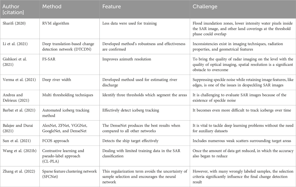
TABLE 1. Features and challenges of existing moving object detection models.

3 Methodology

In the proposed moving object detection framework, four main stages are involved, namely, pre-processing: histogram equalization technique; segmentation: weighted Otsu-based segmentation algorithm; feature extraction: GLCM, MBP, and AHME-LGBP descriptors; and object classification: ensemble deep learning technique (Bi-LSTM, RNN, and IDBN). Figure 1 shows the flow diagram of the proposed moving object detection method.

FIGURE 1

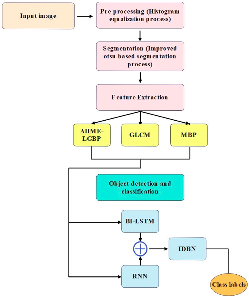
FIGURE 1. Flow diagram of the moving object detection method.

3.1 Dataset description

In this research, the MSTAR dataset is utilized for simulation. The Sandia National Laboratory SAR sensor platform collected MSTAR records. SAR object recognition is a significant issue for automatic target recognition and aerial reconnaissance in military applications. In order to assist with the creation and testing of this algorithm, MSTAR has carried out three data collections for the next-generation SAR ATR. The collections were place in November 1996, May 1997, and September 1995. The significance of the MSTAR data collection to the ATR community may make it unique. There are sufficient images for statistical significance; they are well-trusted, taken with an advanced type of radar; and they feature a range of military vehicles in a number of well-managed scenarios. The MSTAR data collection #1, Scene 1, and the MSTAR data collection #2—scenes #1, #2, and #3—both included the collection of the following dataset. An X-band STARLOS sensor operating in the spotlight mode, with a 1-foot resolution, was utilized by the Sandia National Laboratory to collect data at 15-, 17-, 30-, and 45-degree depression angles. 2S1, BDRM-2, BTR-60, D7, T62, ZIL-131, ZSU-23/4, and SLICY are among the image’s chips and JPEG files (https://www.sdms.afrl.af.mil/index.php?collection=mstar&page=targets). As part of the MSTAR initiative, the Defense Advanced Research Projects Agency and the Air Force Research Laboratory jointly financed the collection. From this dataset, only a small portion of the images are selected to process the moving object detection, and it is downloaded from https://www.kaggle.com/datasets/atreyamajumdar/mstar-dataset-8-classes. This dataset includes various target kinds, aspect angles, depression angles, serial numbers, and articulations, which is publicly accessible on the website. For example, the moving object detection images are shown in Figure 2. From the third row of Figure 2, the detected moving objects are shown with bounding boxes.

FIGURE 2

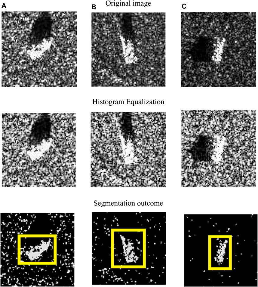
FIGURE 2. Moving object detection images. (A) Image 1. (B) Image 2. (C) Image 3.

3.2 Pre-processing

In the initial phase, the histogram equalization technique is utilized for pre-processing the input image $I$. A particular example of the more generic group of histogram remapping techniques is histogram equalization (Ulku and Camurcu, 2013). An image processing method called histogram equalization was used on computers to enhance the contrast. It achieves this enhancement by essentially extending the image’s intensity range or dispersing the most common intensity values. With this technique, the image is modified to carry out the analysis or enhance the visual quality. Mathematically, it is defined in Eq. 1. Here, $m$ denotes the total count of pixels, $v$ denotes the total count of possible intensity levels, $Y$ is the original image’s histogram or cumulative histogram properties, while $X$ represents the histogram or cumulative histogram properties of the histogram equalized image. Furthermore, $K=\mathrm{0,1,2}\dots v-1$ and $Y_K=1$. The preprocessed image is termed as $I^P$.

$\sum _{i=0}^{Y_K}M\left(i\right)=\left(\frac{m}{v}\right)\left(X_K+1\right).(1)$

3.3 Weighted Otsu-based segmentation algorithm

The preprocessed image $I^P$ is subjected to the segmentation phase via a weighted Otsu-based segmentation process. The core of Otsu’s technique is the idea, where the threshold is chosen at the gray value for which the variance among classes is the greatest or the variance within classes is the smallest (Vijay and Patil, 2016). Weighted Otsu is proposed in this work. In Eq. 2, the normalized gray-level histogram is viewed as a probability distribution, where $d_j$ represents the pixel count at step $i$, $D$ represents the overall pixel count, $Q_i$ represents the pixel, and $E$ represents the gray level.

$Q_i=\frac{d_i}{D}:\sum _{i=0}^{E-1}{Q}_i=1.(2)$

Afterward, the probabilities of class occurrences (${\vartheta }_0,{\vartheta }_1$) and class mean level (${\tau }_0,{\tau }_1$) are given in Eqs 3–6, where $G_0,G_1$ represents classes and $g$ represents the threshold level.

${\vartheta }_0=prob\left(G_0\right)=\sum _{i=0}^g{Q}_i,(3)$

${\vartheta }_1=prob\left(G_1\right)={\displaystyle \sum _{i=g+1}^{E-1}}{Q}_i,(4)$

${\tau }_0=\sum _{i=0}^{g}iprob\left(i|G_0\right),(5)$

${\tau }_1=\sum _{i=g+1}^{E-1}iprob\left(i|G_1\right).(6)$

Here, ${\vartheta }_0{\tau }_0+{{\vartheta }_1\tau }_1={\tau }_T,{\vartheta }_0+{\tau }_0=1.$

The class variances are given in Eqs 7, 8 (Vijay and Patil, 2016).

${\mu }_0^2=\sum _{i=0}^g{\left(1-{\tau }_0\right)}^{2}prob\left(i{\left|G\right.}_0\right)=\sum _{i=0}^g{\left(i-{\tau }_0\right)}^2\frac{Q_i}{{\vartheta }_0},(7)$

${\mu }_1^2=\sum _{i=\mathrm{g}+1}^{E-1}{\left(1-{\tau }_1\right)}^{2}prob\left(i{\left|G\right.}_1\right)=\sum _{i=\mathrm{g}+1}^{E-1}{\left(i-{\tau }_1\right)}^2\frac{Q_i}{{\vartheta }_i}.(8)$

As per the proposed logic, the class variance is calculated in Eqs 9, 10.

${\mu }_0^2=\sum _{i=0}^g{\left(1-{\tau }_0\right)}^{2}prob\left(i{\left|G\right.}_0\right)=\sum _{i=0}^g{\left(i-{\tau }_0\right)}^2\frac{Q_i}{{\vartheta }_i}*r,(9)$

${\mu }_1^2=\sum _{i=g+1}^{E-1}{\left(1-{\tau }_1\right)}^{2}prob\left(i{\left|G\right.}_1\right)=\sum _{i=g+1}^{E-1}{\left(i-{\tau }_1\right)}^2\frac{Q_i}{{\vartheta }_i}*r.(10)$

The Otsu method splits the image into various classes for the best thresholds and for the best segmentation, and the variances of these classes should be maximized. In order to find a threshold $t$ that maximizes the object functions, the problem is reduced to an optimization problem. This point of view is supported by the hypothesis that the variance between the classes measures the difference between two components. The difference between the two sections increases with the between-class variance. Between-class variance will reduce if we make a mistake between the objects and the background. A threshold that provides the best separation of classes in gray levels would therefore be the best threshold since increasing the between-class variance to its maximum entails reducing the chance of error to its lowest.

Here, $r$ represents weight and it is calculated according to Eq. 11, where $N$ represents the data length.

$r={\left(\underset{i=0}{\overset{N}{\pi }}\left(Q_i\right)\right)}^{\raisebox{1ex}{$1$}\!\left/ \!\raisebox{-1ex}{$N$}\right.}.(11)$

The subsequent discriminant metric is used to measure the threshold “goodness,” as indicated in Eq. 12. As per the proposed logic, the term $ww$ is included and explained in Eq. 13.

${\mu }_M={\vartheta }_0{\left({\tau }_0-{\tau }_T\right)}^2\times ww+{\vartheta }_1{\left({\tau }_1-{\tau }_T\right)}^2\times \left(1-ww\right).(12)$

Here,

$ww=\frac{{\tau }_0}{{\tau }_0+{\tau }_1}.(13)$

The variance between classes is the variance between the mean of the members of classes. $ww$ is referred as weighted Otsu, which improves the image segmentation effect clearly. The computation for $\tau$ and $\vartheta$ is simplified because the formulas for the class variance are modified and expressed in a recursive form. Consequently, the threshold with the lowest within-class variance also has the greatest variance between classes. As a result, it can also be used to determine the best threshold, and because it is easier, it is a much better method to employ.

3.4 Feature extraction

After segmentation, the features like AHME-LGBP-, GLCM-, and MBP-based features are extracted.

3.4.1 AHME-LGBP

AHME-LGBP is the variant of LGBP with the estimation of weighted harmonic mean in pattern extraction. The Gabor features’ micro-patterns are encoded using the LBP operator. The LGBP (Zhang et al., 2007) operator is the result of combining the Gabor and LBP operators. First, the Gabor filter is applied to the input segmented image. Then, LBP is applied to the Gabor filter resultant image. In the segmented image, it is assumed that the eight neighbors of the center pixel placed at $\left(a_l,b_l\right)$ be $\left(a_r,b_r\right)$ with $r=\mathrm{0,1,2}\dots 7$. Formally, the LGBP pattern at $\left(a_l,b_l\right)$ is defined as in Eq. 14. Here, $f$ represents the scale parameter, $\mathrm{\Psi }$ represents the orientation parameter, $a,b$ denotes the direction, and $W\left(a_r,b_r\right)$ denotes the intensity of an image.

$LGB{P}_{f,\psi }\left(a_l,b_l\right)=\sum _{r=0}^{7}K\left(W_{f,\psi }\left(a_r,b_r\right)-W_{f,\psi }\left(a_l,b_l\right)\right){.2}^r.(14)$

Therefore, Eq. 15 is stated as

$K\left(x\right)=\left\{\begin{array}{c}1,x\ge 0,\\ 0,x<0.\end{array}\right.(15)$

According to the recommended method, modified LGBP, named as AHME-LGBP, is given in Eq. 16. It uses the median within the image patch instead of the central pixel as the local threshold to enhance noise robustness, where $a_m,b_m$ are the mean values and $wi$ represents the weighted harmonic mean.

$AHME-LGB{P}_{f,\psi }\left(a_l,b_l\right)=\sum _{r=0}^{7}K\left(W_{f,\psi }\left(a_r,b_r\right)-W_{f,\psi }\left(a_m,b_m\right)\right){.2}^r,a_m=\frac{\sum _{i=0}^{7}wi}{\sum _{i=0}^7\frac{wi}{ai}}.(16)$

3.4.2 GLCM

GLCM is an effective feature descriptor that analyzes the spatial relationship between two pixels to determine the texture of a picture. The simultaneous existence of pixel pairs can be identified because the distance and orientation between pixels are changed. In GLCM, 14 different kinds of features are presented. Some of the textural characteristics are drawn from this. The textural data obtained from GLCM served as the foundation for the effective description. GLCM (Mohanaiah et al., 2013) has proven to be a popular statistical method of extracting the textural feature from images. Four important features, namely, the angular second moment (energy), correlation, entropy, and inverse difference moment are extracted.

The instantaneous occurrence probability of two pixels is specified as $P\left(i,j,\delta ,\theta \right)$. It comprises the pixel with grayscales $i$ and $j$ as $f\left(x,y\right)$ and $\left(x+\Delta x,y+\Delta y\right)$, respectively; $\theta$ is explained as declination; and the distance is referred as $\delta$. The arithmetic formula for instantaneous occurrence probability $P\left(i,j,\delta ,\theta \right)$ is expressed in Eq. 17.

$P\left(i,j,\delta ,\theta \right)=\left\{\begin{array}{c}\left|\left[\left(x,y\right),\left(x+\Delta x,y+\Delta y\right)\right]\right|f\left(x,y\right)=i,\\ \left(x,y\right),f\left(x+\Delta x,y+\Delta y\right)=j;x=\mathrm{0,1},..,N_x-1;\\ y=\mathrm{0,1},..,N_y-1\end{array}\right\},(17)$

where $i,j=\mathrm{0,1},\dots L-1;L$ is signified as a gray-level image; image pixel coordinates are indicated as $x$ and $y$; and $N_x$ and $N_y$ are referred to as the numbers of columns and rows, respectively.

a) Angular second moment (energy): It is the total of the squares of GLCM entries. It determines the texture of the segmented image ($S^{img}$). The mathematical expression is given in Eq. 18, where $E\left(i,j\right)$ is the ${\left(i,j\right)}^{th}$ entry in GLCM and $Q$ denotes the gray tone.

$\text{Angular\hspace{1em}second\hspace{1em}moment}={\sum _{i=0}^{Q-1}\sum _{j=0}^{Q-1}\left(S{}_{i,j}^{img}\right)}^2.(18)$

b) Correlation: It computes the correction between the current pixel and neighboring pixel in the segmented image. For a positively correlated image, correlation = 1, and for a negatively correlated image, correlation = −1. The expression for correlation is shown in Eq. 19, in which ${\sigma }_x,{\sigma }_y$ and ${\mu }_{x,}{\mu }_y$ are the standard deviations and mean of $S_x^{img}$ and $S_y^{img}$, respectively.

$Correlation=\frac{\sum _i\sum _j\left(ij\right)S_{i,j}^{img}-{\mu }_x{\mu }_y}{{\sigma }_x{\sigma }_y}.(19)$

c) Entropy: It defines the required count of information for compressing $S^{img}$, and it is shown in Eq. 20.

$Entropy=-\sum _i\sum _j{S}_{i,j}^{img}{\log }_2{S}_{i,j}^{img}.(20)$

d) Inverse difference moment: It is the local homogeneity. When the local gray level is uniform and the inverse GLCM is high, the inverse difference moment is said to be high. The numerical expression for the inverse difference moment is shown in Eq. 21.

$\text{Inverse\hspace{1em}differ}\mathrm{e}\text{nce\hspace{1em}moment}=\frac{{\displaystyle \sum _i}{\displaystyle \sum _j}{S}_{i,j}^{img}}{1+{\left(i-j\right)}^2}(21)$

3.4.3 MBP

MBP (Hafiane et al., 2015) is related to LBP, but rather than using the central pixel as the local threshold, it utilizes the median inside the image patch to provide improved noise robustness and increased sensitivity to microstructures. Improved MBP is given in Eq. 22, where $\phi \left(o,p\right)$ represents the median inside the image patch, $f_s$ represents the gray value of pixel at position index $s$ and $J$ represents the binary threshold.

$MB{P}_{U,V}\left(o,p\right)={\displaystyle \sum _{s\in N_p\left(o,p\right)}}{2}^{s}J\left(f_s-\phi \left(o,p\right)\right).(22)$

Every object detection system needs feature extraction, which is a crucial part of these systems. Feature extraction is the process of mapping the image pixels into the feature space. The extracted AHME-LGBP, GLCM, and MBP features are collected and subjected to a detection process for detecting the moving objects. The final feature set is denoted as $F^S$, and it is shown in Eq. 23.

$F^S=\left[MB{P}_{U,V}GLCMAHME-LGBP\right].(23)$

To identify and categorize an object, similar features are combined to create a feature vector. Moving object detection deals with detecting the instances of morphological objects of a certain class. Therefore, the proposed method is superior in the feature extraction method, and these three types of features have significant impact on the final experimental results, which is demonstrated in the upcoming Section 4. Figure 3 shows the feature importance analysis, and the extracted 3,278 feature values are given to the ensemble deep learning techniques Bi-LSTM, RNN, and IDBN for moving object classification in SAR images.

FIGURE 3

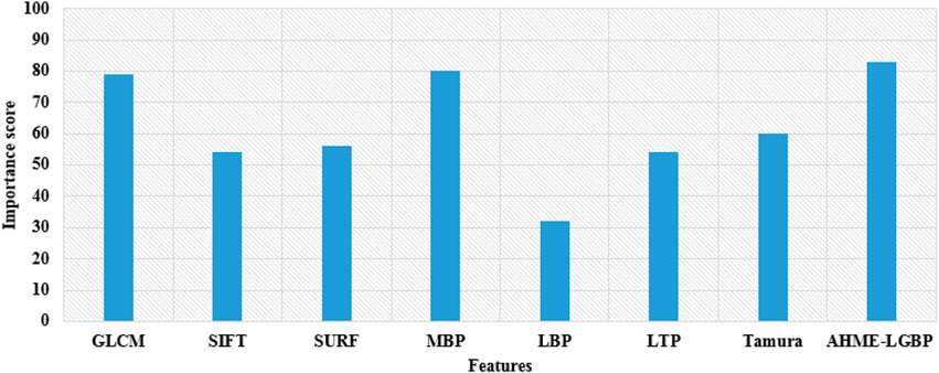
FIGURE 3. Feature importance analysis.

3.5 Object classification

In this phase, the object can be classified using the ensemble deep learning method that trains with the extracted features $F^S$. Here, Bi-LSTM, RNN, and IDBN are involved. The working strategy is as follows:

• The input features are processed with Bi-LSTM and RNN.

• The generating outputs obtained from the above phases are averaged and given as the input to IDBN to attain the final result.

3.5.1 Bi-LSTM

In contrary to the conventional unidirectional LSTM, Bi-LSTM (Ye et al., 2019) takes into account all the information obtained from both the prior and subsequent segments. The formulations are shown in Eqs 24–28.

$I_t=\lambda \left(K_I*\left[h_{t-1},X_t\right]+f_I\right),(24)$

$C_t=\lambda \left(K_C*\left[h_{t-1},X_t\right]+f_C\right),(25)$

$g_t=\lambda \left(K_g*\left[h_{t-1},X_t\right]+f_g\right),(26)$

$B_t=C_t*B_{t-1}+I_t*\tanh \left(K_B*\left[h_{t-1},X_t\right]+f_B\right),(27)$

$h_t=g_t*\tanh \left(B_t\right),(28)$

where $I_t$, $C_t$, $g_t$, and $B_t$ denote the output of the input gate, forget gate, output gate, and cell at time $t$, respectively. The sigmoid activation function is represented by $\lambda$; $X_t$ and $h_t$ denote the input vector and output layer vector at time $t$, respectively; $K_I$ and $f_I$ are the weight matrix and bias vector corresponding to the input gate, respectively. The weight matrix and bias vector for the forget gate are $K_C$ and $f_C$, that for the output gate are $K_g$ and $f_g$, and that for the cell are $K_B$ and $f_B$, respectively.

The Bi-LSTM structure consists of two parallel LSTM layers in both forward and reverse directions. The two parallel LSTM layers function similar to traditional LSTM neural networks. They begin and end the sentence, allowing them to store information from both directions. For $t$ time step, two parallel layers in both directions manage the input data from their opposite directions. Then, the output of the sum of the hidden state vectors is described in Eq. 29.

$h_t=k_1\overrightarrow{h_t}+k_2\overrightarrow{h_t}+B.(29)$

Here, $\overrightarrow{h_t}$ and $\overrightarrow{h_t}$ denote the output outcomes of the two parallel LSTM layers in both forward and reverse directions, and $k_1$ and $k_2$ denote the weight parameters of two parallel LSTM layers in both forward and reverse directions, respectively.

3.5.2 RNN

Due to the fact that RNNs are the only neural networks (NNs) with an internal memory, they are a strong and reliable type of NN and one of the most promising networks that is currently being used. The information on RNN loops back on itself. It takes into account both the current input and the learning it has learned from the inputs it has already received when making decisions.

RNN (Park et al., 2020) is defined in Eq. 30, where $s_t$ represents the predicted result, $t$ represents time, $l_1$ represents the real value, and $f_t$ represents the hidden layer, which is calculated in Eq. 31, where $l_2,l_3$ represents the real values, $u_t$ represents the input layer, and $f_{t-1}$ represents the preceding hidden layer.

$s_t=l_1{f}_t+m_s,(30)$

$f_t=\tanh \left(l_2{u}_t+l_3{f}_{t-1}+m_f\right).(31)$

The method of discovering actual values can reduce the error value $Er$ using machine learning (ML) depending on RNN.

3.5.3 Improved DBN

DBN (Wang et al., 2021) is referred as a probabilistic generation technique, which was stacked with restricted Boltzmann machines (RBMs). There are two layers in RBMs: one that is visible and the other that is hidden. There are no links within any of the levels; rather, the links among hidden and visible layers are only present. Data are fed into the first RBM’s visible layer, and the result of the preceding RBM becomes the input for the subsequent RBM.

There are two phases to the learning process. Each RBM is initially trained layer by layer using the unsupervised greedy approach. It is possible to retrieve each RBM’s parameter at this step. Supervised back-propagation is employed for fine-tuning overall networks. If RBM includes neurons $e$ in the visible layer and neurons $f$ in the hidden layer, the state’s energy function is provided in Eq. 32.

$A\left(c,d|\varphi \right)=-\sum _{i=1}^e{g}_i{c}_i-\sum _{j=1}^f{h}_i{d}_j-\sum _{i=1}^e\sum _{j=1}^f{c}_i{k}_{ij}{d}_j.(32)$

The joint probability of $c,d$ is attained in Eq. 33, where $c,d$ represents the visible and hidden layer and $g,h$ represents the visible layer offset.

$prob\left(c,d|\varphi \right)=\raisebox{1ex}{$e^{-A\left(c,d|\varphi \right)}$}\!\left/ \!\raisebox{-1ex}{$Q\left(\varphi \right)$}\right.,Q\left(\varphi \right)=\sum _{c,d}{e}^{-A\left(c,d|\varphi \right)}.(33)$

The probability of hidden layer’s activation function is specified in Eq. 34, and the probability of visible layer’s activation function is specified in Eq. 35.

$prob\left(d_j=1|c,\rho \right)=\lambda \left(h_i+\sum _i{c}_i{k}_{ij}\right),(34)$

$prob\left(c_i=1|d,X\right)=\lambda \left(g_i+\sum _j{k}_{ij}{d}_j\right).(35)$

According to the improved version, the leaky rectified linear unit (ReLU) activation function is used. Leaky ReLU acts as a default activation function for several kinds of NN since using it makes a model simpler to train and frequently results in greater performance. Moreover, a new loss evaluation is given with the IDBN version, and cross-entropy is calculated, which is specified in Eq. 36.

$E=-\frac{1}{W}\sum _{i=1}^W\left[r_n\log \left(S\left(z_n\right)-\left(1-r_n\right)\log \left(1-S\left(z_n\right)\right)\right)\right].(36)$

The parameters considered in the ensemble deep learning techniques Bi-LSTM, RNN, and IDBN are as follows: the batch size is 150, the loss function is cross-entropy, the learning rate is 0.0025, the number of hidden layers is 32, the number of epochs is 100, the Lambda loss amount is 0.0015, and activation functions are sigmoid and tangent. Figure 4 depicts the overall classification process. The numerical analysis of the proposed method is discussed in Section 4.

FIGURE 4

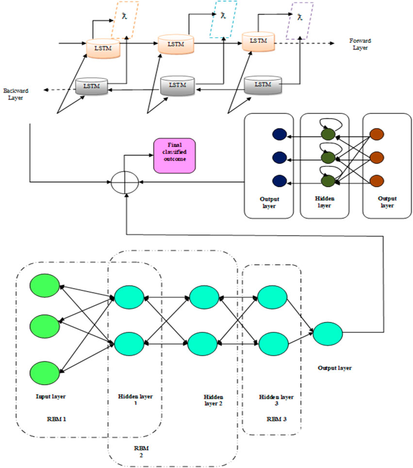
FIGURE 4. Deep ensemble model for detecting the objects from SAR images.

4 Results and discussions

4.1 Simulation procedure

The developed moving object detection and classification using SAR images with an ensemble model is implemented in MATLAB, and the results are verified. Moreover, the ensemble method is computed over the conventional classifiers, like CNN, SVM, random forest (RF), bidirectional gated recurrent unit (Bi-GRU), FCOS (Sharifi, 2020), RCNN (Sun et al., 2021), DTCDN (Li et al., 2021), and deep maxout. Furthermore, evaluation is done based on positive measures, negative measures, and other measures for diverse learning percentage, ranging from 60, 70, 80, and 90, respectively. The evaluation measures are as follows: false discovery rate (FDR), false positive rate (FPR), Matthews correlation coefficient (MCC), negative predictive values (NPVs), false negative rate (FNR), sensitivity, specificity, precision, accuracy, and F-measure are utilized for evaluating the proposed models’ effectiveness, which are mathematically mentioned in Eqs 37–47. Here, true positives are referred as $TP$, true negatives are referred as $TN$, false positives are referred as $FP$, and false negatives are denoted as $FN$.

$FDR=\frac{FP}{FP+TP},(37)$

$FPR=\frac{FP}{FP+TN},(38)$

$MCC=\frac{TP*TN-FP*FN}{\sqrt{\left(TP+FP\right)*\left(TP+FN\right)*\left(TN+FP\right)*\left(TN+FN\right)}},(39)$

$NPV=\frac{TN}{TN+FN},(40)$

$FNR=\frac{FN}{FN+TP},(41)$

$Sensitivity=\frac{TP}{FN+TP},(42)$

$Specificity=\frac{TN}{TN+FP},(43)$

$\mathrm{Pr}ecision=\frac{TP}{TP+FP},(44)$

$Accuracy=\frac{TP+TN}{TP+TN+FP+FN},(45)$

$F-measure=\frac{2TP}{2TP+FP+FN},(46)$

$ErrorRate=100-Accuracy.(47)$

4.2 Analysis on positive measures

The performance of the ensemble method is evaluated over the established methods regarding various metrics. The results of positive measures on the ensemble method over traditional methods are shown in Figure 5. By reviewing the entire graphs, the ensemble model has obtained better outcomes than extant approaches. Figure 5A shows that the ensemble method has achieved a better detection accuracy of approximately 0.98, which is improved than the conventional methodologies, such as FCOS is 0.78, faster RCNN is 63.56%, CNN is 0.87, SVM is 0.90, RF is 0.48, Bi-GRU is 0.89, DTCDN is 0.83, and deep maxout is 0.39, respectively, at the 90% of learning percentage. Additionally, Figure 5B shows that the precision measure has yielded a higher value of 0.97 for the ensemble scheme when the learning rate is 70%, which is much superior to the values attained by traditional methods, such as FCOS, faster RCNN, CNN, SVM, RF, Bi-GRU, DTCDN, and deep maxout.

FIGURE 5

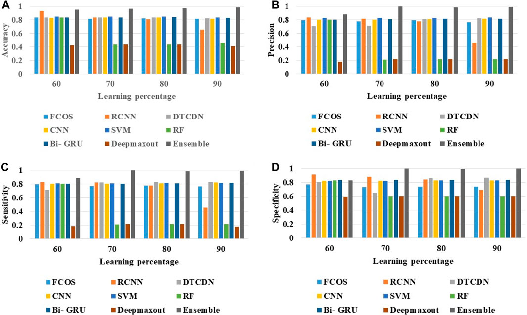
FIGURE 5. Analysis on positive measures: ensemble method over other traditional schemes. (A) Accuracy. (B) Precision. (C) Sensitivity. (D) Specificity.

Figure 5C shows that the ensemble approach has offered a higher value over other schemes, i.e., the ensemble approach has attained a high sensitivity of 0.94 (in the 70% of learning rate), while models like FCOS, faster RCNN, SVM, RF, DTCDN, and Bi-GRU have maintained a relatively minimal sensitivity of 0.65, 0.79, 0.82, 0.80, 0.83, and 0.81, respectively. Finally, the specificity of the ensemble strategy is approximately 0.94, in the 90% of learning percentage. Therefore, it confirms the feasibility of the ensemble model for the identification and categorization of moving objects.

4.3 Analysis on negative measures

The performance of the ensemble scheme over the extant methods regarding FDR, FNR, and FPR is described in this section. Figure 6 shows the negative measure analysis of the ensemble work is contrasted over other methods. Furthermore, Figures 6A–C show that the measures, like FDR, FNR, and FPR of the adopted method, obtained better outcomes than other conventional classifiers. The FDR of 0.02 is obtained by the ensemble model at 90% of the learning percentage. On the other hand, the compared models, like FCOS, faster RCNN, CNN, SVM, RF, DTCDN, and Bi-GRU, have obtained relatively higher FDR values of 0.28, 0.45, 0.16, 0.14, 0.73, 0.09, and 0.12, respectively. Likewise, for an FNR metric, a lesser error of 0.03 is achieved by the ensemble model at 70% of the learning percentage. The FPR of the Ensemble method is 0.01, which is superior to FCOS (0.13), faster RCNN (0.076), CNN (0.11), SVM (0.09), RF (0.38), DTCDN (0.078), and Bi-GRU (0.08), at the learning percentage of 70. Thus, the ensemble model’s superiority over other conventional classifiers in terms of negative metrics is demonstrated.

FIGURE 6

FIGURE 6. Analysis on negative measures: ensemble method over other traditional schemes. (A) FDR; (B) FNR; and (C) FPR.

4.4 Analysis on other measures

The analysis is done by varying the learning percentage that ranges from 60 to 90 with respect to metrics like F-measure, MCC, and NPV, which is shown in Figure 7. By analyzing Figure 7A, in the 70% of learning rate, the worst performance is given by the RF and deep maxout algorithms, whereas the ensemble method gained the highest F-measure of approximately 0.97. Similarly, the ensemble strategy attained the highest MCC of 0.94, which is preferable than the other classifiers, like FCOS, faster RCNN, CNN, SVM, RF, Bi-GRU, DTCDN, and deep maxout, respectively. In accordance with the NPV measure analysis, the ensemble model has recorded the highest NPV value, which is 0.83, 0.98, 0.94, and 0.95, when the learning rate is 60, 70, 80, and 90, respectively. Therefore, the ensemble method provides enhanced object detection performance due to the significant improvement of the other measures.

FIGURE 7

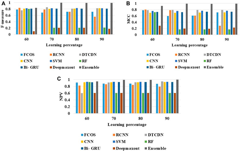
FIGURE 7. Analysis on negative measures: ensemble method over other traditional schemes: (A) F-measure; (B) MCC; and (C) NPV.

Here, the proposed method is superior in the feature extraction method, and the three types of features have the same impact on the final experimental results.

4.5 Ablation study

Table 2 shows the ablation study of the ensemble work, the model with conventional LGBP, model without segmentation, model with conventional DBN, and model without feature extraction. The precision of the ensemble method is 0.87, the model with conventional LGBP is 0.81, model without segmentation is 0.77, model with conventional DBN is 0.83, and model without feature extraction is 0.80. Similarly, the accuracy obtained by the proposed model is 0.10, 0.8, 0.7, and 0.11 superior to the model with conventional LGBP, model without segmentation, model with conventional DBN, and model without feature extraction, respectively. Additionally, the FDR of the ensemble model is 0.89, 0.83, 0.86, and 0.87 better than the model with conventional LGBP, model without segmentation, model with conventional DBN, and model without feature extraction, respectively. Moreover, in terms of the error rate, the proposed ensemble method achieved 0.054, which is better than the conventional methods shown in Table 2. Thus, the robustness of the ensemble model is verified successfully.

TABLE 2

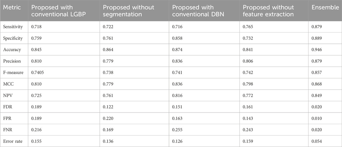
TABLE 2. Ablation study on the ensemble method, with conventional LGBP, without segmentation, and with conventional DBN.

4.6 Statistical analysis with respect to errors

Due to the stochastic character of the optimization process, it is repeatedly run to determine the final outcomes in terms of statistical analysis. Moreover, it was evaluated by using the different (five) types of case scenarios, such as mean, best, standard deviation, median, and worst, and the outcomes are summarized in Table 3. Here, the ensemble method recorded the lowest error rate than the other existing schemes. In the mean-case scenario analysis, the ensemble method acquired the error value of 0.032, whereas the compared method FCOS, faster RCNN, CL-PLA, SFCNet, CNN, SVM, RF, Bi-GRU, DTCDN, and deep maxout scored a very high error rate of 0.170, 0.181, 0.35, 0.36, 0.132, 0.113, 0.427, 0.126, 0.132, and 0.541, respectively. Simultaneously, in the median- and best-case scenario analysis, the ensemble method yielded the lowest error value of 0.029 and 0.015, respectively. Thus, it may be concluded that the ensemble strategy is suitable for detecting and classifying the moving object.

TABLE 3

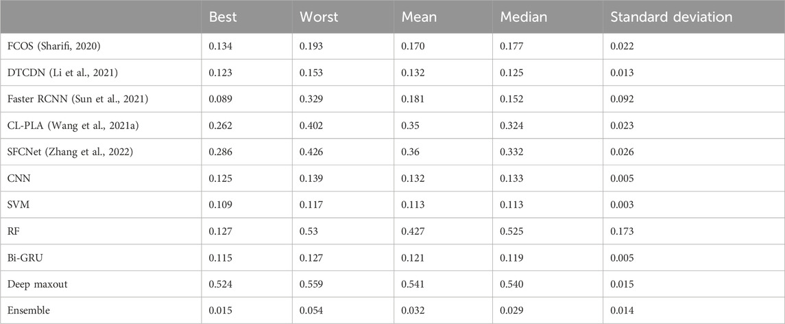
TABLE 3. Statistical analysis with respect to the error between actual and predicted images.

4.7 Segmentation analysis

Table 4 shows the segmentation analysis outcomes. The improved Otsu-based segmentation process is compared with the conventional Otsu, Fuzzy C-Means algorithm (FCM), k-means methods, CL-PLA (Wang et al., 2021), and SFCNet (Zhang et al., 2022). On analyzing the results, the accuracy of the proposed work is 0.968, which is better than the existing conventional Otsu (0.854), FCM (0.775), k-means methods (0.865), CL-PLA (0.872), and SFCNet (0.881). The F-measure of the improved Otsu work is 0.863, and it is 15.06%, 6.03%, and 16.22% better than the extant Otsu, FCM, and k-means methods. Similarly, other measures also achieve superior results compared to the existing ones. Thus, the effectiveness of the improved Otsu-based segmentation process is validated.

TABLE 4

TABLE 4. Segmentation accuracy analysis of the proposed and conventional segmentation methods.

Table 5 shows the target detection rate analysis of the proposed method. Table 5 shows that the proposed (improved Otsu) method has achieved better results in terms of recall (0.854), F1-measure (0.871), mean average precision (0.846), and DICE (0.905). Figure 8 shows the visualization of the moving object detection.

TABLE 5

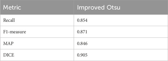
TABLE 5. Target detection rate analysis of the proposed method.

FIGURE 8

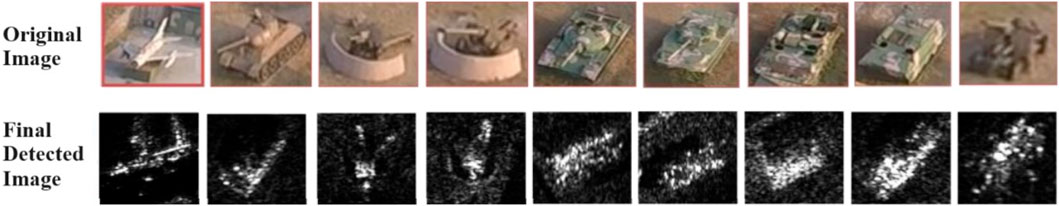
FIGURE 8. Visualization of moving object detection.

4.8 Analysis of moving target detection

In this research, the images are taken from the MSTAR dataset, where the images are moved according to the time frame manner. Therefore, the following sample images are moving in a time frame, which is shown in Figure 9.

FIGURE 9

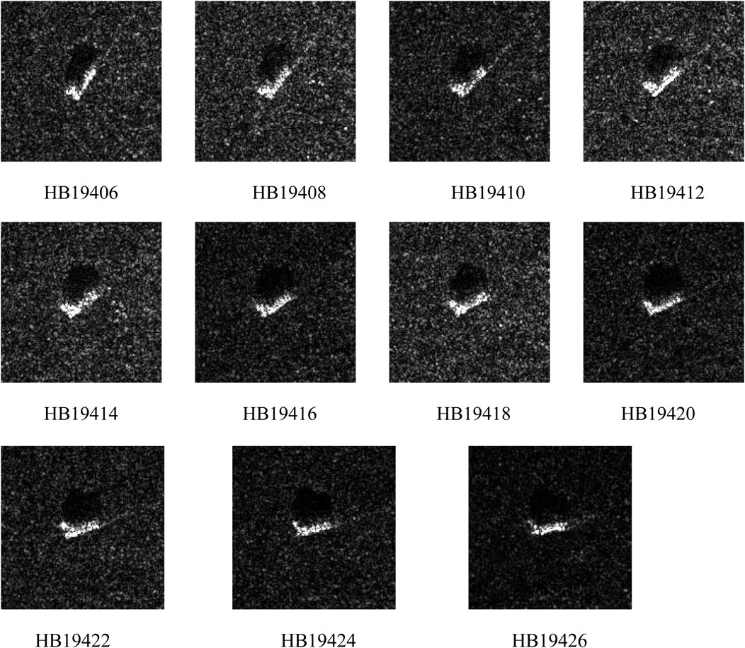
FIGURE 9. Sample images of moving object detection.

Moving objects are identified by moving object detection systems as groups of bounding boxes based on the variations in the images (or motions) between frames. This paper mainly focuses on moving target detection; therefore, the data on large scenes and other moving target data have been added to verify the feasibility of the algorithm. Figure 10 displays the detected moving portion (bounding boxes) from the given input data. Figure 10 shows that moving portions are detected with the indication of a bounding box.

FIGURE 10

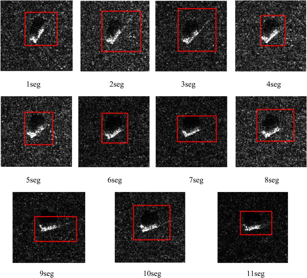
FIGURE 10. Object detection with a bounding box.

The detection and tracking of moving objects can be viewed as a lower-level vision task to achieve higher levels of image understanding. Furthermore, to demonstrate the effectiveness of the proposed method, the visualization of heatmaps is included in the middle layer of the network, which is shown in Figure 11.

FIGURE 11

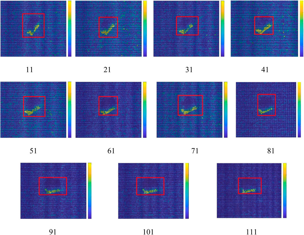
FIGURE 11. Visualization with heatmaps.

5 Conclusion

In this manuscript, an effective moving object detection and classification model is developed that includes four stages, namely pre-processing, segmentation, feature extraction, and classification. In the first step, the input SAR image is pre-processed using a histogram equalization technique. Then, the weighted Otsu-based segmentation algorithm is performed for segmenting the RoI from the pre-processed input images. Then, features like GLCM, MBP, and AHME-LGBP are extracted. Classification is the last step; here, the objects are classified by employing an effective ensemble deep learning technique. In the classification stage, Bi-LSTM and RNN classifiers are averaged, which considers extracted features as an input. Both classifiers' averaged output is then fed to IDBN to obtain the final predicted output. Compared to the conventional deep maxout approach, the ensemble deep learning technique obtained an error value of 0.032 in the mean-case scenario. Simultaneously, the ensemble deep learning technique achieved the lowest error value of 0.029 and 0.015 in the median- and best-case scenario analyses. In future, this research will be further extended by analyzing various methodologies to enhance the error value.

Data availability statement

The original contributions presented in the study are included in the article/Supplementary Material; further inquiries can be directed to the corresponding author.

Author contributions

RP: data curation, formal analysis, methodology, software, validation, and writing–original draft. PK: data curation, formal analysis, methodology, software, validation, and writing–original draft. W-CL: funding acquisition, methodology, project administration, resources, supervision, and writing–review and editing. PB: conceptualization, investigation, methodology, supervision, visualization, and writing–review and editing.

Funding

The authors declare that no financial support was received for the research, authorship, and/or publication of this article.

Conflict of interest

The authors declare that the research was conducted in the absence of any commercial or financial relationships that could be construed as a potential conflict of interest.

Publisher’s note

All claims expressed in this article are solely those of the authors and do not necessarily represent those of their affiliated organizations, or those of the publisher, the editors, and the reviewers. Any product that may be evaluated in this article, or claim that may be made by its manufacturer, is not guaranteed or endorsed by the publisher.

References

Andrea, R., and Delrieux, C. (2021). Multithresholding techniques in SAR image classification. Remote Sens. Appl. Soc. Environ. 23, 100540. doi:10.1016/j.rsase.2021.100540

CrossRef Full Text | Google Scholar

Bai, J., Li, S., Huang, L., and Chen, H. (2021). Robust detection and tracking method for moving object based on radar and camera data fusion. IEEE Sens. J. 21 (9), 10761–10774. doi:10.1109/JSEN.2021.3049449

CrossRef Full Text | Google Scholar

Baiju, P. S., and George, S. N. (2020). An automated unified framework for video deraining and simultaneous moving object detection in surveillance environments. IEEE Access 8, 128961–128972. doi:10.1109/ACCESS.2020.3008903

CrossRef Full Text | Google Scholar

Balajee, J., and Durai, M. A. S. (2021). Detection of water availability in SAR images using deep learning architecture. Int. J. Syst. Assur. Eng. Manage. doi:10.1007/s13198-021-01152-5

CrossRef Full Text | Google Scholar

Barbat, M. M., Rackow, T., Wesche, C., Hellmer, H. H., and Mata, M. M. (2021). Automated iceberg tracking with a machine learning approach applied to SAR imagery: a Weddell sea case study. ISPRS J. Photogramm. Remote Sens. 172, 189–206. doi:10.1016/j.isprsjprs.2020.12.006

CrossRef Full Text | Google Scholar

Bi, H., Deng, J., Yang, T., Wang, J., and Wang, L. (2021). CNN-based target detection and classification when sparse SAR image dataset is available. IEEE J. Sel. Top. Appl. Earth Obs. Remote Sens. 14, 6815–6826. doi:10.1109/JSTARS.2021.3093645

CrossRef Full Text | Google Scholar

Chen, Y., Wang, J., Zhu, B., Tang, M., and Lu, H. (2019). Pixelwise deep sequence learning for moving object detection. IEEE Trans. Circuits Syst. Video Technol. 29 (9), 2567–2579. doi:10.1109/TCSVT.2017.2770319

CrossRef Full Text | Google Scholar

Eltantawy, A., and Shehata, M. S. (2019a). An accelerated sequential PCP-based method for ground-moving objects detection from aerial videos. IEEE Trans. Image Process 28 (12), 5991–6006. doi:10.1109/TIP.2019.2923376

PubMed Abstract | CrossRef Full Text | Google Scholar

ElTantawy, A., and Shehata, M. S. (2019b). KRMARO: aerial detection of small-size ground moving objects using kinematic regularization and matrix rank optimization. IEEE Trans. Circuits Syst. Video Technol. 29 (6), 1672–1686. doi:10.1109/TCSVT.2018.2843761

CrossRef Full Text | Google Scholar

Fu, J., Sun, X., Wang, Z., and Fu, K. (2021). An anchor-free method based on feature balancing and refinement network for multiscale ship detection in SAR images. IEEE Trans. Geosci. Remote Sens. 59 (2), 1331–1344. doi:10.1109/TGRS.2020.3005151

CrossRef Full Text | Google Scholar

Gishkori, S., Daniel, L., Gashinova, M., and Mulgrew, B. (2021). Imaging moving targets for a forward scanning SAR without radar motion compensation. Signal Process. 185, 108110. doi:10.1016/j.sigpro.2021.108110

CrossRef Full Text | Google Scholar

Hafiane, A., Palaniappan, K., and Seetharaman, G. (2015). Joint adaptive median binary patterns for texture classification. Pattern Recognit. 48 (8), 2609–2620. doi:10.1016/j.patcog.2015.02.007

CrossRef Full Text | Google Scholar

Han, L., Ran, D., Ye, W., Yang, W., and Wu, X. (2020). Multi-size convolution and learning deep network for SAR ship detection from scratch. IEEE Access 8, 158996–159016. doi:10.1109/ACCESS.2020.3020363

CrossRef Full Text | Google Scholar

Hong, Z., Yang, T., Tong, X., Zhang, Y., Jiang, S., Zhou, R., et al. (2021). Multi-scale ship detection from SAR and optical imagery via A more accurate YOLOv3. IEEE J. Sel. Top. Appl. Earth Obs. Remote Sens. 14, 6083–6101. doi:10.1109/JSTARS.2021.3087555

CrossRef Full Text | Google Scholar

Javed, S., Mahmood, A., Al-Maadeed, S., Bouwmans, T., and Jung, S. K. (2019). Moving object detection in complex scene using spatiotemporal structured-sparse RPCA. IEEE Trans. Image Process 28 (2), 1007–1022. doi:10.1109/TIP.2018.2874289

CrossRef Full Text | Google Scholar

Li, J., Pan, Z. M., Zhang, Z. H., and Zhang, H. (2019). Dynamic ARMA-based background subtraction for moving objects detection. IEEE Access 7, 128659–128668. doi:10.1109/ACCESS.2019.2939672

CrossRef Full Text | Google Scholar

Li, X., Du, Z., Huang, Y., and Tan, Z. (2021). A deep translation (GAN) based change detection network for optical and SAR remote sensing images. ISPRS J. Photogramm. Remote Sens. 179, 14–34. doi:10.1016/j.isprsjprs.2021.07.007

CrossRef Full Text | Google Scholar

Meng, W., Wang, L., Du, A., and Li, Y. (2020). SAR image change detection based on data optimization and self-supervised learning. IEEE Access 8, 217290–217305. doi:10.1109/ACCESS.2020.3042017

CrossRef Full Text | Google Scholar

Mohanaiah, P., Sathyanarayana, P., and GuruKumar, L. (2013). Image texture feature extraction using GLCM approach. Int. J. Sci. Res. Publ. 3 (5), 1–5.

Google Scholar

Ou, X., Yan, P., Zhang, Y., Tu, B., Zhang, G., Wu, J., et al. (2019). Moving object detection method via ResNet-18 with encoder-decoder structure in complex scenes. IEEE Access 7, 108152–108160. doi:10.1109/ACCESS.2019.2931922

CrossRef Full Text | Google Scholar

Park, J., Yi, D., and Ji, S. (2020). Analysis of recurrent neural network and predictions. Symmetry 12 (4), 615. doi:10.3390/sym12040615

CrossRef Full Text | Google Scholar

Saha, S., Bovolo, F., and Bruzzone, L. (2021). Building change detection in VHR SAR images via unsupervised deep transcoding. IEEE Trans. Geosci. Remote Sens. 59 (3), 1917–1929. doi:10.1109/TGRS.2020.3000296

CrossRef Full Text | Google Scholar

Shahbaz, A., and Jo, K.-H. (2020). “Moving object detection based on deep atrous spatial features for moving camera,” in 2020 IEEE 29th International Symposium on Industrial Electronics (ISIE), Delft, Netherlands, 17-19 June 2020 (IEEE), 67–70. doi:10.1109/ISIE45063.2020.9152237

CrossRef Full Text | Google Scholar

Sharifi, A. (2020). Flood mapping using relevance vector machine and SAR data: a case study from aqqala, Iran. J. Indian Soc. Remote Sens. 48 (9), 1289–1296. doi:10.1007/s12524-020-01155-y

CrossRef Full Text | Google Scholar

Shi, Y., Du, L., and Guo, Y. (2021). Unsupervised domain adaptation for SAR target detection. IEEE J. Sel. Top. Appl. Earth Obs. Remote Sens. 14, 6372–6385. doi:10.1109/JSTARS.2021.3089238

CrossRef Full Text | Google Scholar

Sun, Z., Dai, M., Leng, X., Lei, Y., Xiong, B., Ji, K., et al. (2021). An anchor-free detection method for ship targets in high-resolution SAR images. IEEE J. Sel. Top. Appl. Earth Obs. Remote Sens. 14, 7799–7816. doi:10.1109/JSTARS.2021.3099483

CrossRef Full Text | Google Scholar

Ulku, E. E., and Camurcu, A. Y. (2013). “Computer aided brain tumor detection with histogram equalization and morphological image processing techniques,” in 2013 International Conference on Electronics, Computer and Computation (ICECCO), Ankara, Turkey, 07-09 November 2013 (IEEE), 48–51. doi:10.1109/ICECCO.2013.6718225

CrossRef Full Text | Google Scholar

Verma, U., Chauhan, A., Pai, M. M. M., and Pai, R. (2021). DeepRivWidth: deep learning based semantic segmentation approach for river identification and width measurement in SAR images of Coastal Karnataka. Comput. Geosci. 154, 104805. doi:10.1016/j.cageo.2021.104805

CrossRef Full Text | Google Scholar

Vijay, P. P., and Patil, N. C. (2016). Gray scale image segmentation using OTSU thresholding optimal approach. J. Res. 2 (5), 20–24.

Google Scholar

Wang, C., Gu, H., and Su, W. (2021a). SAR image classification using contrastive learning and pseudo-labels with limited data. IEEE Geoscience Remote Sens. Lett. 19, 1–5. doi:10.1109/lgrs.2021.3069224

CrossRef Full Text | Google Scholar

Wang, Y., Yang, G., Xie, R., Liu, H., Liu, K., and Li, X. (2021b). An ensemble deep belief network model based on random subspace for NO_x concentration prediction. ACS Omega 6 (11), 7655–7668. doi:10.1021/acsomega.0c06317

PubMed Abstract | CrossRef Full Text | Google Scholar

Ye, H., Cao, B., Peng, Z., Chen, T., Wen, Y., and Liu, J. (2019). Web services classification based on wide & Bi-LSTM model. IEEE Access 7, 43697–43706. doi:10.1109/ACCESS.2019.2907546

CrossRef Full Text | Google Scholar

Yu, K., Qi, X., Sato, T., Myint, S. H., Wen, Z., Katsuyama, Y., et al. (2020). Design and performance evaluation of an AI-based W-band suspicious object detection system for moving persons in the IoT paradigm. IEEE Access 8, 81378–81393. doi:10.1109/ACCESS.2020.2991225

CrossRef Full Text | Google Scholar

Yuan, J., Zhang, G., Li, F., Liu, J., Xu, L., Wu, S., et al. (2021). Independent moving object detection based on a vehicle mounted binocular camera. IEEE Sens. J. 21 (10), 11522–11531. doi:10.1109/JSEN.2020.3025613

CrossRef Full Text | Google Scholar

Zhang, W., Jiao, L., Liu, F., Yang, S., Song, W., and Liu, J. (2022). Sparse feature clustering network for unsupervised SAR image change detection. IEEE Trans. Geoscience Remote Sens. 60, 1–13. doi:10.1109/tgrs.2022.3167745

CrossRef Full Text | Google Scholar

Zhang, W., Shan, S., Chen, X., and Gao, W. (2007). Local gabor binary patterns based on mutual information for face recognition. Int. J. Image Graph. 7 (4), 777–793. doi:10.1142/S021946780700291X

CrossRef Full Text | Google Scholar

Zhu, H., Yan, X., Tang, H., Chang, Y., Li, B., and Yuan, X. (2020). Moving object detection with deep CNNs. IEEE Access 8, 29729–29741. doi:10.1109/ACCESS.2020.2972562

CrossRef Full Text | Google Scholar