Enhancing rock and soil hazard monitoring in open-pit mining operations through ultra-short-term wind speed prediction

1 Introduction

Despite the changing landscape of energy sources, coal remains a vital resource for meeting global energy demands. However, particularly in open-pit settings, face unique challenges related to wind-induced geological hazards (Chen et al., 2019; Wang and Du, 2020; Sun and Wang, 2022; Zhang et al., 2009) found that air flow has a significant impact on the stability of soil slopes (Vardon, 2015). Showed the importance of predicting climate characteristics, especially changes in wind speed, temperature, precipitation, etc., for geotechnical infrastructure. So strong winds in open-pit mining areas significantly elevate the risks associated with rockfalls and mountainous landslides, presenting serious safety concerns for both miners and equipment. These natural hazards, exacerbated by powerful winds, can lead to accidents, damages, and disruptions in mining activities. Addressing these challenges is of utmost importance to ensure the safety and efficiency of coal mining operations (Hepbasli, 2008). The use of wind speed data offers an effective solution for mitigating these risks. By seamlessly integrating wind speed information into geotechnical hazard monitoring systems, mining companies can bolster their capacity to identify and respond to impending geological instabilities triggered or exacerbated by high winds. This integration enables early warnings and the automatic activation of safety protocols, thereby minimizing the potential for accidents and damages (Khazaei et al., 2022). Wind speed prediction emerges as a pivotal component within geotechnical hazard monitoring systems. Providing accurate and real-time wind speed forecasts empowers mining operators to make swift and well-informed decisions, safeguarding the welfare of workers and the integrity of mining operations (Parra et al., 2021). Linked forest coverage, wind speed, and soil stability, and the results showed that higher canopy opening and wind speed can reliably predict a higher probability of landslide detection, although it is much better at lower order channels and mid slope positions than on open slopes. In areas affected by recent volcanic eruptions causing volcanic ash, the predictive ability of wind speed is relatively low, and the impact of forest coverage on canopy openness still exists. Even though scientists already know the effect of wind speed on the stability of open pit soil, the current relevant literature only inputs wind speed as a variable to conduct correlation analysis of the stability of open pit soil. For example, adding wind speed factor to the stability prediction of open-pit slope (Nie et al., 2017), proposed a short and medium term polynomial prediction (MsTPLP) model for landslides based on Levenberg-Marquardt (LM) algorithm. The experimental results show that the proposed model failure time is very accurate, demonstrating the potential of this method in landslide prediction (Kunyan and Meihong, 2019). Proposed an improved BP neural network based on genetic algorithm and proposed a prediction model for open-pit slope stability. The prediction results of the model show that GA-BP model is effective in predicting the stability of open-pit slope, and has the advantages of small error and high calculation accuracy, providing a new method for accurately predicting the stability of open-pit slope. Although wind speed is important for open-pit slope stability, few scientists have applied wind speed prediction alone to mine sites. Hence, the incorporation of wind speed prediction into geotechnical hazard monitoring systems stands as a paramount measure to ensure the safety and sustained success of coal mining operations in open-pit environments (Peng and Lu, 1995; Mölders and Physics, 1999).

Wind speed forecasting can be roughly divided into long-term, short-term, and ultra-short-term wind speed forecasting, each of which has different uses. Long-term wind speed forecasting typically covers extended timeframes, ranging from days to weeks into the future. Its primary purpose is to help plan and manage wind energy resources, assess the feasibility of wind power projects, and inform long-term decision-making in various industries. While it is not directly related to immediate geotechnical hazard monitoring, long-term trends in wind patterns can inform broader risk assessments (Yu et al., 2013)., developed a global Gaussian process regression (GPR) method based on Gaussian mixture copula model (GMCM) and Bayesian inference strategy, using a new aggregated GPR model within the Bayesian framework to explain the stochastic uncertainty in long-term wind speed time series. Short-term wind speed forecasting focuses on predicting wind speeds within a timeframe of hours to days ahead. It plays a crucial role in real-time operation and dispatch of wind power plants, helping to optimize energy production and grid integration. While not directly linked to geotechnical hazard monitoring, short-term forecasts can indirectly impact safety by influencing power plant operation and energy distribution in areas where wind-related hazards are a concern (Zhang et al., 2020). Proposed a short-term wind speed prediction model based on genetic algorithm-artificial neural network (GA-ANN) improved by variational mode decomposition (VMD), which can effectively improve the accuracy of wind speed prediction and greatly promote the development of green energy. Ultra-short-term wind speed forecasting functions within significantly compressed timeframes, often spanning mere minutes to a few hours ahead. Its primary role is to facilitate real-time control, support operational decision-making, and provide immediate hazard monitoring across diverse applications, encompassing both the wind energy sector and critical safety systems. In the realm of geotechnical hazard monitoring, the significance of ultra-short-term wind speed predictions cannot be overstated, as they serve as a linchpin for the swift evaluation and proactive response to imminent risks. These risks encompass a spectrum of perils, ranging from the potential for rockfalls to the looming threat of landslides, all of which may be incited by the forceful influence of high winds. The precision inherent in ultra-short-term forecasts empowers stakeholders to issue early warnings and promptly initiate safety protocols, underpinning the resilience and protection of lives, infrastructure, and assets (Chandra et al., 2013; Tascikaraoglu et al., 2014; Ssekulima et al., 2016; Shobana Devi et al., 2020). Accordingly, this study focused on ultra-short-term wind speed prediction.

Existing forecasting models can be generally divided into three categories. The first type covers physical models, which use weather forecasting parameters (NWP) such as terrain, atmosphere, and temperature as input variables, and model output statistics (MOS) or various relatively simple statistical techniques to arrive at the best estimate of the local wind speed before applying physical considerations to reduce the residual error (Giebel et al., 2011; Cheng et al., 2013; Zhang et al., 2019a). Xu et al. used the WRF model to effectively improve the accuracy of short-term wind speed prediction (Xu et al., 2021). Al-Yahyai et al. proposed a NWP prediction method based on physical principles (Al-Yahyai et al., 2010). Through comparisons with measured wind speeds under different wind conditions, they reported that the prediction results can essentially meet the requirements of prediction accuracy. However, their physical model involves complex calculation and long calculation time, and has relatively low accuracy, making it unsuitable for ultra-short-term wind speed prediction (Al-Yahyai et al., 2010).

The second type covers statistical methods. They are widely used because wind speed changes show certain regularity and similarity in the ultra-short term, and the cycle of ultra-short-term wind speed prediction is short. Statistical methods mainly include autoregressive integrated moving average model (ARIMA), support vector machine (SVM), and artificial neural network (ANN) methods (Erdem and Shi, 2011; Liu et al., 2013; Ranganayaki and Deepa, 2019). Liu et al. used the ARIMA model to develop univariate models and evaluated the performance of the method using large amounts of forecasting data (Liu et al., 2021). Kavasseri and Seetharaman predicted wind speed series using the proposed f-ARIMA model and compared its performance with the continuous method, and reported that the proposed model can significantly improve the prediction accuracy (Kavasseri and Seetharaman, 2009). Mohandes et al. introduced the SVM into wind speed prediction, and compared its performance with the multi-layer perceptron (MLP) neural network, and the results showed that SVM has stronger predictive ability (Mohandes et al., 2004). Although the use of statistical methods can enhance the accuracy of wind speed prediction compared with physical model methods, the overall prediction performance of a single statistical method in wind speed prediction is not ideal (Zhang et al., 2019b).

The third type covers hybrid prediction models. It has gradually become the main method among current prediction models owing to its high prediction accuracy and high model applicability. Wang et al. (Wang et al., 2014) proposed a hybrid model for wind speed forecasting based on SAM, ESM, and RBFN, and experiments proved that the proposed model can capture different modes to improve forecasting performance. Kulkarni et al. (Kulkarni et al., 2008) used periodic curve fitting and artificial neural network extrapolation to predict wind speed with reasonable accuracy. Although the above hybrid models can achieve highly accurate wind speed prediction, they are rarely used because the overall models are extremely complex and the prediction time is too long. Instead, decomposition-prediction-combination models and models based on optimization algorithms are most widely used because of their efficiency and accuracy. Wang et al. (Wang et al., 2010). used the variational modal method to decompose the wind speed sequence into a series of different sub-modes to reduce the complexity of the original data and the impact of non-stationarity on the prediction accuracy; subsequently, they performed long short-term memory network (LSTM) modeling predictions separately and finally combined the models to obtain the prediction results. Xiang et al. and Zhang et al. (Zhang et al., 2019c; Xiang et al., 2019) used the wind speed signal preprocessing method based on variational mode decomposition and showed that the proposed method could achieve high prediction accuracy and operating efficiency. Regarding optimization, algorithms such as the whale optimization algorithm (CGWOA), GWO, and bat optimization algorithm (BAT) are widely used to optimize the convergence factor, iteration number, and other related parameters in a single model, so as to obtain better results (Sun et al., 2015; Fu et al., 2019; Zhang et al., 2022a; Li et al., 2022). However, these two hybrid models do not consider the modal aliasing phenomenon produced by recursive decomposition algorithms such as empirical mode decomposition, nor do they consider the characteristics of wind speed data in different stationary segments. This leads to problems such as the loss of specific physical meaning of IMF and model-data mismatch.

Based on existing research, this paper proposes a combined prediction model of CEEMDAN, temporal convolutional network (TCN), and LSTM with the introduction of the attention mechanism (ATTENTION). First, the correlation judgment was used to assess the factors affecting wind speed. Then, the wind speed data were divided into stationary and non-stationary segments by using the characteristics of the most relevant factors affecting wind speed. Thereafter, the wind speed in the stationary segment was predicted using the TCN-LSTM combined model, the wind speed in the non-stationary segment was divided into reasonable wind speed components using CEEMDAN, the wind speed components of each part were predicted using the TCN-ATTENTION model, and the wind speed component predictions of each part were combined to obtain the overall wind speed forecast. The model prediction results of the stationary and non-stationary segments were then combined to obtain the final prediction result. Compared with other classical models, this model has better prediction ability and better prediction processing efficiency.

2 Algorithm principle

2.1 TCN algorithm

TCN is a new type of algorithm that can be used to solve time series forecasting. TCN models consist of causal convolutions, dilated/dilated convolutions, and residual blocks (Luo et al., 2021a). Compared with traditional models, such as CNN, LSTM, and GRU, it has a lighter network structure. At the same time, it can effectively avoid common problems of recursive models such as gradient explosion/vanishing problems or lack of memory retention (Luo et al., 2021b). The salient features of TCN are the randomness of convolution architecture design and sequence length. In addition, through the combination of residual networks and expanded convolution, it is also very convenient for constructing deep and wide networks (Huang et al., 1998).

The overall principle of causal convolution is shown in Figure 1. The causal convolution at time $t$ is only affected by the value of the lower layer at time $t$. It is a one-way structure rather than a two-way structure.

FIGURE 1

FIGURE 1. Causal convolution in TCN.

The main structure of TCN is the expansion causal convolution based on causal convolution, which reduces the number of layers used by the convolutional network and increases the receptive field by inputting larger intervals of sampling data. The receptive field is affected by parameter d of the dilated convolution and the number of layers k. For the filter f: (f1, f2 · · · fk), the operation formula of the expansion causal convolution is:

$F\left(X\right)={\displaystyle \sum _{i=0}^{k-1}}f\left(i\right)\bullet x_{t-i\bullet d}(1)$

The principle of dilated causal convolution is shown in Figure 2. As shown in the schematic diagram, increasing K or d can increase the receptive field. In general, as the number of layers increases, the dilated convolution parameters will increase according to the exponent of 2. In this paper, the expansion coefficient d is 1, 2, and 4, the expansion causal convolution with the number of layers k is 3, and the one-dimensional convolutional network is used to obtain the information of the previous layer by changing the parameters, so as to flexibly adjust the receptive field size. The TCN gradient does not have the problem of gradient disappearance/explosion because it is different from the time direction. It can be used for ultra-short-term wind speed forecasting with good clarity and simplicity.

FIGURE 2

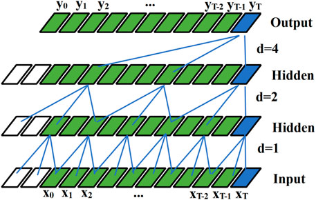
FIGURE 2. Expansion causal convolution.

2.2 CEEDMEAN algorithm

Empirical mode decomposition (EMD) is a means of smoothing non-stationary signals by converting a signal sequence into multiple intrinsic mode functions (IMFs) and residuals. EMD has been widely used in various fields but it still involves the problems of the mode aliasing phenomenon and end effect (Zhang et al., 2019b). These problems can be effectively suppressed by CEEMD.

The specific operation steps are as follows: first, the original signal x(t) to be decomposed is added to K times of Gaussian white noise with an average value of 0, and k times of sequences to be decomposed are constructed, i=1,2,3 $\dots$ k.

$x_i\left(t\right)=x\left(t\right)+\epsilon {\delta }_i\left(t\right)(2)$

Where $\epsilon$ is the weight coefficient of Gaussian white noise; ${\delta }_i\left(t\right)$ is the Gaussian white noise generated during the ith processing.

Then, decompose the empirical mode $x_i\left(t\right)$ and take the mean value of the first modal component obtained as the first modal component obtained $\text{IM}{\mathrm{F}}_1\left(\mathrm{t}\right)$ by CEEMDAN decomposition. Subsequently, obtain the margin signal of the first decomposition $\text{IM}{\mathrm{F}}_1\left(\mathrm{t}\right)$.

$IM{F}_1\left(t\right)=\frac{1}{K}{\displaystyle \sum _{i=1}^K}IM{F}_1^i\left(t\right)(3)$

$r_1\left(t\right)=x\left(t\right)-IM{F}_1\left(t\right)(4)$

Add specific noise to the margin signal at the jth stage and continue the EMD.

$IM{F}_j\left(t\right)=\frac{1}{K}{\displaystyle \sum _{i=1}^K}IM{F}_1^i\left(t\right)(5)$

$r_1\left(t\right)=x\left(t\right)-IM{F}_1\left(t\right)(6)$

Finally, if the EMD stops, the iteration stops and the CEEMDAN decomposition ends.

In this paper, CEEMDAN is mainly used to decompose the wind speed fluctuation segment, thereby reducing the complexity of the data, stabilizing the data, and preparing for the subsequent TCN-ATTENTION prediction.

2.3 Combined model of TCN-LSTM-CEEMDAN-ATTENTION

The TCN-LSTM-CEEMDAN-ATTENTION model (Figure 3) was established to predict the wind speed. As mentioned earlier, the wind speed data included the stationary and non-stationary segments. The LSTM model optimized by TCN has a strong ability to analyze and predict the data of the stationary segment. Furthermore, the TCN model after CEEMDAN decomposition and the subsequent addition of the attention mechanism has good performance for the separate prediction of the non-stationary segment.

FIGURE 3

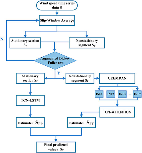
FIGURE 3. Forecast model flowchart.

Assuming the wind speed time series data S, firstly, the sliding window averaging method is used to distinguish the stationary segment S_P and the non-stationary segment S_F, and secondly, the TCN-LSTM model is used to predict the stationary segment S_P to obtain S_PP. Thereafter, the non-stationary segment S_F is decomposed by CEEMDAN to get INF={infi,i=1,2, $\dots$,7}. Then, each part of INF is predicted using TCN-ATTENTION to obtain S_FF. Finally, the two parts are combined and merged to obtain the final prediction result of the target sequence data ${\mathrm{S}}_Y={\mathrm{S}}_{PP}+{\mathrm{S}}_{FF}$.

The stationary segment S_P is an input sequence of length, where represents the input of the th time step. The first layer convolution operation of the TCN model can be expressed as:

${\mathrm{z}}_{\mathrm{t}}^{\left(\mathrm{l}\right)}=\mathrm{\varphi }\left({\mathrm{W}}^{\left(\mathrm{l}\right){\mathrm{x}}_{\mathrm{t}}^{\left(\mathrm{l}\right)}}+{\mathrm{b}}^{\left(\mathrm{l}\right)}\right)(7)$

Where $x^{\left(l\right)}t=\left[ht-k^{\left(l\right)}+1,h_{t-k^{\left(l\right)}+2},\dots ,h_t\right]$ represents the output vector of the current time step $t$ and its previous time step $k^{\left(l\right)}-1$, $W^{\left(l\right)}\in R^{F^{\left(l\right)}\times k^{\left(l\right)}}$ is a convolution kernel, $b^{\left(l\right)}\in R^{F^{\left(l\right)}}$ is a bias vector, and $\mathrm{\varphi }$ is a nonlinear activation function, usually ReLU. $z_t^{\left(l\right)}\in R^{F^{\left(l\right)}}$ represents the output vector of the convolutional operation of layer.

The layer $l$ convolution operation of the TCN model can be concatenated to form the output vector $z_t$ of the entire TCN model:

$z_t=\left[z_t^{\left(1\right)},z_t^{\left(2\right)},\dots ,z_t^{\left(L\right)}\right](8)$

Where L is the number of layers in the TCN model, 1 represents the output vector of the TCN model.

The hidden state vector of the LSTM model $h_t$ can be expressed as:

$i_t=\mathrm{\sigma }\left(W_{i{x}_t}+U_{i{h}_{t-1}}+b_i\right)(9)$

$f_t=\mathrm{\sigma }\left(W_{f{x}_t}+U_{f{h}_{t-1}}+b_f\right)(10)$

$o_t=\mathrm{\sigma }\left(W_{o{x}_t}+U_{o{h}_{t-1}}+b_o\right)(11)$

$\stackrel{\sim }{c_t}=\tanh \left(W_{c{x}_t}+U_{c{h}_{t-1}}+b_c\right)(12)$

${\mathrm{c}}_{\mathrm{t}}={\mathrm{f}}_{\mathrm{t}}\odot {\mathrm{c}}_{\mathrm{t}-1}+{\mathrm{i}}_{\mathrm{t}}\odot \stackrel{\sim }{{\mathrm{c}}_{\mathrm{t}}}(13)$

${\mathrm{h}}_{\mathrm{t}}={\mathrm{o}}_{\mathrm{t}}\odot \tanh \left({\mathrm{c}}_{\mathrm{t}}\right)(14)$

Here, ${\mathbf{i}}_{\mathbf{t}}$, ${\mathbf{f}}_{\mathbf{t}}$, and ${\mathbf{o}}_{\mathbf{t}}$ respectively represent the activation vectors of the input gate, forget gate, and output gate; $\stackrel{\sim }{{\mathbf{c}}_t}$ represents the candidate cell state vector at the current moment; ${\mathbf{c}}_{\mathbf{t}}$ represents the cell state vector at the current moment; and ${\mathbf{h}}_{\mathbf{t}}$ represents the hidden state vector at the current moment. ${\mathbf{W}}_{\mathbf{i}},{\mathbf{W}}_{\mathbf{f}},{\mathbf{W}}_{\mathbf{o}},{\mathbf{W}}_{\mathbf{c}}$ is the weight matrix of the input gate, forget gate, output gate and candidate cell states, ${\mathbf{U}}_{\mathbf{i}},{\mathbf{U}}_{\mathbf{f}},{\mathbf{U}}_{\mathbf{o}},{\mathbf{U}}_{\mathbf{c}}$ is the weight matrix of the corresponding hidden state, and ${\mathbf{b}}_{\mathbf{i}},{\mathbf{b}}_{\mathbf{f}},{\mathbf{b}}_{\mathbf{o}},{\mathbf{b}}_{\mathbf{c}}$ is the bias vector. $\sigma$ represents the sigmoid function, and $\odot$ represents element-wise multiplication.

The non-stationary segment S_F is decomposed into several IMFs using formula (15).

$\mathrm{s}\left(t\right)={\displaystyle \sum _{i=1}^n}{c}_i\left(t\right)+r_n\left(t\right)(15)$

where $s\left(t\right)$ is the non-stationary segment sequence S_F, $c_i\left(t\right)$ is the ith IMF, $r_n\left(t\right)$ is the remaining item, and $n$ is the number of IMFs.

Then, TCN is applied, that is, formulas (16–18) are applied to better capture long-term dependencies.

$y=f\left(x\right)+g\left(x\right)(16)$

$f\left(x\right)=\mathrm{\sigma }\left(W_{1}x+b_1\right)(17)$

$g\left(x\right)=\mathrm{\sigma }\left(W_2\left(\mathrm{\delta }\left(x\right)*x\right)+b_2\right)(18)$

where, $x$ is the input sequence, $y$ is the output sequence, $\sigma$ is the Activation function, $W_1,W_2$ is the weight matrix, $b_1,b_2$ is the bias vector, $*$ represents convolution operation, $\delta \left(x\right)$ is an extensible Dilated Revolution operation。

Finally, by combining CEEMDAN and TCN, and adding the Attention mechanism, the CEEMDAN-TCNN Attention model (Formula 19) is obtained:

$h_t={\displaystyle \sum _{i=1}^n}{\alpha }_i\bullet T^N\left(C^N\left(x_{1:T}\right)\right)\left[i,t\right](19)$

Where, ${\mathit{h}}_{\mathit{t}}$ is the output of the first time step, $C^N$ is a CEEMDAN operation, $T^N$ is TCN operation, ${\alpha }_i$ is the Attention weight.

3 Experimental process

3.1 Data sources

The data was collected from a mining site in western China,specifically an open-pit mining area, spanning from September 13 to 17, 2022, totaling 5 days. A set of 7,200 data points was gathered, each spaced at 1-min intervals, There are six parameters in the data set (Table 1), serving as the focus of our research (see Figure 4). As depicted in the figure, it is evident that the wind speed data exhibits irregular and unstable patterns.

FIGURE 4

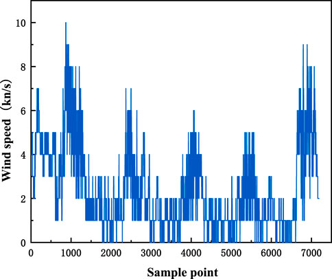
FIGURE 4. Raw wind speed time series.

TABLE 1

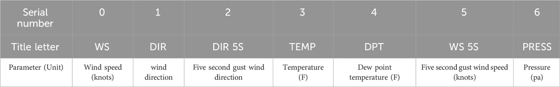
TABLE 1. Data parameters.

3.2 Data stationarity and non-stationarity division

In this study, 7,200 sets of data were used, of which 5,760 were used as the training sequence set of the overall model and the remaining 1,440 were used as the test sequence set to test and verify the generalization ability of the model. First, the shadow matrix method of the original data set was used to assess the lack of data in the data set. The shadow matrix is a copy of the weight matrix, and its value is updated by the main weight matrix. Moreover, its historical information is maintained to a certain extent. If the value of the shadow matrix element is 1, the corresponding position value of the original dataset is a missing state; otherwise, if the value of the shadow matrix element is 0, the corresponding value in the original data set exists. A description of the statistics of missing raw data is provided in Table 2. Considering the low proportion of missing data, the impact of missing data on the integrity of the model is small, and deleting missing data will not cause data deviation. Accordingly, the direct deletion method was used for data preprocessing.

TABLE 2

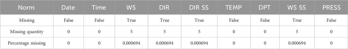
TABLE 2. Missing data situation.

After data preprocessing, the data were resampled at 1-h intervals in order to rapidly and intuitively extract information on the structural kernel properties of the data in the population distribution (Li et al., 2016). Figure 5A presents a graph of the time-varying sum of resampled wind speed for 1 hour, and Figure 5B presents a graph of the time-varying graph of the resampled average value of wind speed for 1 hour. According to the change graph, the average value and sum of the resampled data set have a similar structure, and the overall volatility has certain rules. To improve the accuracy of the data analysis, the original wind speed data and the 1-h, 5-h, and 7-h re-sampling data were tested for correlation. As shown in Figure 6, with increasing the sampling time, the correlation between the wind direction and the 5-s gust wind direction first increases and then decreases, and the correlation characteristics between other variables become more prominent. The reason is that when the resampling interval increases from a smaller value, the correlation will increase because the relationship between data points becomes clearer and more salient. However, after reaching a certain resampling interval, the variation between data points becomes irregular and chaotic, weakening the correlations. This is because the interactions between data points become more difficult to capture and analyze. Therefore, the relationship between resampling interval and correlation usually presents a curve of initial rise followed by a fall.

FIGURE 5

FIGURE 5. Hourly resampling of wind speed. (A): Hourly resampling sum of wind speed over time, (B): Hourly resampled mean wind speed over time.

FIGURE 6

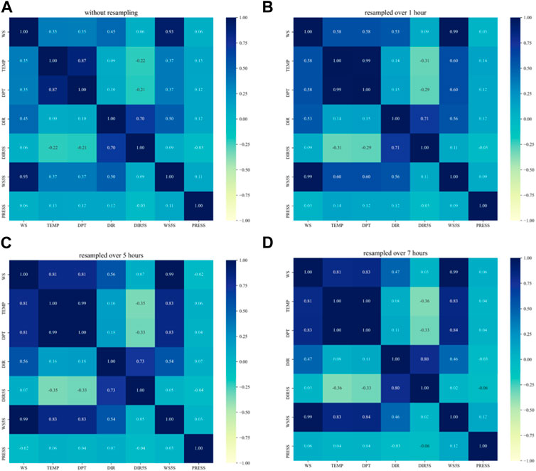
FIGURE 6. Data correlation test. (A): Correlation of variables in raw data, (B): Correlation of variables after 1-h resampling, (C): Correlation of variables after 5-h resampling, (D): Correlation of variables after 7-h resampling.

In the heat map, the correlation trend of wind speed and wind direction, and the wind direction of the 5-s gust all increase first and then decrease, with the highest values of 0.56 and 0.09 respectively. The overall correlation is low. However, the temperature and dew point temperature do not exhibit any downward trend with increasing sampling time. As a result, their correlation is more prominent in the 7-h resampling. For the 7-h interval, the top three variables most correlated with wind speed are 5-s gust wind speed (correlation parameter 1.00), dew point temperature (correlation parameter 0.83), and air temperature (correlation parameter 0.81). As the 5-s gust wind speed was obtained from wind speed data, it is not a factor affecting the wind speed sequence. Moreover, as the dew point temperature was calculated from air temperature, humidity, and atmospheric pressure, the reflected data characteristics are more comprehensive. Therefore, the dew point temperature was selected as the largest variable affecting the wind speed. Figure 7 presents a sequence diagram of wind speed and dew point temperature. As shown in the figure, when the dew point temperature is a trough, the wind speed sequence is a stationary segment. The larger the trough span, the longer the duration of the stationary segment of the wind speed sequence.

FIGURE 7

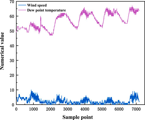
FIGURE 7. Sequence diagram of wind speed and dew point temperature.

The preprocessed data were divided using the sliding window average method in the threshold method. First, the time series data were divided into fixed-size sliding windows, and then for each window, the average value of all data in the window was calculated. Using the average value as the representative value of the window, the window was slid forward by one unit, and the average value was continuously calculated until the window slid to the end of the sequence. The optimal threshold range was determined using the grid search method, which is a hyperparameter tuning method for automatically selecting the optimal parameters in the model. It evaluates and compares all possible hyperparameter combinations to find the optimal hyperparameter combination by performing an exhaustive search on a specified parameter grid. The sliding window average method in the threshold method is used to segment the preprocessed data. The time series data is first divided into fixed-size sliding Windows, and then the average of all the data within the window is calculated for each window. Using the mean as the representative value of the window, slide the window forward one unit and continuously calculate the mean until the window slides to the end of the sequence. The optimal threshold range is determined by the grid search method, which is a hyperparameter tuning method that automatically selects the optimal parameters in the model. It evaluates and compares all possible hyperparameter combinations, and finds the optimal hyperparameter combination through exhaustive search of the specified parameter grid. The MyModel class calculates the mean and variance in the time series data. It then traverses the data points to find the first point that breaks the threshold, marking it as non-stationary. This non-stationary point is used to cut the time series data. The program creates a Pipeline with the MyModel class as one of the steps. Define the param_grid parameter, which includes a range of different thresholds. GridSearchCV was used for grid search, and the model performance under different thresholds was evaluated through cross-validation, with MSE as the evaluation index. Finally, the threshold with the best performance was found, the optimal threshold was set to 2.2 (Table 3), and the sliding window average method was used to obtain the time nodes of the stationarity and non-stationarity of the wind speed series on the training day (Table 4). In order to ensure reasonable data segmentation, the average value of time node 15:17 is taken as the segmentation point.

TABLE 3

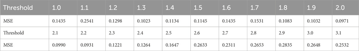
TABLE 3. Threshold selection.

TABLE 4

TABLE 4. Smooth sequence delineation of timing nodes.

After dividing the data, the unit root (Augmented Dickey-Fuller test, ADF) test was used to conduct time series division test, and the stability of the data was assessed according to the occurrence of ADF in the time series. The presence of ADF indicates unstable data and vice versa. In the ADF test, the p-value is evaluated against the 0.05 confidence interval. If the p-value is less than 0.05, it can be considered that the null hypothesis is rejected, the data does not have a unit root, and the sequence is stable; if it is greater than or equal to 0.05, the null hypothesis cannot be significantly rejected. In this case, further significant test statistics are required. If the significant test statistic is less than three confidence levels (10%, 5%, 1%), then there is (90%, 95, 99%) certainty to reject the null hypothesis, otherwise the data are considered to be non-stationary. The stationary and non-stationary sequences were extracted from the divided training set (Figure 8).

FIGURE 8

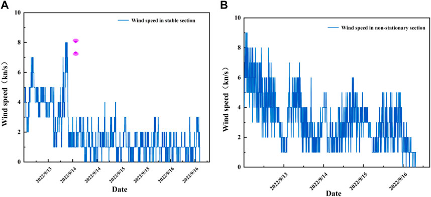
FIGURE 8. Stability division of wind speed training data. (A): Smooth sequence segment of training data, (B)Training data non-stationary sequence segments.

The ADF test results of the extracted data are shown in Table 5. The T value of the first sequence was -4.2045 and less than 1%, 5%, and 10%, indicating rejection of the hypothesis. Moreover, the p-value of 0.00064 is significant at 5%, verifying the rejection of the null hypothesis, and thus the stationarity of the data. The T value of the second sequence was -3.0680, and it was not less than 1%, 5%, and 10% at the same time, indicating that the hypothesis cannot be rejected, and that the data is non-stationary. These results proved that partitioning of the data according to stationarity was successful.

TABLE 5

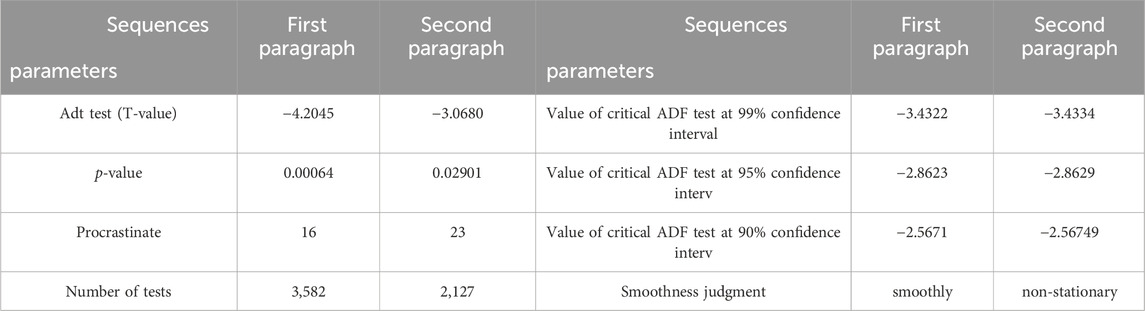
TABLE 5. Using ADF test to partition data.

3.3 Wind speed prediction and fitting effect

Through the division of data described in the previous section, the stationary and non-stationary data sequences were successfully obtained. Next, TCN-LSTM was used to process the stationary data, and CEEMDAN-TCN-ATTENTION was used to process the non-stationary data.

3.3.1 TCN-LSTM model prediction

Before model training, the wind speed and dew point temperature in the stationary segment and the non-stationary segment sequence were aligned according to the time axis, and the wind speed and dew point temperature at each time point were used as multivariate data at that time point, thereby obtaining a multivariate time series. The model was trained using this multivariate time series.

The TCN-LSTM model was trained with 3,600 sets of data and used to predict the stationary part of the wind speed time series. The sample sequence was converted into a supervised learning sequence and then normalized. The model first defines the TCN model. Then, the parameters are optimized using the following evaluation indicators: mean absolute error (MAE), mean squared error (MSE), root mean squared error (RMSE) and R squared error (R2).

The initial parameters were set as follows: loss function MSE, filters=2, Kernel_size=2, Dropout=0.23, Epochs=4,000.

(1) Filter optimization

Filters refer to the number of convolution kernels used in the convolution layer, and each convolution kernel can extract a specific feature. Therefore, the size of filters affects the number and complexity of features learned by the model. With Kernel_size=3, Dropout=0.2, and Epochs=2000, the test sets were compared among Filters of 2, 3, and 4.

As shown in Figure 9 (a) and Table 6, MAE, MSE, RMSE, and R² did not exhibit large numerical changes with increasing values of filters. The reason is that the feature space of the input data set is not very complicated, and the use of more filters will not bring significant improvements. In order to obtain more accurate predictions, the filter value was set at 3.

(2) Kernel_size optimization

FIGURE 9

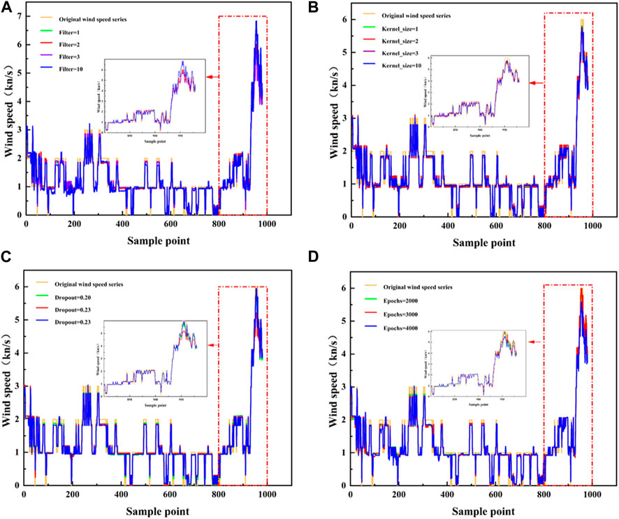
FIGURE 9. TCN-LSTM model tuning. (A) Comparison of predictions of different Filter value models, (B) Comparison of model predictions for different Kernel_size values, (C) Comparison of model predictions for different Dropout values, (D) Comparison of model predictions for different Epochs values.

TABLE 6

TABLE 6. TCN-LSTM model parameter adjustment evaluation form.

With Filters=3, Dropout=0.2, and Epochs=2000, the test sets were compared among Kernel_sizes of 1, 2, and 3.

Kernel_size refers to the size of the convolution kernel, which is usually a square or rectangular matrix. The convolution kernel slides and extracts features during the convolution process. Kernel_size will affect the size and shape of the features learned by the model. A larger Kernel_size can usually capture a wider range of features, but it will increase the amount of calculation and the complexity. As shown in Figure 9 (b) and Table 6, the increase in the value of Kernel_size did not cause much change. The reason is that the features in the data set are small, and more useful features cannot be learnt by increasing Kernel_size. To improve the prediction accuracy, the Kernel_size was set at 1.

(3) Dropout optimization

With Filters=3, Kernel_size=10, and Epochs=2000, the test sets were compared among Dropouts of 0.20, 0.23, and 0.26.

As shown in Figure 9 (c), and Table 6, the best results were obtained at Dropout=0.26, with MAE=0.1853 knots, MSE=0.0953 knots², RMSE=0.3087 knots, and R2=0.9108.

(4) Epoch optimization

With Filters=3, Kernel_size=10, and Dropout=0.26, the test sets were compared among Epochs of 2000, 3,000 and 4,000.

As shown in Figure 9 (d), and Table 6, the best results were obtained at Epochs=2000, with MAE=0.1913 knots, MSE=0.0953 knots², RMSE=0.3087 knots, and R2=0.9108.

Considering these results, the main parameters of the TCN-LSTM wind speed plateau sequence model were set as follows: Filters=3, Kernel_size=10, Dropout=0.26, and Epochs=2000. The comparison between the prediction and actual situation is shown in Figure 10.

FIGURE 10

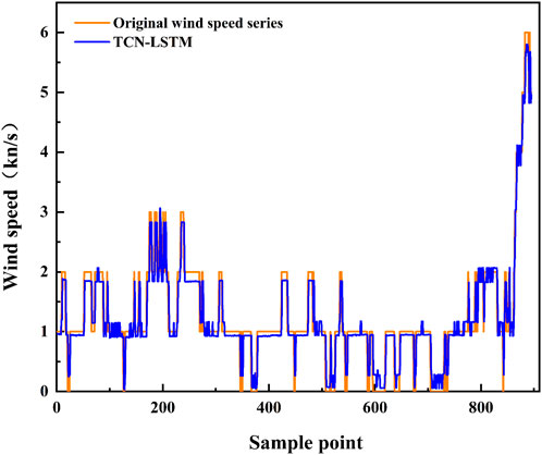
FIGURE 10. Prediction of stationary wind speed data using TCN-LSTM model.

3.3.2 CEEMDAN-TCN-ATTENTION model prediction

The CEEMDAN-TCN-ATTENTION model was used to predict the non-stationary segment of the wind speed time series, and 2,160 sets of data were used for training. As shown in Figure 11, CEEMDAN divided the wind speed data were divided into modal components (IMF1–IMF7) and residual sequence (Res), arranged in order of frequency from high to low. In CEEMDAN, each IMF is obtained by extracting and interpolating a series of local mean and extreme points from the original data. Each IMF represents a specific vibrational mode in the data, with distinct time-scale and frequency signatures. Residual series are leftover data, usually considered noise or random disturbances. As shown in Figure 11, IMF1 usually represents high-frequency noise or the trend of high-frequency changes, and may have negligible relationship with independent variables, but IMF2 to IMF7 represent lower and lower frequency components, and the change patterns of these IMFs can reflect each independent variable. Therefore, IMF2 to IMF7 respectively represent the influence of sknt(wind speed), drct(wind direction), gust_drct(5-s gust wind direction), Tmpf,(temperature) Dwpf(dewpoint temperature), gust_sknt(5-s gust wind speed), and pres1(pressure) on wind speed. IMF5 and the original data exhibit the same trend.

FIGURE 11

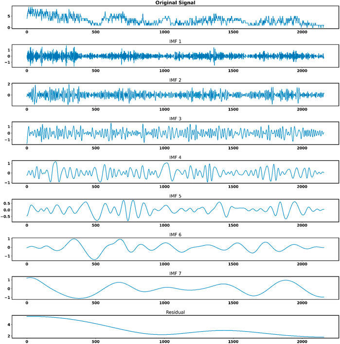
FIGURE 11. CEEMDAN decomposition diagram.

Combined with the correlation analysis in Figure 6, the dew point temperature was verified to be the main influencing factor of wind speed, with a positive correlation between them. The TCN-ATTENTION model was then run for each IMF separately.

The model first defines the TCN model, then adds the self-attention layer, and then optimizes related parameters. The following evaluation indicators were used: MAE, MSE, RMSE, and R2.

(1) Unit optimization

In self-attention, the unit parameter is usually used to specify the vector dimension of the input sequence. First, the basic parameters in the combined model were set. In actual use, the size of units can be adjusted according to the application scenario and the complexity of the model. A larger value of units may increase the representation ability of the model, but it will also increase the calculation time and training complexity of the model. The initial parameters were set as follows: loss function MSE, Dropout=0.3, Filters=5, Kernel_size=2, Epochs=300. The performance of the test set was compared with unit sizes of 10,000, 20,000, and 30,000.

As shown in Figure 12A and Table 7, the best performance was achieved at the unit size of 20,000, with MAE, MSE, RMSE, and R2 of 0.1602 knots, 0.0340 knots ², 0.1844 knots, and 0.9879, respectively.

(2) Dropout optimization

FIGURE 12

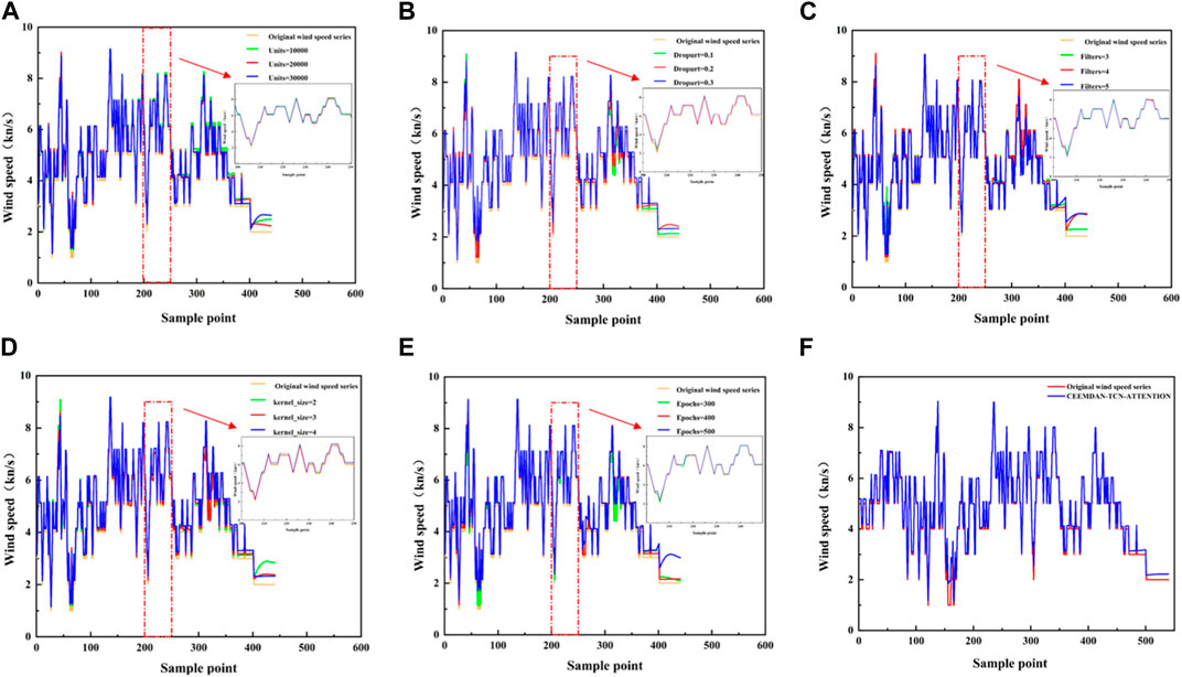
FIGURE 12. CEEMDAN-TCN-ATTENTION model tuning. (A) Comparison of model predictions for different Units values, (B) Comparison of model predictions for different Dropurt values, (C) Comparison of model predictions for different Filters values, (D) Comparison of model predictions for different Kernel_size values, (E) Comparison of model predictions for different Epochs values, (F) Prediction of non-stationary wind speed data.

TABLE 7

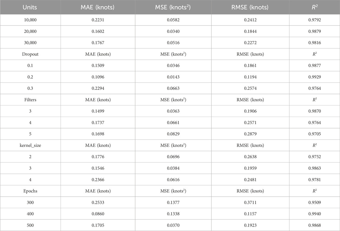
TABLE 7. CEEMDAN-TCN-ATTENTION model parameter adjustment evaluation form.

With Units=20,000, Filters=5, Kernel_size=2, and Epochs=300, the test sets with Dropout of 0.1, 0.2, and 0.3 were compared.

As shown in Figure 12Band Table 7, the best performance was achieved at the dropout of 0.2, with MAE, MSE, RMSE, and R2 of 0.1096 knots, 0.0143 knots², 0.1194 knots, and 0.9949, respectively.

(3) Filter optimization

With Units=20,000, Dropout=0.2, Kernel_size=2, and Epochs=300, the test sets were compared among Filters of 3, 4, and 5.

As shown in Figure 12C and Table 7, the best performance was achieved at the Filter value of 3, with MAE, MSE, RMSE, and R2 of 0.1499 knots, 0.0363 knots², 0.1906 knots, and 0.9870, respectively.

(4) Kernel_size optimization

With Units=20,000, Dropout=0.2, Filters=4, and Epochs=300, the test sets were compared among Kernel_size of 2, 3 and 4.

As shown in Figure 12D and Table 7, the best performance was achieved at the Kernel_size of 3, with MAE, MSE, RMSE, and R2 of 0.1546 knots, 0.0384 knots², 0.1959 knots, and 0.9863, respectively.

(5) Epoch optimization

The same method was used to optimize the Epochs parameter. With Units=20,000, Dropout=0.2, Filters=4, and Kernel_size=1, the test sets were compared among Epochs of 300, 400, and 500.

As shown in Figure 12E and Table 7, the CEEMDAN-TCN-ATTENTION model showed the best performance for the non-stationary segment at the Epoch value of 400, with MAE, MSE, RMSE, and R2 of 0.0860 knots, 0.1338 knots², 0.1157 knots, and 0.9950, respectively. The prediction graph is shown in Figure 12F.

3.3.3 Combined model of TCN-LSTM-CEEMDAN-ATTENTION

A total of 18,800 sets of data from a wind farm in western China September 13 to 16, 2022 were used to train the combined model. TCN-LSTM was used to predict stationary sequences, and CEEMDAN-TCN-ATTENTION was used to predict non-stationary sequences. Finally, the TCN-LSTM -CEEMDAN-ATTENTION combined model was used to predict 1,440 sets of data on September 17. The main parameters of the TCN-LSTM model for the stationary segment were set as follows: Filters=3, Kernel_size=10, Dropout=0.26, and Epochs=2000. The main parameters of the CEEMDAN-LSTM-ATTENTION model for the non-stationary segment sequence were set as follows: Units=20,000, Dropout=0.2, Filters=4, Kernel_size=1, and Epochs=400. The overall prediction plot of the model is shown in Figure 13.

FIGURE 13

FIGURE 13. Overall model wind speed data prediction.

4 Discussion

The TCN-LSTM-CEEMDAN-ATTENTION model was compared with the TCN-LSTM-VMD-ATTENTION and TCN-LSTM-EMD-ATTENTION models. Figures 14A,B show prediction comparison charts of the TCN-LSTM-CEEMDAN-ATTENTION model with the TCN-LSTM-VMD-ATTENTION and TCN-LSTM-EMD-ATTENTION models, respectively. Figure 14C presents a comparison diagram of the three different decomposition algorithms. Table 8 lists the evaluation indicators of the three different decomposition algorithms. As shown in Figures 14, 15 and Table 8, the overall MAE, MSE, and RMSE of the model with CEEMDAN are better than those with the other two algorithms. The model predicted data and the actual value fit well. These results prove that the use of CEEMDAN in the decomposition process of this model is optimal.

FIGURE 14

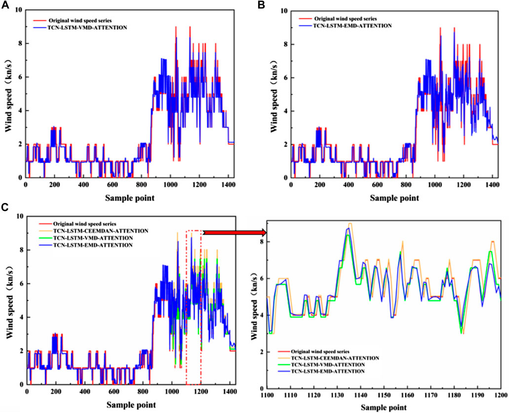
FIGURE 14. Comparison of the prediction results of each decomposition model. (A) TCN-LSTM-VMD-ATTENTION Forecast Comparison Chart, (B) TCN-LSTM-EMD-ATTENTION Forecast Comparison Chart. (C) Comparison of prediction results of different decomposition models.

TABLE 8

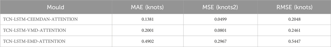
TABLE 8. Analysis of prediction results of different decomposition models.

FIGURE 15

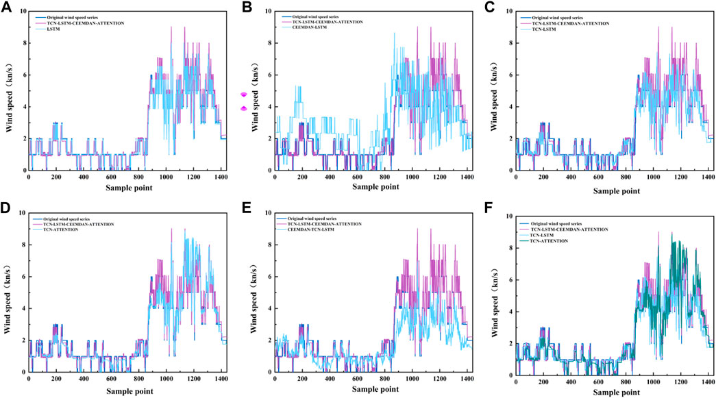
FIGURE 15. Comparison of the results of the predictions of the models. (A) Comparison between the model and LSTM prediction in this article, (B) Comparison between the model and CEEMDAN-LSTM prediction in this article, (C) Comparison between the model and TCN-LSTM prediction in this article, (D) Comparison between the model and TCN-ATTENTION in this article, (E) Comparison between the model and CEEMDAN-TCN-LSTM prediction in this article, (F) Comparison between the model in this article and some models’ predictions.

The TCN-LSTM-CEEMDAN-ATTENTION model was compared with the LSTM model alone, CEEMDAN-LSTM model, TCN-LSTM model, TCN-ATTENTION model, and CEEMDAN-TCN-ATTENTION model. A comparison chart is shown in Figure 15. In order to evaluate the prediction accuracy of each model more accurately, three indicators were used: MAE, MSE, and RMSE. The prediction results of each model are listed in Table 9.

TABLE 9

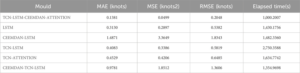
TABLE 9. Comparison of prediction results of different models.

Table 9 shows that the MAE, MSE, and RMSE of the TCN-LSTM-CEEMDAN-ATTENTION model are the smallest at 0.1381 knots, 0.0499 knots², and 0.2048 knots, respectively. Accordingly, it can be concluded that the TCN-LSTM-CEEMDAN-ATTENTION model has superior prediction performance, and is thus more suitable for ultra-short-term wind speed prediction.

In this experiment, the time consumed by each model (TCN-LSTM-CEEMDAN-ATTENTION, LSTM, CEEMDAN-LSTM, TCN-LSTM, TCN-ATTENTION, and CEEMDAN-TCN-ATTENTION) throughout the run was recorded. As shown in Table 9, the overall runtime of the TCN-LSTM-CEEMDAN-ATTENTION model is smaller than that of the other models. Therefore, it can be concluded that the efficiency of the TCN-LSTM and CEEMDAN-TCN-ATTENTION processes improve after the data are divided by stationarity.

We also compared the evaluation parameters of the ultra short term wind speed prediction models established by other researchers, including Yan et al.'s article “Wind speed prediction using a hybrid model of EEMD and LSTM considering seasonal features” (Yan et al., 2022), Zhang et al.'s article“A comprehensive wind speed prediction system based on Monte Carlo and artificial intelligence algorithms” (Zhang et al., 2022b), Wang et al.'s article “Wind speed prediction using measurements from neighboring locations and combining the extreme learning machine and the AdaBoost algorithm” (Wang et al., 2022), Ji et al.'s article “Short-Term Canyon Wind Speed Prediction Based on CNN—GRU Transfer Learning” (Ji et al., 2022). The comparative data is shown in Table 10. After comparing models in similar articles, the model established in this article still has significant advantages and is suitable for ultra short term wind speed prediction.

TABLE 10

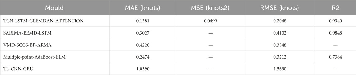
TABLE 10. Comparison of models in similar types of articles.

5 Conclusion

This study introduces and validates a state-of-the-art real-time prediction model for ultra-short-term wind speeds using a dual-model framework consisting of the TCN-LSTM and CEEMDAN-TCN-ATTENTION architectures. The main objective of this study is to improve the efficiency of geotechnical hazard monitoring and early warning systems, with a special focus on open pit mining areas. The excellent predictive accuracy and efficiency of the model in predicting ultra-short-term wind speeds highlights its key role in advancing smart geotechnical hazard monitoring.

A noteworthy contribution of this investigation lies in its methodical treatment of the distinctive characteristics inherent in stationary and non-stationary sequences within ultra-short-term wind speed time series. The application of the sliding window averaging method facilitated the categorization of wind speed series into stationary and non-stationary components. The TCN-LSTM model demonstrated proficiency in predicting the stationary sequence, leveraging its dilated causal convolution and LSTM units for discerning time correlations and maintaining temporal continuity. Concurrently, for the non-stationary sequence, the CEEMDAN-TCN-ATTENTION model, incorporating CEEMDAN for data simplification and ATTENTION for enhanced TCN data capture, proved effective. The amalgamation of these models yielded the robust TCN-LSTM-CEEMDAN-ATTENTION model.

The comparative analysis involving various decomposition algorithms and five distinct single and combined models accentuated the superior predictive capabilities of our proposed integrated model. With minimal Mean Absolute Error (MAE) of 0.1381, Mean Squared Error (MSE) of 0.0499, and Root Mean Squared Error (RMSE) of 0.2048, our model surpassed alternative approaches. Its prediction fit outperformed other models, reinforcing its suitability for ultra-short-term wind speed prediction.

The model is important for geotechnical hazard monitoring, especially in open pit mining areas. The validated model not only improves our understanding of ultrashort-term wind speed dynamics, but also provides a practical and efficient tool for real-time prediction. The success of our approach highlights its potential for wider application in geotechnical monitoring systems, promising improved safety and operational efficiency in high-risk environments. Integrating this advanced predictive model into an operating system is a key step towards a more resilient and responsive approach to geotechnical disaster management.

Data availability statement

The datasets presented in this study can be found in online repositories. The names of the repository/repositories and accession number(s) can be found below: https://mesonet.agron.iastate.edu/COOP/extremes.php.

Author contributions

PS: Writing–original draft, Writing–review and editing. JW: Writing–review and editing, Supervision. ZY: Writing–review and editing.

Funding

The author(s) declare that financial support was received for the research, authorship, and/or publication of this article. This work was supported by Shaanxi Province key industrial chain project (2023-ZDLGY-24).

Acknowledgments

We are very grateful for the support of Shaanxi Nano Research Laboratory and Shaanxi Province (2023-ZDLGY-24) for this project. We also appreciate the feedback from reviewers, which has been very helpful in improving the manuscript.

Conflict of interest

The authors declare that the research was conducted in the absence of any commercial or financial relationships that could be construed as a potential conflict of interest.

Publisher’s note

All claims expressed in this article are solely those of the authors and do not necessarily represent those of their affiliated organizations, or those of the publisher, the editors and the reviewers. Any product that may be evaluated in this article, or claim that may be made by its manufacturer, is not guaranteed or endorsed by the publisher.

Abbreviations

TCN, Temporal Convolutional Network; ADF, Augmented Dickey-Fuller; LSTM, Long Short Term Memory; CEEMDAN, Complete Ensemble Empirical Mode Decomposition with Adaptive Noise; GPR, Gaussian Process Regression; GA, Genetic Algorithm; ANN, Artificial Neural Network; VMD, Variational Mode Decomposition; NWP, Numerical Weather Prediction; MOS, Mos Forecasting Method; WRF, Weather Research and Forecasting Model; NWP, Numerical Weather Prediction; ARIMA, Autoregressive Integrated Moving Average Model; SVM, SupportVectorMachine; ANN, Artificial Neural Network; MLP, Multilayer Perceptron; SAM, Segment Anything Model; RBFN, Radial basis function network; GWO, Grey Wolf Optimization; GRU, Gate Recurrent Unit.

References

Al-Yahyai, S., Charabi, Y., Gastli, A. J. R., and Reviews, S. E. (2010). Review of the use of numerical weather prediction (NWP) models for wind energy assessment. Renew. Sustain. Energy Rev. 14, 3192–3198. doi:10.1016/j.rser.2010.07.001

CrossRef Full Text | Google Scholar

Chandra, D. R., Kumari, M. S., and Sydulu, M. (2013). “A detailed literature review on wind forecasting,” in Proceedings of the 2013 International Conference on Power, Energy and Control (ICPEC), Dindigul, India, February 2013 (IEEE), 630–634.

CrossRef Full Text | Google Scholar

Chen, X., Li, L., Wang, L., and Qi, L. (2019). The current situation and prevention and control countermeasures for typical dynamic disasters in kilometer-deep mines in China. Saf. Sci. 115, 229–236. doi:10.1016/j.ssci.2019.02.010

CrossRef Full Text | Google Scholar

Cheng, W. Y., Liu, Y., Liu, Y., Zhang, Y., Mahoney, W. P., and Warner, T. T. (2013). The impact of model physics on numerical wind forecasts. Renew. Energy 55, 347–356. doi:10.1016/j.renene.2012.12.041

CrossRef Full Text | Google Scholar

Erdem, E., and Shi, J. (2011). ARMA based approaches for forecasting the tuple of wind speed and direction. Appl. Energy 88, 1405–1414. doi:10.1016/j.apenergy.2010.10.031

CrossRef Full Text | Google Scholar

Fu, W., Wang, K., Li, C., and Tan, JJEC (2019). Multi-step short-term wind speed forecasting approach based on multi-scale dominant ingredient chaotic analysis, improved hybrid GWO-SCA optimization and ELM. Energy Convers. Manag. 187, 356–377. doi:10.1016/j.enconman.2019.02.086

CrossRef Full Text | Google Scholar

Giebel, G., Draxl, C., Brownsword, R., Kariniotakis, G., and Denhard, M. (2011). The state-of-the-art in short-term prediction of wind power. A lit. Overv. doi:10.13140/RG.2.1.2581.4485

CrossRef Full Text | Google Scholar

Hepbasli, A. J. R. (2008). A key review on exergetic analysis and assessment of renewable energy resources for a sustainable future. Renew. Sustain. Energy Rev. 12, 593–661. doi:10.1016/j.rser.2006.10.001

CrossRef Full Text | Google Scholar

Huang, N. E., Shen, Z., Long, S. R., Wu, M. C., Shih, H. H., Zheng, Q., et al. (1998). The empirical mode decomposition and the Hilbert spectrum for nonlinear and non-stationary time series analysis. Proc. R. Soc. Lond. A 454, 903–995. doi:10.1098/rspa.1998.0193

CrossRef Full Text | Google Scholar

Ji, L., Fu, C., Ju, Z., Shi, Y., Wu, S., and Tao, L. J. A. (2022). Short-Term canyon wind speed prediction based on CNN—GRU transfer learning. Atmos. (Basel). 13, 813. doi:10.3390/atmos13050813

CrossRef Full Text | Google Scholar

Kavasseri, R. G., and Seetharaman, K. J. (2009). Day-ahead wind speed forecasting using f-ARIMA models. Renew. Energy 34, 1388–1393. doi:10.1016/j.renene.2008.09.006

CrossRef Full Text | Google Scholar

Khazaei, S., Ehsan, M., Soleymani, S., and Mohammadnezhad-Shourkaei, H. J. E. (2022). A high-accuracy hybrid method for short-term wind power forecasting. Energy 238, 122020. doi:10.1016/j.energy.2021.122020

CrossRef Full Text | Google Scholar

Kulkarni, M. A., Patil, S., Rama, G., and Sen, P. J. (2008). Wind speed prediction using statistical regression and neural network. J. Earth Syst. Sci. 117, 457–463. doi:10.1007/s12040-008-0045-7

CrossRef Full Text | Google Scholar

Kunyan, Z., and Meihong, LJCMM (2019). Slope stability prediction of open-pit mine based on GA-BP model. CHINA Min. Mag. 28, 144–148. doi:10.12075/j.issn.1004-4051.2019.06.023

CrossRef Full Text | Google Scholar

Li, W., Qiao, S., Zhang, H., Zheng, Q., and Yang, S. (2022). “Ultra-short-term wind power forecasting model based on improved whale algorithm and LSTM neural network,” in Proceedings of the 4th International Conference on Information Science, Electrical, and Automation Engineering (ISEAE 2022), Beijing, China, September 2019 (SPIE), 153–159.

CrossRef Full Text | Google Scholar

Li, Y., Zhao, Y., Wang, L., Zhang, M., and Zhou, M. (2016). Variance estimation considering multistage sampling design in multistage complex sample analysis. Zhonghua liu xing bing xue za zhi = Zhonghua liuxingbingxue zazhi 37, 425–429. doi:10.3760/cma.j.issn.0254-6450.2016.03.028

PubMed Abstract | CrossRef Full Text | Google Scholar

Liu, H. P., Shi, J., and Erdem, E. (2013). An integrated wind power forecasting methodology: interval estimation of wind speed, operation probability of wind turbine, and conditional expected wind power output of A wind farm. Int. J. Green Energy 10, 151–176. doi:10.1080/15435075.2011.647170

CrossRef Full Text | Google Scholar

Liu, M.-D., Ding, L., and Bai, Y.-LJEC (2021). Application of hybrid model based on empirical mode decomposition, novel recurrent neural networks and the ARIMA to wind speed prediction. Energy Convers. Manag. 233, 113917. doi:10.1016/j.enconman.2021.113917

CrossRef Full Text | Google Scholar

Luo, H., Dou, X., Sun, R., and Wu, S. J. (2021a). A multi-step prediction method for wind power based on improved TCN to correct cumulative error. Front. Energy Res. 9, 723319. doi:10.3389/fenrg.2021.723319

CrossRef Full Text | Google Scholar

Luo, H. F., Dou, X., Sun, R., and Wu, S. J. (2021b). A multi-step prediction method for wind power based on improved TCN to correct cumulative error. Front. Energy Res. 9. doi:10.3389/fenrg.2021.723319

CrossRef Full Text | Google Scholar

Mohandes, M. A., Halawani, T. O., Rehman, S., and Hussain, A. A. (2004). Support vector machines for wind speed prediction. Renew. Energy 29, 939–947. doi:10.1016/j.renene.2003.11.009

CrossRef Full Text | Google Scholar

Mölders, N. J. M., and Physics, A. (1999). On the atmospheric response to urbanization and open-pit mining under various geostrophic wind conditions. Meteorol. Atmos. Phys. 71, 205–228. doi:10.1007/s007030050056

CrossRef Full Text | Google Scholar

Nie, L., Li, Z., Lv, Y., Wang, H. J., and Environment, t (2017). A new prediction model for rock slope failure time: a case study in West Open-Pit mine, Fushun, China. Bull. Eng. Geol. Environ. 76 (3), 975–988. doi:10.1007/s10064-016-0900-8

CrossRef Full Text | Google Scholar

Parra, E., Mohr, C. H., and Korup, OJGRL (2021). Predicting Patagonian landslides: roles of forest cover and wind speed. Geophys. Res. Lett. 48, e2021GL095224. doi:10.1029/2021gl095224

CrossRef Full Text | Google Scholar

Peng, X., and Lu, G. J. (1995). Physical modelling of natural wind and its guide in a large open pit mine. J. Wind Eng. Industrial Aerodynamics 54, 473–481. doi:10.1016/0167-6105(94)00060-q

CrossRef Full Text | Google Scholar

Ranganayaki, V., and Deepa, S. N. (2019). Linear and non-linear proximal support vector machine classifiers for wind speed prediction. Clust. Computing-the J. Netw. Softw. Tools Appl. 22, 379–390. doi:10.1007/s10586-018-2005-6

CrossRef Full Text | Google Scholar

Shobana Devi, A., Maragatham, G., Boopathi, K., Lavanya, M., and Saranya, R. (2020). “Long-term wind speed forecasting—a review,” in Proceedings of the Artificial Intelligence Techniques for Advanced Computing Applications, Singapore, July 2020 (Springer), 79–99.

CrossRef Full Text | Google Scholar

Ssekulima, E. B., Anwar, M. B., Al Hinai, A., and El Moursi, M. S. (2016). Wind speed and solar irradiance forecasting techniques for enhanced renewable energy integration with the grid: a review. IET Renew. Power Gener. 10, 885–989. doi:10.1049/iet-rpg.2015.0477

CrossRef Full Text | Google Scholar

Sun, W., Liu, M., and Liang, Y. J. E. (2015). Wind speed forecasting based on FEEMD and LSSVM optimized by the bat algorithm. Energies (Basel). 8, 6585–6607. doi:10.3390/en8076585

CrossRef Full Text | Google Scholar

Sun, W., and Wang, X. (2022). Improved chimpanzee algorithm based on CEEMDAN combination to optimize ELM short-term wind speed prediction. Environ. Sci. Pollut. Res. 30, 35115–35126. doi:10.1007/s11356-022-24586-1

PubMed Abstract | CrossRef Full Text | Google Scholar

Tascikaraoglu, A., Uzunoglu, M. J. R., and Reviews, S. E. (2014). A review of combined approaches for prediction of short-term wind speed and power. Renew. Sustain. Energy Rev. 34, 243–254. doi:10.1016/j.rser.2014.03.033

CrossRef Full Text | Google Scholar

Vardon, P. J. (2015). Climatic influence on geotechnical infrastructure: a review. Environ. Geotech. 2 (3), 166–174. doi:10.1680/envgeo.13.00055

CrossRef Full Text | Google Scholar

Wang, J., Li, X., Zhou, X., and Zhang, K. J. P. (2010). Ultra-short-term wind speed prediction based on VMD-LSTM. Earth Environ. Sci. 48, 45–52. doi:10.19783/j.cnki.pspc.190860

CrossRef Full Text | Google Scholar

Wang, J., Zhang, W., Wang, J., Han, T., and Kong, LJIS (2014). A novel hybrid approach for wind speed prediction. Inf. Sci. 273, 304–318. doi:10.1016/j.ins.2014.02.159

CrossRef Full Text | Google Scholar

Wang, K., and Du, F. (2020). Coal-gas compound dynamic disasters in China: a review. Process Saf. Environ. Prot. 133, 1–17. doi:10.1016/j.psep.2019.10.006

CrossRef Full Text | Google Scholar

Wang, L., Guo, Y., Fan, M., and Li, X. J. (2022). Wind speed prediction using measurements from neighboring locations and combining the extreme learning machine and the AdaBoost algorithm. Adab. algorithm 8, 1508–1518. doi:10.1016/j.egyr.2021.12.062

CrossRef Full Text | Google Scholar

Xiang, L., Deng, Z., and Zhao, Y. (2019). Multi-step wind speed prediction model based on LPF-VMD and KELM. Power Syst. Technol. 43, 4461–4467.

Google Scholar

Xu, W., Liu, P., Cheng, L., Zhou, Y., Xia, Q., Gong, Y., et al. (2021). Multi-step wind speed prediction by combining a WRF simulation and an error correction strategy. Renew. Energy 163, 772–782. doi:10.1016/j.renene.2020.09.032

CrossRef Full Text | Google Scholar

Yan, Y., Wang, X., Ren, F., Shao, Z., and Tian, CJER (2022). Wind speed prediction using a hybrid model of EEMD and LSTM considering seasonal features. Energy Rep. 8, 8965–8980. doi:10.1016/j.egyr.2022.07.007

CrossRef Full Text | Google Scholar

Yu, J., Chen, K., Mori, J., and Rashid, MMJE (2013). A Gaussian mixture copula model based localized Gaussian process regression approach for long-term wind speed prediction. Energy 61, 673–686. doi:10.1016/j.energy.2013.09.013

CrossRef Full Text | Google Scholar

Zhang, J., Yang, C., Niu, F., Sun, Y., and Wang, R. (2022a). “Combined wind speed prediction model considering the spatio-temporal features of wind farm,” in Proceedings of the 4 2022 2nd International Conference on Computer, Control and Robotics (ICCCR), Shanghai, China, March 2022 (IEEE), 132–138.

CrossRef Full Text | Google Scholar

Zhang, X.-y., Zhu, Y.-m., and Fang, C.-h. (2009). The role fore air flow in soil slope stability analysis. J. Hydrodyn. 21, 640–646. doi:10.1016/s1001-6058(08)60195-x

CrossRef Full Text | Google Scholar

Zhang, Y., Pan, G., Chen, B., Han, J., Zhao, Y., and Zhang, CJRE (2020). Short-term wind speed prediction model based on GA-ANN improved by VMD. Renew. Energy 156, 1373–1388. doi:10.1016/j.renene.2019.12.047

CrossRef Full Text | Google Scholar

Zhang, Y., Zhao, Y., Pan, G., and Zhang, J. J. (2019a). Wind speed interval prediction based on lorenz disturbance distribution. IEEE Trans. Sustain. Energy 11, 807–816. doi:10.1109/tste.2019.2907699

CrossRef Full Text | Google Scholar

Zhang, Y., Zhao, Y., Shen, X., and Zhang, JJAE (2022b). A comprehensive wind speed prediction system based on Monte Carlo and artificial intelligence algorithms. Appl. Energy 305, 117815. doi:10.1016/j.apenergy.2021.117815

CrossRef Full Text | Google Scholar

Zhang, Y. G., Chen, B., Pan, G. F., and Zhao, Y. (2019c). A novel hybrid model based on VMD-WT and PCA-BP-RBF neural network for short-term wind speed forecasting. Energy Convers. Manag. 195, 180–197. doi:10.1016/j.enconman.2019.05.005

CrossRef Full Text | Google Scholar

Zhang, Y. G., Gao, S., Ban, M. H., and Sun, Y. (2019b). A method based on lorenz disturbance and variational mode decomposition for wind speed prediction. Adv. Electr. Comput. Eng. 19, 3–12. doi:10.4316/aece.2019.02001

CrossRef Full Text | Google Scholar