Re-estimation of the vertical sensible heat flux by determining the environmental temperature on a single-point tower measurement

1 Introduction

The eddy covariance (EC) method has been widely used for decades to estimate the vertical fluxes of momentum, heat, and gases between the Earth’s surface and the atmospheric surface layer (ASL). The EC method assumes that all signals of small-scale motions are included to calculate the results from the covariance between measurement scalars and vertical velocity fluctuations. However, it is known that the conventional EC method often underestimates the vertical energy flux, which is one of the main reasons for the widespread “energy imbalance problem” in the ASL. Analysis from FLUXNET sites shows that average turbulent energy fluxes underestimate available energy by 20% at most sites (Wilson et al., 2002). Instrumental errors (Richardson et al., 2012; Mauder and Zeeman, 2018), data processing errors (Kaimal and Finnigan, 1994; Leuning et al., 2012), additional sources of energy (Mauder et al., 2013; Garcia-Santos et al., 2019), and sub-mesoscale transport processes (Mauder et al., 2010, 2020) are supposedly the underlying reasons for the surface energy imbalance. In the past 25 years, although a great deal of research has attempted to address the energy imbalance in the ASL, the results have not been satisfactory. Thus, energy imbalance remains an ongoing issue. Based on the above reasons, some have taken a closer look at the theoretical foundations of the EC method.

The turbulent heat flux in the ASL $\overline{w\bullet \left(T-T_0\right)}$ requires knowing the base temperature $T_0$ (Webb et al., 1980), commonly referred to as the “environmental temperature” (Priestley and Swinbank, 1947). Heat is imparted to and carried by each parcel of air, so the temperature change with respect to the base temperature $T-T_0$ is needed rather than the temperature $T$ itself (Webb et al., 1980) or even the well-understood temperature anomaly $T-\overline{T}$. Because $T_0$ is difficult to specify and is considered very close to $\overline{T}$ (Mauder et al., 2020), it is usually discarded when using the conventional EC method under the assumption of homogeneous, isotropic turbulence. However, the widespread three-dimensional (3D) anisotropic turbulence in the ASL limits the validity of applying the conventional EC method in this case. In practice, when the environmental and mean temperatures are in good agreement, such that the difference between them is negligible (Webb et al., 1980; Webb, 1982), the conventional EC method would be applicable.

As such, some have shifted their attention to determining environmental temperature and new aspects of the total heat flux. Shang et al. (2003, 2004) used the most probable temperature as the reference temperature for studying the local convective heat flux in turbulent Rayleigh–Bénard convection; their results showed that non-isotropic coherent structures in the convection cell can carry much more heat than that specified using the conventional EC method.

Mauder et al. (2008) treated the time–space-averaged temperature as the environmental temperature and determined that the contribution of additional sensible heat flux was significant. Specifically, they designed a 3.5 km × 3.5 km ground-based experimental set-up to study the sensible eddy heat flux. The additional flux, with the contribution of large, organized structures captured by the spatial EC method, exceeded 50 Wm⁻².

However, neither Shang et al. (2004) nor Mauder et al. (2008) provided a physical basis for their treatments of the environmental temperature. A more accurate determination of the environmental temperature and its impact on the turbulent heat flux in the ASL is necessary, allowing for a re-estimation of the vertical sensible eddy heat flux from single-point tower measurements. A new calculation of sensible heat flux based on determination of the environmental temperature is here proposed. Even for average measuring times of 30 min, our results from single-point tower measurements show that the total vertical sensible eddy heat flux is considerably underestimated. The addition of the sensible heat flux, which is not the same as the spatial averaging method derived from Mauder’s study (Mauder et al., 2008), can also be measured by single-point tower measurements and is associated with anisotropic thermal structures in the ASL that are ignored by the conventional EC method. This new calculation of sensible heat flux may provide an inspection of the energy imbalance problem in the ASL.

In this study, we re-estimated the vertical sensible heat flux using the new calculation of sensible heat flux and single-point tower measurements over a 40-day period in a grassland region of southern China. Additional sensible heat fluxes were detected that were considered outcomes of the vertical transportation of thermal structures in the ASL. In our research, three 30-min runs with different stability conditions were chosen to shed light on the environmental temperature and its diurnal fluctuations. Long-term flux measurement data were included in the re-estimation of the vertical sensible heat flux. In the following, we describe our experimental setup and explain the theoretical basis of our approach.

2 Materials and methods

2.1 Data resource

Detailed descriptions of the study site and long-term flux measurement system can be found in Bi et al. (2007). Only a brief account is provided here.

Preliminary measurements were carried out in May 2004 over a flat, homogeneous, grassland site (area: 300 m × 400 m) in southern China (Bi et al., 2007; Qi et al., 2015). The site was 12.5 m above sea level and was located in the tropical monsoon region (22.43°N, 113.25°E). The air temperature and wind velocity components ($\mathrm{u}$, v, and w, respectively) were measured using a 3D sonic anemometer (CSAT3, Campbell Scientific Inc., Logan UT, USA). Water vapor density and CO₂ were measured using a LI-7500 system (LiCor Biosciences, Lincoln, NE, USA). Fast response sensors were installed 3.9 m above the ground, with a sampling frequency of 10 Hz. Other supporting data, such as soil heat flux, soil temperature, and radiation, were measured in the experiment (Bi et al., 2007); however, these measurements were not included in our analysis.

Following Foken et al. (2004), post-field data quality control processes were applied. In particular, noise and various kinds of interference from 30-min measurements of turbulence using a criterion of $X\left(t\right)<\left(\overline{X}-4\sigma \right)$ or $X\left(t\right)<\left(\overline{X}+4\sigma \right)$ were eliminated, where X(t) denotes the measurement (i.e., wind speed components and temperature), $\overline{X}$ is the mean over the interval, and $\sigma$ the standard deviation. Data during and after rain events were removed because the sonic anemometer would be in error in these cases. After quality controlling of the 40 days’ data, 1733 out of 1920 half-hour data remained.

The study period was 40 days from 1 June 2004 to 10 July 2004 to re-estimate the sensible heat flux. Three 30-min runs were conducted daily to obtain data under different stability conditions: 3:00–3:30 for stable conditions, 11:00–11:30 for unstable conditions, and 19:00–19:30 for neutral conditions. The mean meteorological conditions for the three runs are shown in Table 1, where the friction velocity ${\mathrm{u}}_{*}$, sensible heat flux $H_t$ (calculated from the conventional EC method), and stability parameter $\zeta$ are estimated in Eq. 1:

$\begin{array}{l}{u}_{*}={\left.{\left[\overline{w^{\prime }{u}^{\prime }}\right.}^2+{\overline{w^{\prime }{v}^{\prime }}}^2\right]}^{\frac{1}{4}},\\ H_t=\rho C_p\overline{w^{\prime }{T}^{\prime }},\\ \zeta =z/L=-\kappa zg\left(\overline{w^{\prime }{T}^{\prime }}+0.61T\overline{w^{\prime }{q}^{\prime }}\right)/\overline{T}{u}_{*}^3,\end{array}(1)$

where $\rho$, $C_p$, and $g$ represent air density (kg m⁻³), the specific heat under constant pressure (J kg⁻¹ K⁻¹), and the gravitational acceleration, respectively. $L=-\overline{T}{u}_{*}^3/\kappa g\left(\overline{w^{\prime }{T}^{\prime }}+0.61T\overline{w^{\prime }{q}^{\prime }}\right)$ is the Obukhov length, which includes the buoyancy correction due to water vapor; $\mathrm{\kappa }$ is the von Karman constant, and $\left|L\right|$ is the height at which the buoyant force begins to predominate over the shear force. Notably, all scalar fluctuations in (1) are derived from the time moving-averaging operation.

Table 1

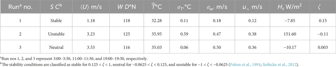
Table 1. Summary of the mean meteorological conditions for the three 30-min runs: friction velocity ($u_{*}$), stability parameter ($\mathrm{\zeta }$), sensible heat flux ($H_t$), stability condition (S C), mean horizontal wind $〈U〉$, wind direction (W D), mean air temperature ($\overline{T}$), temperature fluctuation standard deviations (${\sigma }_{T^{\prime }}$), and vertical velocity fluctuation standard deviations (${\sigma }_{w^{\prime }}$).

2.2 Theoretical considerations

The heat transferred by eddies cross a horizontal surface in the atmosphere, at any height z, is given by Priestley and Swinbank (1947):

$H=\overline{\rho }{C}_p\overline{w\left(T-T_0\right),}(2)$

where $\overline{\rho }$ and $C_p$ are the mean air density (kg m⁻³) and the specific heat capacity of dry air at a constant pressure (J kg⁻¹ K⁻¹), respectively. Here, $w$ is the vertical wind velocity and $T-T_0$ is the temperature change with respect to the environmental temperature (Priestley and Swinbank, 1947) or the base temperature $T_0$ (Webb et al., 1980). Webb et al. (1980) describe the base temperature $T_0$ as “…taken as constant at any given height, representing roughly an assumed initial base temperature from which each element of air is warmed (or cooled) during the vertical transfer of heat supplied (or removed) at the underlying surface.” Henceforth, we use the term “environmental temperature” for $T_0$. If we substitute the mean temperature $\overline{T}$ into Eq. 2, it becomes

$H=\overline{\rho }{C}_p\overline{w}·\left(\overline{T}-T_0\right)+\overline{\rho }{C}_p\overline{w^{\prime }{T}^{\prime }}=∆H+H_t,(3)$

where $T^{\prime }$ represents the temperature fluctuation with respect to the mean temperature $\overline{\mathrm{T}}$. Additionally, we replace $\overline{T}-T_0$ with $∆T$.

In the conventional approach, the first term on the right side of Eq. 3 is usually neglected as small values of $\overline{w}$ exit in the ASL (Webb, 1982) and the difference between the mean and environmental temperature is considered minimal (Webb et al., 1980). However, we demonstrate in the following that this is not the case, as indicated by Mauder et al. (2008, 2020).

First, consider the two terms on the right side of Eq. 3 denoted as $∆H$ and $H_t$. The additional flux $∆H$ is ignored by the conventional EC method that considers only $H_t$, which is determined by the product of the mean vertical velocity and the difference between the mean and environmental temperatures; it does not account for the additional heat transport contributed by anisotropic thermal structures in the ASL. The decomposition of the sensible heat flux in Eq. 3 suggests that the heat flux H is determined by two temperature scales and two velocity scales. It should be noted that both $∆H$ and $H_t$ are generated by atmospheric eddy motion, regardless of the mean flow and velocity fluctuations (Shang et al., 2004).

2.2.1 Environmental temperature ${\mathit{T}}_{\mathbf{0}}$

An air parcel is heated or cooled as it moves between different layers at different heights. For instance, heat is taken away by the parcels ejected upward, and new parcels with lower temperatures sweep in to supply the removed air. Ramps are commonly observed in temperature traces when high-frequency measurements of temperature are taken for the vertical transportation of these thermal structures (Gao et al., 1989; Chu et al., 1996). A sample of temperature traces under various stability conditions is shown in Figure 1 for 23 June 2004 at 11:00. The ramp-like structures occur under both stable and unstable conditions. In this regard, the surface renewal ramp model was first described by Snyder et al. (1996) and further modified by Chen et al. (1997) as a more realistic ramp model. Figure 2 shows the ramp-like model and information to be extracted, as summarized thus:

• The total ramp duration is characterized by the time over which the air temperature changes, Lr (s), and the time over which the air temperature remains unchanged (i.e., quiescent), Lq (s). The thermal structures in the ramp period Lr are responsible for heat, momentum, water vapor, and other gaseous transportation. During the quiescent period Lq between the falling ramp and the formation of the next ramp, the flux exchange is scarce (Chen et al., 1997).

• The amplitude $a_1$ ($a_2$) (°C) of the ramps has the following relations: $a_1>0$ for unstable conditions, $a_2<0$ for stable conditions, and usually $\left|a_1\right|>\left|a_2\right|$.

• Both the warm plumes found in unstable conditions, and the cool plumes that occur under stable conditions in the low ASL are usually driven by instabilities in the velocity layer (Gao et al., 1989; Belmonte and Libchaber, 1996), thus creating the slopes of the ramp-like structures. ${Sl}_1$ and ${Sl}_2$ are the slopes of rising and falling ramps, respectively. Usually, $\left|{Sl}_2\right|>\left|{Sl}_1\right|$.

Figure 1

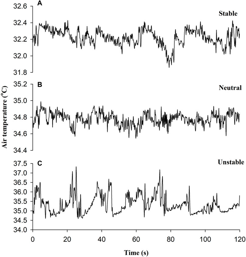
Figure 1. Air temperature (°C) fluctuations observed in a 10-Hz sample for stable (03:00, (A)), neutral (19:00, (B)), and unstable conditions (11:00, (C)) on 23 June 2004.

Figure 2

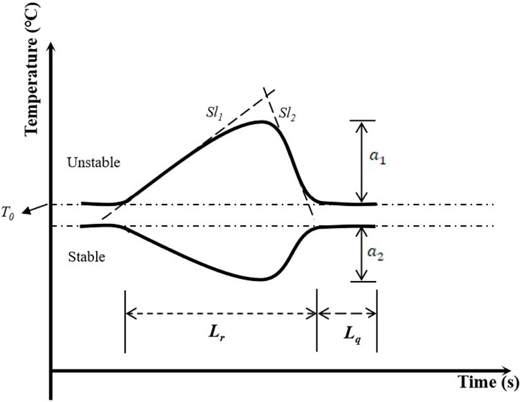
Figure 2. Analysis of the ramp-like model for temperature fluctuations in the atmospheric surface layer (ASL), where $a_1$ ($a_2$) is the amplitude of the air temperature, L_r is the ramp period, L_q is the quiescent time period, T₀ is the environmental temperature, and Sl₁ and Sl₂ are the slopes of the rising and falling ramps, respectively. This figure is re-drawn from Snyder et al. (1996) and Chen et al. (1997).

Here, we take the temperature within the quiescent period Lq as the environmental temperature $T_0$. The reason for this is that the temperature change $T-T_0$ is a very small value during the quiescent period; thus, the air is depleted of heat flux exchange. The probability density function (PDF) of the temperature provides a simple method to evaluate the environmental temperature. A relatively distinct peak in the PDF of temperature fluctuation is likely to be present, even under the condition that a very short period of Lq is included. Thus, we take the most probable temperature within a 30-min period as the environmental temperature $T_0$ (Shang et al., 2004). Here, we do not need to estimate the ramp period Lr or the quiescent period Lq; only the recorded temperature is necessary.

Webb et al. (1980) noted that $T_0$ should be constant at any given height and represents a reference state of temperature from which each element of air is warmed (or cooled) during the vertical transfer of heat supplied (or removed) at the underlying surface. Thus, the thermal structures will supply or remove heat at the given height, but $T_0$ will remain constant. Moreover, the ramps are characterized by the thermal structures, the pass-through of which returns the temperature to a stable level (Figure 2). The statement above serves as the second reason for obtaining $T_0$ by analyzing the measured temperature’s PDF.

The environmental temperature $T_0$ is determined using the following steps:

1) Calculate the temperature fluctuations $T^{\prime }=T-\stackrel{\sim }{T}$, where $\stackrel{\sim }{T}$ is low-pass-filtered by a window function $G\left(t;t_0\right)$, as given by Moncrieff et al. (2004) using Eqs 4 and 5:

$\stackrel{\sim }{T}\left(t\right)={\int }_{{-t}_0}^{t_0}G\left(t^{\prime }-t;t_0\right)T\left(t^{\prime }\right)d{t}^{\prime }(4)$

and

$G\left(t;t_0\right)=\left\{\begin{array}{l}1/2t_0\text{\hspace{1em}for\hspace{0.17em}}\left|t\right|<t_0\\ 0\text{\hspace{1em}for\hspace{0.17em}}\left|t\right|>t_0.\end{array}\right.(5)$

Here, the width of window ($2t_0$) is 30 min and is thus comparable to the common temporal EC method.

2) Evaluate the PDF, denoted as $P\left(T^{\prime }\right),$ of each 30-min temperature fluctuation by clustering the 18,000 measurements within different bins in the same window width of 0.01°C.

3) Identify temperature $T_M^{\prime }$ that corresponds to the maximum of $P\left(T^{\prime }\right)$, where $T_M^{\prime }$ ranges between the minimum and maximum of $T^{\prime }$.

4) Obtain the environmental temperature $T_0$ using Eq. 6:

$T_0\left(t\right)=\stackrel{\sim }{T}\left(t\right)+T_M^{\prime }\left(t\right).(6)$

5) Calculate the difference between the mean and environmental temperature using Eq. 7:

$∆T=\overline{T}-T_0=-T_M^{\prime }\left(t\right).(7)$

3 Results

3.1 $∆\mathit{T}$ for single-point tower measurements

To more accurately illustrate $∆T$ for the measurements, detailed information about the three runs with different stability conditions is described. Table 1 lists the mean meteorological conditions. The stable condition run had a relatively small horizontal wind speed (1.18 ms⁻¹), a small $u_{*}$ (0.12 ms⁻¹), and small ${\sigma }_{T^{\prime }}$ (0.11$℃$) and ${\sigma }_{w^{\prime }}$ (0.18 ms⁻¹). Under unstable conditions, a moderate horizontal wind speed (3.23 ms⁻¹) and a large $u_{*}$ (0.38 ms⁻¹), ${\sigma }_{T^{\prime }}$ (0.59$℃$), and ${\sigma }_{w^{\prime }}$ (0.47 ms⁻¹) were observed. For the neutral condition, the horizontal wind speed was moderate at 3.53 ms⁻¹; large values were recorded for $u_{*}$ (0.36 ms⁻¹) and ${\sigma }_{w^{\prime }}$ (0.50 ms⁻¹), yet ${\sigma }_{T^{\prime }}$ was small (0.06$℃$). All incoming winds of the three runs had nearly the same direction.

Figure 3 shows the PDFs for the temperature fluctuations of the three runs under the different stability conditions. To contrast them more fully, all maximums of the PDFs were normalized to the value of 1. Distinct peaks were found in the PDF distributions for all stability conditions. For the three runs, the differences between the mean and environmental temperatures ($∆T$) were −0.07 °C, 0.29 °C, and 0.01 °C for stable, unstable, and neutral conditions (Table 2), respectively. To understand the dynamic mechanism for $∆T$, detailed information including the skewness of temperature $(S_T=〈{\left(T-\overline{T}\right)}^3〉/{〈{\left(T-\overline{T}\right)}^2〉}^{3/2})$ and vertical velocity $(S_w=〈{\left(w-\overline{w}\right)}^3〉/{〈{\left(w-\overline{w}\right)}^2〉}^{3/2})$ and the skewness of the temperature derivative $(S_T^{\prime }=〈{\left(\partial T/\partial t\right)}^3〉/{〈{\left(\partial T/\partial t\right)}^2〉}^{3/2})$ is also reported in Table 2. Under stable conditions ($\zeta =0.147$), both $S_T$ and $S_w$ were greater than 0. However, under unstable conditions ($\zeta =-0.109$), negative values were found for both $S_T$ and $S_w$. It is known that the skewed distributions of temperature and vertical velocity indicate the nature of the upward thermal structures in the ASL (Chu et al., 1997). Here, the thermal structures under stable and unstable conditions were generated by the instabilities of the velocity layer for $S_T\bullet S_T^{\prime }<0$ (Belmonte and Libchaber, 1996). The vertical movement of thermal structures led to the existence of a non-zero $∆T$. For example, upward warm and cold structures create temperature differences of $∆T>0$ and $∆T<0$, respectively. Good agreement was attained between $∆T$ and the stability conditions such that $∆T<0$ for stable conditions and $∆T>0$ for unstable conditions. Neutral conditions resulted in a $∆T$ value of approximately 0.

Figure 3

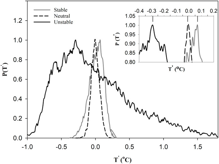
Figure 3. Probability density functions of the temperature fluctuations for the three runs under different stability conditions.

Table 2

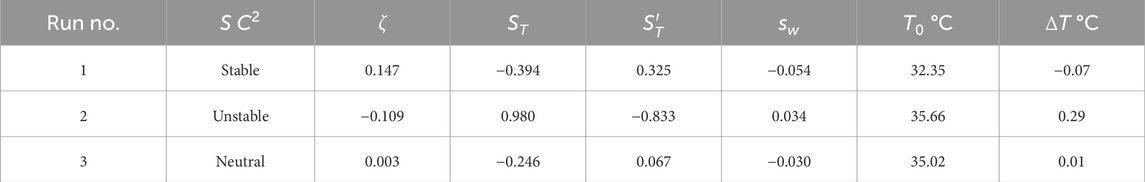
Table 2. Summary of skewness (S) of temperature and vertical velocity, skewness (S’) of the temperature derivative, the environmental temperature ($T_0$), and $∆T$ for the three runs.

Figure 4 shows the variations in $∆T$ for the period 01 June to 10 July 2004. $∆T$ had a maximum value on 04, 12, and 27 June. Generally, positive values of $∆T$ were observed in the daytime hours; at night, $∆T$ was smaller and negative on average (Figure 5). Over the observational period, under the condition of strong solar forcing on sunny days, large $∆T$ ($>$ 0.8°C) was observed on 4 of the 40 days: 04, 12, 14, and 27 June. On 6 June it was rainy, so $∆T$ remained small ($0.19℃$). The diurnal variation of average $∆T$ was consistent with the diurnal variation in the solar radiation: both exhibited strong solar forcing and positive $∆T$ during the day, reached a maximum at noon, but then declined to near 0 or below with negative $∆T$ values at night. The relationships between the stability parameter $\zeta$ and $∆T$ for 40 days are shown in Figures 5B, C. Because the unstable boundary layer was more conducive to the development of thermal structures, large positive values of $∆T$ were usually found under unstable conditions in the daytime. In contrast, the stratification of the boundary layer at night prevented heat and mass exchange between the Earth’s surface and upper air layers, such that small $∆T$ dominated.

Figure 4

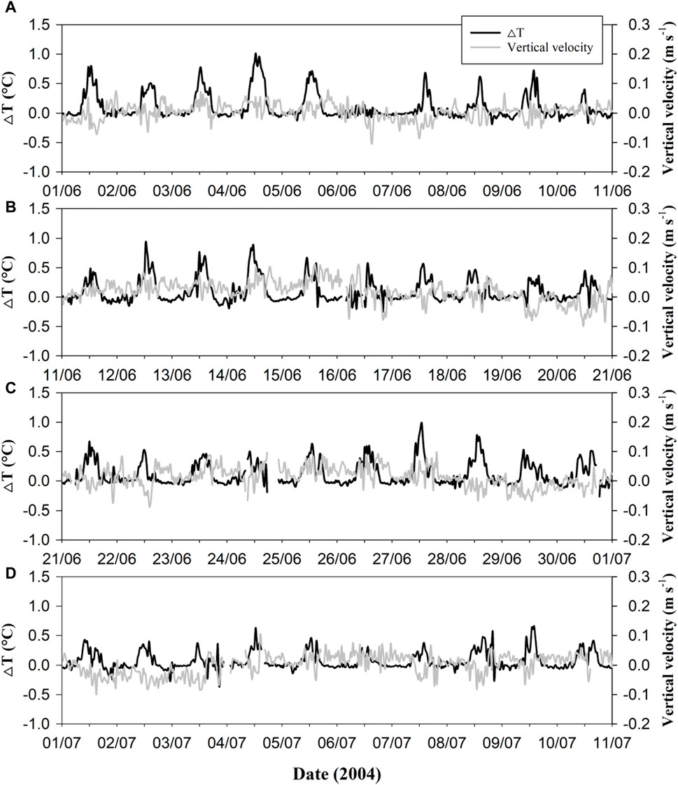
Figure 4. Vertical wind velocities (m s⁻¹) averaged over 30 min and ∆T (°C) for the period (A) 01 June to 10 June 2004, (B) 11 June to 20 June 2004, (C) 21 June to 30 June 2004, and (D) 01 July to 10 July 2004.

Figure 5

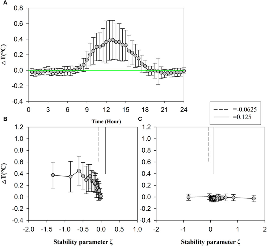
Figure 5. (A) Diurnal variations in the difference between the mean and environmental temperatures ($∆T$), including the standard deviation of the 40 days. (B, C) Plots of $∆T$ vs. the stability parameter ζ for daytime and night, respectively.

3.2 Vertical velocity

Wind data from sonic anemometers are usually transformed into a mean streamline parallel coordinate system to correct for non-zero $\overline{w}$ effects (Wilczak et al., 2001; Finnigan et al., 2003; Dellwik et al., 2010). Following Wilczak et al. (2001), the planar-fit technique was adopted in this study. The corrected vertical velocity can be calculated using Eq. 8:

$w_r=w-b_0-b_1\overline{u}-b_2\overline{v},(8)$

where: $b_0$ is a mean zero offset, possibly due to electronic problems and flow perturbation in the measured vertical velocity; $b_1$ and $b_2$ are wind direction-dependent coefficients; and $\overline{u}$ and $\overline{\mathrm{v}}$ are the longitudinal and lateral velocity, respectively, as measured by a sonic anemometer.

The wind data for 27 to 30 June were selected to determine the linear regression coefficients ($\left.b_0,b_1,\text{and\hspace{0.17em}}{b}_2\right)$ when the sonic anemometer was functioning properly; a wide range of wind directions were found for these four days. The resulting $b_0,b_1,\text{and\hspace{0.17em}}{b}_2$ were 0.0132 m s⁻¹, 0.1197, and 0.0156, respectively.

Figure 4 shows relatively small changes in the vertical velocity ($<$ 0.1 ms⁻¹); notably, the lack of diurnal variation in $\overline{w}$ dominated our measurements. The grasslands had a slight effect on the wind direction, depending on the vertical velocity. However, no distinct vertical component was found even at midday when vertical convection is more likely.

There was a linear relationship between the daily maximum of $∆T$ and the corresponding local vertical velocity (Figure 6). In general, $∆T$ increased with $\overline{w}$. Since $∆T$ was generated by the thermal structures, it can be deemed an indicator of the activity level of those structures in the ASL. The relationship between the maximum $∆T$ and $\overline{w}$ suggests that an increase in the local $\overline{w}$ can result in more active thermal structures. In turn, the development of the thermal structure can be suppressed by terrain gradients, large eddies in the ASL, and/or by local thermal circulations, regardless of whether the local $\overline{w}$ is induced.

Figure 6

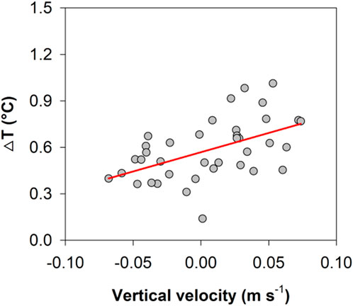
Figure 6. Plot of the maximum of $∆T$ each day versus the corresponding local vertical velocity $\overline{w}$. Red line refers to the linear regression.

3.3 Sensible heat flux

The measurement location was in the tropic monsoon region of southern China. Because measurement commenced in June, the air temperature was relatively high and the diurnal variation in the maximum temperature ranged between 26$℃$ and 38$℃$ (figure not shown). Figure 7 shows the sensible heat flux over the 40-day period. The maximal conventional EC method was used to calculate $H_t$; most values were larger than 80 Wm⁻² at noon, with 04, 14, 17, and 27 June showing a clear sky and strong solar forcing that resulted in flux $H_t$ maxima of 231.4, 232.4, 236.3, and 229.8 Wm⁻², respectively. Relatively frequent rainfall was found within the observation period, and the missing results of $H_t$ were largely induced by rainfall events. Notably, rainfall at noon on 06 June produced a low $H_t$ value of 32.6 Wm⁻².

Figure 7

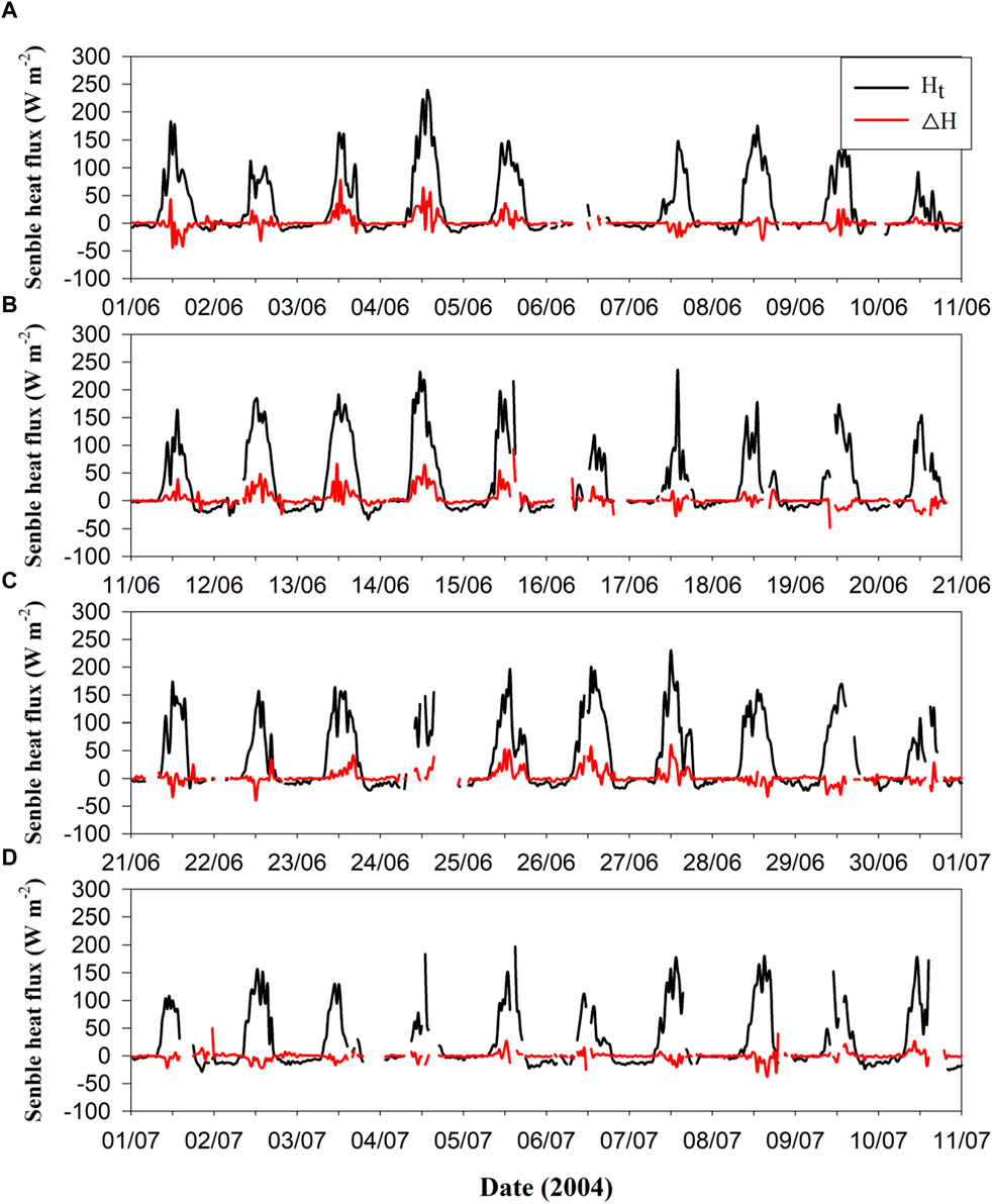
Figure 7. Sensible heat flux estimates for the additional flux ΔH (W m⁻²) and the conventional estimated flux H_t (W m⁻²) for the period 01 June to 10 July 2004. The averaging time is 30 min for the period (A) 01 June to 10 June 2004, (B) 11 June to 20 June 2004, (C) 21 June to 30 June 2004, and (D) 01 July to 10 July 2004.

Large differences (>50 Wm⁻²) between the new method used to estimate the total sensible heat flux $H$ and the conventional EC method used to calculate $H_t$ were found for eight days: 03, 04, 13, 14, 15, 25, 26, and 27 June; $∆H$ for those days were 78.3, 63.4, 66.6, 61.2, 93.5, 51.1, 57.4, and 59.9 Wm⁻², respectively, with the ratio of the ∆H to $H_t$ reaching an astonishing 50.7%, 29.1%, 42.2%, 30.6%, 43.3%, 44.5%, 29.6%, and 26.1%, respectively. Those large differences reached a maximum at noon when strong solar forcing occurred under a large $∆T$ of 0.77, 1.02, 0.39, 0.54, 0.42, 0.48, 0.59, and 0.80 $℃$, respectively. At the same time, a relatively small vertical convection with positive local vertical velocities of 0.07, 0.04, 0.06, 0.08, 0.11, 0.08, 0.07, and 0.07 m s⁻² was observed on these eight days. Notably, on occurrences with large $∆H$, the wind speeds were not large, ranging 1.6 to 3.9 m s^-1, and winds were mostly from the south (Figure 8). In addition to those eight days, additional flux less than 50 Wm⁻² but larger than 30 Wm⁻² was observed for an additional 11 days: 01, 05, 11, 12, 16, 22, 23, and 24 June, and 01, 06, and 08 July.

Figure 8

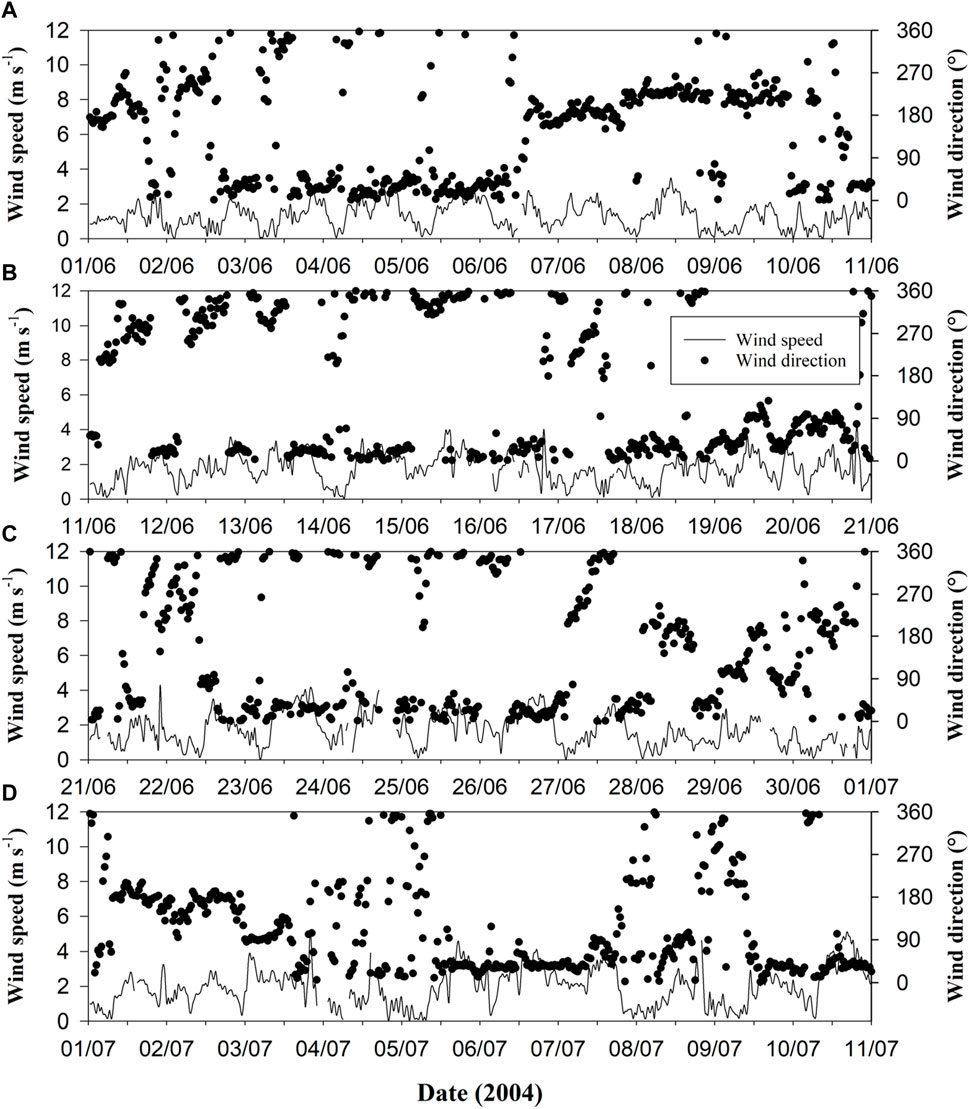
Figure 8. Wind speed (m s⁻¹) and wind direction (°) averaged over 30 min for the period 01 June to 10 July 2004 for the period (A) 01 June to 10 June 2004, (B) 11 June to 20 June 2004, (C) 21 June to 30 June 2004, and (D) 01 July to 10 July 2004.

In addition to the large positive additional flux observed, there were also relatively large negative additional flux values (<−30 Wm⁻²) for some of the other days: −44.0, −32.0, −30.1, −48.2, −33.4, −39.4, −54.9, and −34.3 Wm⁻² for 01, 02, 08, 19, 21, 22, and 28 June, and 08 July, respectively. As with the positive flux, all of the negative flux occurred at noon, with $∆T$ ranging between 0.40 $℃$ and 0.68 $℃$, but with small local subsidence in the vertical velocities ranging between −0.07 and −0.04 m s⁻¹.

Mauder and Foken (2006) indicated an uncertainty of 5% or 10 Wm⁻² from sonic anemometer measurements, using the conventional EC method to estimate the sensible heat flux. The large discrepancies described in sensible heat flux calculated from the conventional EC method and the new EC method at noon in our observations seem plausible as the thermal structures were active at this time of day. The presence of small local vertical velocities resolves these large discrepancies.

4 Discussion

4.1 Reason for the additional flux $∆\mathit{H}$

The conventional EC method was developed under the condition of homogeneous and isotropic turbulence flow, and it was thought able to capture the heat flux contributed by all signals of small-scale motions. The visible contradiction between the prerequisite of the conventional EC method and the widespread anisotropic turbulence in the ASL was the first indication that the conventional EC method may fail to estimate the correct heat flux. The identified thermal structures were responsible for the majority of the vertical heat, momentum, and mass fluxes in the ASL (Gao et al., 1989; Chen et al., 1997). Behind these thermal structures are anisotropic flows. The ability of an anisotropic flow to transport heat differs considerably from that of an isotropic flow.

We obtained the local environmental temperature from the ramp-like structures in our model (Figure 2). If warm (cool) structures occupy the space, then the time mean temperature will be higher (lower) than the environmental temperature. The time scales of the thermal structures are much less than 30 min; thus, they can be captured by the 30-min average operator. Additionally, their spatial scales are not very large, such that the results represent the local heat flux. To measure the additional heat flux contributed by large-scale organized structures, Mauder et al. (2008) used the time–space-averaged temperature as the environmental temperature. However, this may be a limitation of their theory in practice.

When using the most probable temperature within a 30-min period as the environmental temperature, an additional flux due to the transportation of thermal structures could be detected. The additional vertical sensible eddy heat flux $∆H$ is partly decided by the difference between the mean and environmental temperatures, $∆T$. The non-zero $∆T$ presented here was determined by similar existing thermal structures in Figure 2, meaning that both $∆H$ and $H_t$ are a result of the vertical transportation of eddies (Shang et al., 2004). Moreover, even $∆H$ has an inseparable relationship with local vertical convection. A good linear relationship between heat flux $\overline{w^{\prime }{T}^{\prime }}$ and $∆T$ was found (Figure 9B), such that a larger sensible heat flux $H_t$ ($H_t=\rho C_p\overline{w^{\prime }{T}^{\prime }}$) occurred with larger $∆T$, while smaller $∆T$ corresponded to a smaller $H_t$. This linear relationship is also evident when comparing Figures 5A, 9A as both $∆T$ and $H_t$ have the same diurnal variation. The identified thermal structures are responsible for the majority of vertical heat flux in the ASL (Gao et al., 1989; Chen et al., 1997). Large $H_t$ means that the thermal structures are active and an apparent $∆T$ emerges. In these active thermal events, additional fluxes are visible if non-zero $\overline{w}$ occurs. On the other hand, no additional flux exists in the absence of thermal structures, even with strong local vertical convection. Unlike the similar approaches proposed by Lee (1998) and Mauder et al. (2008), in which the former quantifies the convective sensible heat flux by measuring the transported local vertical gradient of the scalar while the latter undertake this by measuring the difference between the time-averaged scalar and the time–space-averaged scalar, $∆H$ and $H_t$ cannot be studied separately. They are both part of the turbulent flux but can be captured by a single-point tower measurement.

Figure 9

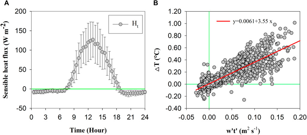
Figure 9. (A) Diurnal variations in the conventional EC method to calculate sensible heat flux ($H_t$), including the standard deviation of 40 days. (B) Plot of $H_t$ vs. $∆T$; the red line refers to the linear regression ($R^2$ = 0.77).

The linear regression relationship from Figure 9 provides a modeled estimation of $∆T$ from the conventional EC method $\overline{w^{\prime }{T}^{\prime }}$ ($H_t$):

$\left[∆T\right]=0.0061+\alpha \left[\overline{w^{\prime }{T}^{\prime }}\right],(9)$

where $\alpha$ is equal to 3.55. The coefficient of determination ($R^2$) of the linear regression is 0.77. Here, $\left[\overline{w^{\prime }{T}^{\prime }}\right]$ is the dimensionless operator, and the coefficient of 3.55 is determined by the thermal structures. The first term on the right side of Eq. 9 will be discarded because zero heat flux exchange means that no thermal structures appeared. We should note that $\alpha$ varies at different underlying surfaces, but the linear relationship in Eq. 9 is reliable.

Substituting Eq. 9 into Eq. 3 leads to the following relationship:

$H_{model}=\left(1+\alpha \left[\overline{w}\right]\right)H_t,(10)$

Based on Eq. 10, it is clear that, once the coefficient is known, the additional flux coinciding with local vertical convection can be resolved. For example, an additional flux of 35.5% of $H_t$ should be included if a slight subsidence of $\overline{w}=0.1\mathrm{m}{\mathrm{s}}^{-1}$ existed for our measurements.

4.2 The role of vertical convection

The additional vertical sensible eddy heat flux $∆H$ is not only decided by the difference between the mean and environmental temperatures $∆T$ but is also sensitive to the local mean vertical wind speed $\overline{w}$. $∆T$ is usually greater than zero in the daytime (Figure 5A); thus, the local subsidence or the local uplift would lead to an underestimation or overestimation of the total sensible heat flux (Figure 10). However, because only small $∆T$ occurs at night, there will be no large underestimation or overestimation. This case somewhat differs from the “cool down” events described by Williams and Hacker (1992) or McNaughton (2004) that underestimate the sensible heat flux for downdrafts as cooler than the ambient air (Mauder et al., 2008). Variations in the vertical velocity perturbation of more than one order larger than $\overline{w}$ lead to a slight subsidence that cannot prevent warm structures from propagating upward due to the instability of the velocity layer as opposed to buoyancy. Closer examination of Figure 5 shows that, although there was slight subsidence at noon on more than 10 of the 40 days, all $∆T$ were positive.

Figure 10

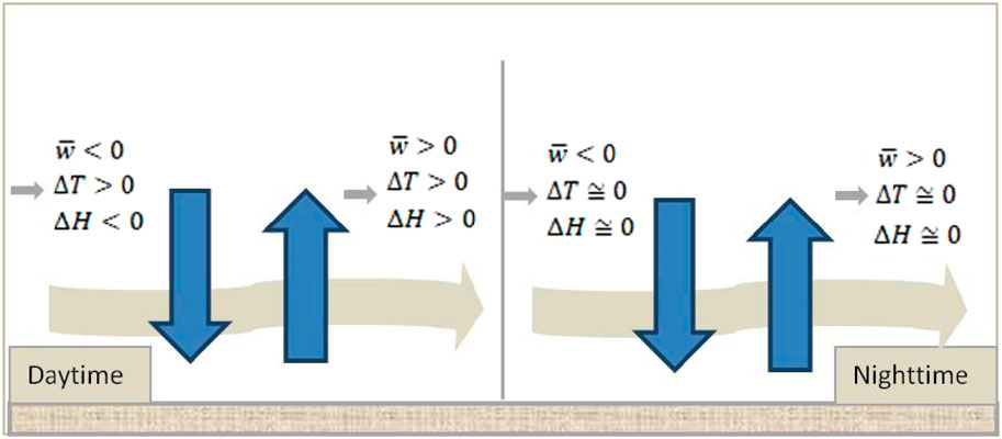
Figure 10. Schematic diagram showing the underestimation or overestimation of total vertical sensible heat flux caused by the thermal structures interacting with local vertical convection in the ASL when using the conventional EC method in Eq. 3.

4.3 The probable role of the method in the energy imbalance problem

It is known that the majority of vertical heat, momentum, and mass fluxes in the ASL are due to the movements of the identified thermal or coherent structures (Qiu et al., 1995; Chen et al., 1997). The creation of these thermal structures is dynamically dominated by the vertical shear of wall-bounded turbulent flows (Gao et al., 1989), and their thermodynamics are dominated by the temperature difference between the upper and bottom boundaries of Earth’s surface or the Rayleigh–Bénard convection (Shang et al., 2004). The structures are usually more pronounced under unstable conditions (Figure 1). Similar ramp patterns of humidity and CO₂ can also be found, and they are both shaped by the turbulence structures in the ASL. Therefore, additional heat flux in the form of latent heat and additional CO₂ transport due to this turbulence should also be considered.

In this study, both the conventional EC estimate and the additional contribution are fluxes transported by the turbulence in the surface layer; that is, the additional contribution is a component of heat transported by the thermal structures but cannot be identified by the conventional EC method. A more intuitive understanding comes from a laboratory experiment of Shang et al. (2004), who compared the heat transports calculated by the EC method and those injected by heater in a turbulent Rayleigh–Bénard convection system. They concluded that the conventional EC estimates can significantly underestimate the injected heat flux under convective conditions, and the underestimated heat transport was captured by the new method (Eq. (3)). The results revealed by Shang et al. (2004) may be inspiration for addressing the energy imbalance problem in the terrestrial surface. The energy imbalance problem was widespread at FLUXNET sites and was most apparent during the day (Wilson et al., 2002). According to Wilson et al. (2002), the difference between the available energy and turbulent energy fluxes reaches its maximum value at noon. Foken et al. (2010) also reported an imbalance of 20%–30% during the daytime in the LITFASS-2003 experiment. Based on the results of our study, the additional contribution $∆H$, which is usually ignored and also usually reaches its maximum value at noon, may be one of the main reasons for the energy imbalance.

The new estimate considers heat transport by thermal structures. These are not unique to the underlying surface of grassland types but are rather a common feature shared by all types of underlying surfaces, indicating the universality of this research. The contribution of thermal structures generated by plant canopies such as grasslands, forests, and crops to heat transport and their related boundary layer energy imbalance problem have received widespread attention (Chen et al., 1997; Castellvi et al., 2008; Holwerda et al., 2021; Cely-Toro et al., 2023). As they are all based on the conventional EC results to study the contribution of thermal structures to heat flux, there is also the inevitable issue of the energy imbalance problem.

Using the conventional EC method, the large-eddy simulation study of the energy imbalance problem by Steinfeld et al. (2007) showed that the imbalances are relatively small (∼5%) at a height of 20 m. However, reports from field experiments indicated a larger imbalance (10%–30%) at lower measurement heights closer to the surface (Wilson et al., 2002; Oncley et al., 2007; Foken et al., 2010). No viable reasons were offered to explain the imbalance difference between the different measured heights.

We describe the presence of thermal structures in the ASL that determine the existing $∆T$. Those structures, without mixing with the surrounding air, create the ramp-like patterns in the model, leading to temperature skewness (Table 2). When the thermal structures propagate into the upper air and mix with the surrounding environment, the thermal structures gradually fade, and a corresponding decrease in $∆T$ occurs. Thus, the value of $∆H$ would also decrease with height while having the same $\overline{w}$ at different heights. This means that, if the ignored $∆H$ is included in the total vertical sensible heat flux, the question of the reduction in the imbalance rate with height may be partly answered. Of course, further study is needed to confirm this premise.

5 Summary

The conventional temporal EC method ($H_t$) usually underestimates the total vertical sensible heat flux, thus contributing to the “energy imbalance problem” in the ASL. A better estimate requires that the environmental temperature is accounted for. Based on the ramp-like model for temperature fluctuations, we used the most probable temperature of each 30-min data run as the environmental temperature. Additional sensible heat flux was detected with our proposed approach in comparison to the conventional EC method. The additional flux ($∆H$), which can be measured by single-point tower measurements, is determined by the difference between the mean and environmental temperatures ($∆T$) and the local mean vertical wind velocity ($\overline{w}$) due to the vertically transported thermal structures in the ASL. Both $∆H$ and $H_t$ are produced by eddies. Measurement data over a grassland surface in southern China from 01 June to 10 July 2004 were used to test the new EC method.

The additional sensible heat flux usually peaked at noon, when solar forcing was strong and the convective boundary was developed. Large underestimations of the sensible heat flux exceeding 50 Wm⁻² were found for 8 of the 40 days of the observational period. For the eight days, large differences between the mean and environmental temperatures (>0.39°C) and small vertical velocities (<0.11 ms⁻¹) were evident. Underestimations which, although smaller, were still significant in the order of 30–50 Wm⁻² were found for 11 other days, as well as a relatively large negative additional flux (<−30 Wm⁻²). A simple model of the interaction between the thermal structures and local vertical convection was developed. The underestimation or overestimation of vertical sensible heat flux was decided by the vertical wind direction in the daytime, while the errors in sensible heat flux were small at night.

The additional flux can be determined once the difference between the mean and environmental temperatures ($∆T$) is resolved. Our results showed that $∆T$, decided by the vertical transportation of anisotropic thermal structures, was predominantly positive during the daytime when the boundary layer was unstable and the thermal structures were active. In the evening, the ASL was neutral or stable and $∆T$ tended to 0, but with slight negative mean values. Thus, $∆T$ can be deemed an activity-level indicator of the thermal structures in the ASL. A good linear relationship with a slope of 3.55 between $∆T$ and $\overline{w^{\prime }{T}^{\prime }}$ was found. Using this linear relationship, a simple model for estimating the total vertical sensible heat flux was proposed. Our measurements indicated an under- or overestimation of 3.55[$\overline{w}/\left(1\bullet \mathrm{m}{\mathrm{s}}^{-1}\right)$] $H_t$ of the total vertical sensible heat flux. The local vertical velocity was vital for resolving the additional flux.

In general, additional sensible heat flux cannot be ignored during the daytime. This may thus be an important reason for the widespread energy imbalance, which is more apparent at noon. In addition, $∆T$ decreases with height as the thermal structures propagate upward. The additional heat flux will decrease at the same time, providing a rational answer to the puzzle of an energy imbalance rate decrease with height. However, additional studies are required for confirmation.

Data availability statement

The raw data supporting the conclusion of this article will be made available by the authors, without undue reservation.

Author contributions

YQ: methodology, visualization, and writing–original draft. XS: conceptualization, funding acquisition, supervision, and writing–review and editing. GC: conceptualization and writing–original draft. ZG: validation and writing–review and editing. XB: investigation and writing–review and editing. LY: formal analysis and writing–review and editing. HM: formal analysis and writing–review and editing.

Funding

The author(s) declare that financial support was received for the research, authorship, and/or publication of this article. The study was mainly supported by the National Key R&D Plan of China under contract nos 2021YFC3101301, 2021YFC2803104, and 2022YFC3104403.

Acknowledgments

The authors are grateful to the Guangzhou Institute of Tropical and Marine Meteorology, CMA, Guangzhou, China, for the available data used in this study.

Conflict of interest

The authors declare that the research was conducted in the absence of any commercial or financial relationships that could be construed as a potential conflict of interest.

Publisher’s note

All claims expressed in this article are solely those of the authors and do not necessarily represent those of their affiliated organizations or those of the publisher, the editors, and the reviewers. Any product that may be evaluated in this article, or claim that may be made by its manufacturer, is not guaranteed or endorsed by the publisher.

References

Belmonte, A., and Libchaber, A. (1996). Thermal signature of plumes in turbulent convection: the skewness of the derivative. Phys. Rev. E 53, 4893–4898. doi:10.1103/physreve.53.4893

PubMed Abstract | CrossRef Full Text | Google Scholar

Bi, X., Gao, Z., Deng, X., Wu, D., Liang, J., Zhang, H., et al. (2007). Seasonal and diurnal variations in moisture, heat, and CO2 fluxes over grassland in the tropical monsoon region of southern China. J. Geophys. Res. 112, D10106. doi:10.1029/2006JD007889

CrossRef Full Text | Google Scholar

Castellvi, F., Snyder, R. L., and Baldocchi, D. D. (2008). Surface energy-balance closure over rangeland grass using the eddy covariance method and surface renewal analysis. Agric. For. Meteorol. 6-7 (148), 1147–1160. doi:10.1016/j.agrformet.2008.02.012

CrossRef Full Text | Google Scholar

Cely-Toro, I. M., Mortarini, L., Dias-Junior, C. D., Giostra, U., Buligo, L., Degrazia, G. A., et al. (2023). Coherent structures detection within a dense Alpine forest. Agric. For. Meteorol. 343, 109767. doi:10.2139/ssrn.4357159

CrossRef Full Text | Google Scholar

Chen, W., Novak, M. D., Black, T. A., and Lee, X. (1997). Coherent eddies and temperature structure functions for three contrasting surfaces. Part I: ramp model with finite microfront time. Boundary-Layer Meteorol. 84, 99–124. doi:10.1023/a:1000338817250

CrossRef Full Text | Google Scholar

Chu, C. R., Parlange, M. B., Katul, G. G., and Albertson, J. D. (1996). Probability density functions of turbulent velocity and temperature in the atmospheric surface layer. Water Resour. Res. 32, 1681–1688. doi:10.1029/96wr00287

CrossRef Full Text | Google Scholar

Dellwik, E., Mann, J., and Larsen, K. S. (2010). Flow tilt angles near forest edges-part 1: sonic anemometry. Biogeosciences 7, 1745–1757. doi:10.5194/bg-7-1745-2010

CrossRef Full Text | Google Scholar

Finnigan, J. J., Clement, R., Malhi, Y., Leuning, R., and Cleugh, H. (2003). A re-evaluation of long-term flux measurement techniques part I: averaging and coordinate rotation. Boundary-Layer Meteorol. 107, 1–48. doi:10.1023/a:1021554900225

CrossRef Full Text | Google Scholar

Foken, T., Mauder, M., Liebethal, C., Wimmer, F. B. F., Leps, J. P., Raasch, S., et al. (2010). Energy balance closure for the LITFASS-2003 experiment. Appl. Climatol. 101, 149–160. doi:10.1007/s00704-009-0216-8

CrossRef Full Text | Google Scholar

Foken, T., Skeib, G., and Ricter, S. H. (1991). Dependence of the integral turbulence characteristics on the stability of stratification and their use of Doppler-Sodar measurements. Z. Meteorol. 41, 311–315.

Google Scholar

Foken, T. M., Gockede, M., Mauder, L. M., Amiro, B., and Munger, W. (2004). “Post-field data quality control,” in Handbook of micrometeorology: a guide for surface flux measurement and analysis. Editors X. Lee, W. J. Massman, and B. Law (Dordrecht: Kluwer Academic Publishers), 182–208.

Google Scholar

Gao, W., Shaw, R. H., and Paw U, K. T. (1989). Observation of organized structure in turbulent flow within and above a forest canopy. Boundary-Layer Meteorol. 47, 349–377. doi:10.1007/bf00122339

CrossRef Full Text | Google Scholar

Garcia-Santos, V., Cuxart, J., Jimenez, M. A., Martinez-Villagrasa, D., Simo, G., Picos, R., et al. (2019). Study of temperature heterogeneities at sub-kilometric scales and influence on surface-atmosphere energy interactions. IEEE Trans. Geosci. Remote Sens. 57, 640–654. doi:10.1109/tgrs.2018.2859182

CrossRef Full Text | Google Scholar

Holwerda, F., Guerrero-Medina, O., and Meesters, A. G. C. A. (2021). Evaluating surface renewal models for estimating sensible heat flux above and within a coffee agroforestry system. Agric. For. Meteorol. 308-309, 108598. doi:10.1016/j.agrformet.2021.108598

CrossRef Full Text | Google Scholar

Kaimal, J. C. C., and Finnigan, J. J. (1994). Atmospheric boundary layer flows: their structure and measurement. New York: Oxford University Press.

Google Scholar

Lee, X. (1998). On micrometeorological observations of surface-air exchange over tall vegetation. Agric. For. Meteorol. 91, 39–49. doi:10.1016/s0168-1923(98)00071-9

CrossRef Full Text | Google Scholar

Leuning, R., van Gorsel, E., Massman, W. J., and Isaac, P. R. (2012). Reflections on the surface energy imbalance problem. Agric. For. Meteorol. 156, 65–74. doi:10.1016/j.agrformet.2011.12.002

CrossRef Full Text | Google Scholar

Mauder, M., Cuntz, M., Drüe, C., Graf, A., Rebmann, C., Schmid, H. P., et al. (2013). A strategy for quality and uncertainty assessment of long-term eddy-covariance measurements. Agric Meteorol 169, 122–135. doi:10.1016/j.agrformet.2012.09.006

CrossRef Full Text | Google Scholar

Mauder, M., Desjardins, R. L., Pattey, E., Gao, Z., and van Haarlem, R. (2008). Measurement of the sensible eddy heat flux based on spatial averaging of continuous ground-based observations. Boundary-Layer Meteorol. 128, 151–172. doi:10.1007/s10546-008-9279-9

CrossRef Full Text | Google Scholar

Mauder, M., Desjardins, R. L., Pattey, E., and Worth, D. (2010). An attempt to close the daytime surface energy balance using spatially-averaged flux measurements. Boundary-Layer Meteorol. 136, 175–191. doi:10.1007/s10546-010-9497-9

CrossRef Full Text | Google Scholar

Mauder, M., and Foken, T. (2006). Impact of post-field data processing on eddy covariance flux estimates and energy balance closure. Meteorol. Z. 15, 597–609. doi:10.1127/0941-2948/2006/0167

CrossRef Full Text | Google Scholar

Mauder, M., Foken, T., and Cuxart, J. (2020). Surface-energy-balance closure over land: a review. Boundary-Layer Meteorol. 177, 395–426. doi:10.1007/s10546-020-00529-6

CrossRef Full Text | Google Scholar

Mauder, M., and Zeeman, M. J. (2018). Field intercomparison of prevailing sonic anemometers. Atmos. Meas. Tech. 11, 249–263. doi:10.5194/amt-11-249-2018

CrossRef Full Text | Google Scholar

McNaughton, K. G. (2004). Turbulence structure of the unstable atmospheric surface layer and transition to the outer layer. Boundary-Layer Meteorol. 112, 199–221. doi:10.1023/b:boun.0000027906.28627.49

CrossRef Full Text | Google Scholar

Oncley, S. P., Foken, T., Vogt, R., Kohsiek, W., DeBruin, H. A. R., Bernhofer, C., et al. (2007). The energy balance experiment EBEX-2000. Part I: overview and energy balance. Boundary-Layer Meteorol. 123, 1–28. doi:10.1007/s10546-007-9161-1

CrossRef Full Text | Google Scholar

Priestley, C. H. B., and Swinbank, W. C. (1947). Vertical transport of heat by turbulence in the atmosphere. Proc. R. Soc. A 189, 543–561.

Google Scholar

Qi, Y., Shang, X., Chen, G., Gao, Z., and Bi, X. (2015). Using the cross-correlation function to evaluate the quality of eddy-covariance data. Boundary-Layer Meteorol. 157, 173–189. doi:10.1007/s10546-015-0060-6

CrossRef Full Text | Google Scholar

Richardson, A. D., Aubinet, M., Barr, A. G., Hollinger, D. Y., Ibrom, A., Lasslop, G., et al. (2012). “Uncertainty quantification,” in Eddy covariance: a practical guide to measurement and data analysis. Editors M. Aubinet, T. Vesala, and D. Papale (Dordrecht: Springer), 173–210.

CrossRef Full Text | Google Scholar

Shang, X.-D., Qiu, X.-L., Tong, P., and Xia, K.-Q. (2003). Measured local heat transport in turbulent Rayleigh-Bénard convection. Phys. Rev. Lett. 90, 074501. doi:10.1103/physrevlett.90.074501

PubMed Abstract | CrossRef Full Text | Google Scholar

Shang, X.-D., Qiu, X.-L., Tong, P., and Xia, K.-Q. (2004). Measurements of the local convective heat flux in turbulent Rayleigh-Bénard convection. Phys. Rev. E 70, 026308. doi:10.1103/physreve.70.026308

PubMed Abstract | CrossRef Full Text | Google Scholar

Siebicke, L., Hunner, M., and Foken, T. (2012). Aspects of CO2 advection measurements. Theor. Appl. Climatol. 109, 109–131. doi:10.1007/s00704-011-0552-3

CrossRef Full Text | Google Scholar

Snyder, R. L., Spano, D., and Paw U, K. T. (1996). Surface renewal analysis for sensible and latent heat flux density. Bound. Layer. Meteorol. 77, 249–266. doi:10.1007/bf00123527

CrossRef Full Text | Google Scholar

Steinfeld, G., Letzel, M. O., Raasch, S., Kanda, M., and Inagaki, A. (2007). Spatial representativeness of single tower measurements and the imbalance problem with eddy-covariance fluxes: results of a large-eddy simulation study. Boundary-Layer Meteorol. 123, 77–98. doi:10.1007/s10546-006-9133-x

CrossRef Full Text | Google Scholar

Webb, E. K. (1982). On the correction of flux measurements for effects of heat and water vapour transfer. Boundary-Layer Meteorol. 23, 251–254. doi:10.1007/bf00123301

CrossRef Full Text | Google Scholar

Webb, E. K., Pearman, G. I., and Leuning, R. (1980). Correction of the flux measurements for density effects due to heat and water vapour transfer. Quart. J. R. Met. Soc. 106, 85–100.

CrossRef Full Text | Google Scholar

Wilczak, J. M., Oncley, S. P., and Stage, S. A. (2001). Sonic anemometer tilt correction algorithms. Boundary-Layer Meteorol. 99, 127–150. doi:10.1023/a:1018966204465

CrossRef Full Text | Google Scholar

Williams, A. G., and Hacker, J. M. (1992). The composite shape and structure of coherent eddies in the convective boundary-layer. Boundary-Layer Meteorol. 61, 213–245. doi:10.1007/bf02042933

CrossRef Full Text | Google Scholar

Wilson, K., Goldstein, A., Falge, E., Aubinet, M., Baldocchi, D., Berbigier, P., et al. (2002). Energy balance closure at FLUXNET sites. Agric. For. Meteorol. 113, 223–243. doi:10.1016/s0168-1923(02)00109-0

CrossRef Full Text | Google Scholar