Methane pumping by rapidly refreezing lead ice in the ice-covered Arctic Ocean

1 Introduction

Climate warming impacts Arctic regions 2–4 times faster than the global average (Rantanen et al., 2022). Drastic sea ice losses during summer result in an annual reduction of the September minimum sea ice extent of approximately 25% below the 1981–2010 average and a thinning rate of approximately 10% per decade (Kwok, 2018; Stroeve and Notz, 2018). Most of the thinning is caused by a shift from thicker multiyear ice to thinner first-year ice. Accelerating sea ice drift contributes further to the thinning with shorter residence times of the ice in the central Arctic (Kwok, 2018; Krumpen et al., 2019; Sumata et al., 2023). Sea ice dynamics, that is, the ridging and rafting of colliding floes and ice floes moving apart, create a heterogeneous ice cover with ridges and leads. Leads often cyclically open and close over intervals ranging from days to months (Willmes et al., 2023). Leads are particularly important sites of new ice formation in winter because sea ice growth is faster in open water than below the thicker ice of older floes due to the reduced insulation of ice. Therefore, quick new ice formation in leads contributes up to 30% to the Arctic sea ice mass balance (Kwok et al., 2006; von Albedyll et al., 2022), although leads cover an area of less than 5% of the Arctic sea ice during the freeze period (Wadhams, 2000; Reiser et al., 2020). Recently, the high relevance of leads for the polar climate resulted in increased attention on lead areal fractions in sea ice modeling studies (e.g., Wilchinsky et al., 2015; Zhang et al., 2021; Ólason et al., 2021; Boutin et al., 2023).

In addition to the relevance for the sea ice mass balance, these dynamic processes are associated with a cascade of feedback altering the entire Arctic environmental system, including potential changes in gas and matter fluxes at the air–ocean interfaces (Serreze and Barry, 2011). To date, global coupled models mainly treat the transfer of climate-relevant gases based on fluxes derived from open water measurements and restricted by the area annually or seasonally covered by ice (Torsvik, 2023). Observational studies on methane pathways within sea ice and the exchange at the ocean–ice and air–ice interfaces are scarce and mostly spatially restricted to the marginal ice zone or fast ice areas reported to be affected by local methane sources (Kiditis et al., 2010; Zhou et al., 2013; Zhou et al., 2014; Verdugo et al., 2021; Silyakova et al., 2022; Vinogradova et al., 2022). However, enhanced fluxes of climate-relevant gases from open sea ice leads and cracks in the atmosphere are also described from the central Arctic (Kort et al., 2012; Steiner et al., 2013). More recently, a winter study on refrozen leads revealed physical properties in newly formed lead ice, temporarily favoring an ice-to-air methane flux (Silyakova et al., 2022). While newly formed ice inhibits direct fluxes from the ocean to the atmosphere through leads within hours after opening, refrozen leads exist for days to weeks. Therefore, we suggest that newly formed ice may act as an important pathway for methane transfer in winter. Gas transport within sea ice strongly depends on brine mobility, which decreases with decreasing temperature (Cox and Weeks, 1983; Weeks and Ackley, 1986; Golden et al., 2007; Tison et al., 2017; Crabeck et al., 2019).

In order to evaluate the potential impact of freeze conditions on methane pathways in lead ice and its interfaces, we carried out in situ observations of ice growth during the 2019–2020 Multidisciplinary Drifting Observatory for the Study of Arctic Climate (MOSAiC) drift expedition in the central Arctic (Figure 1). The MOSAiC was a yearlong drift expedition with the purpose of studying the changing Arctic climate system to improve process understanding and model representations of this system (Nicolaus et al., 2022; Rabe et al., 2022; Shupe and Rex, 2022). In a previous study, we described the temporal changes and spatial variability of physical ice properties of different ice types during sea ice growth (Angelopoulos et al., 2022). In the present process study, we investigate changes in physical and chemical properties in newly formed lead ice from the moment of a lead opening through the period of refreezing and ice growth until the closing of the lead by rafting and ridging. Measurements of the same ice were carried out on a weekly basis over a 2-month period from January to March 2020 (Figure 1). These measurements included lead ice temperature and salinity profiles, calculations of the methane solubility capacity (MSC) and methane saturation between lead ice, seawater, and the atmosphere, and the analysis of methane concentration and δ¹³C–CH₄ values in lead ice and surface seawater. We observed stepwise freeze-induced shifts of the physical properties in lead ice that influenced the methane uptake and release at its interfaces, ultimately affecting methane pathways in winter in the high Arctic.

Figure 1

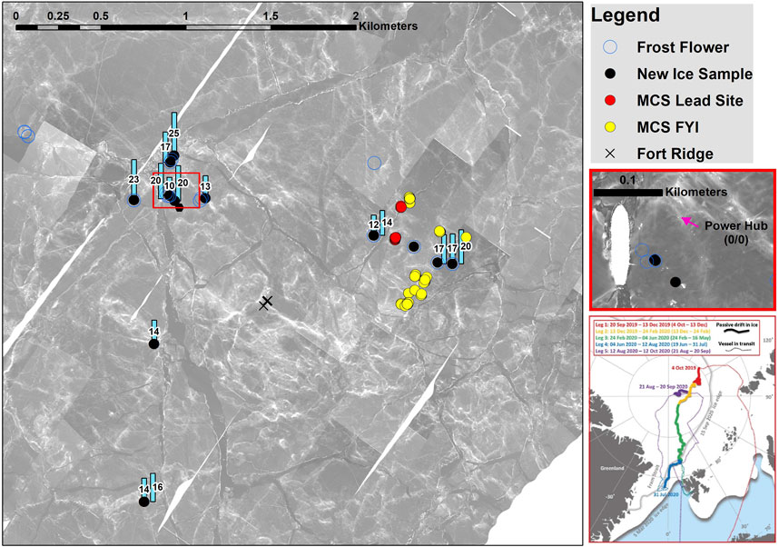
Figure 1. Right side, thin red frame: Track of RV Polarstern during the 2019–2020 MOSAiC drift expedition. Colored line segments show the drift trajectory of different cruise legs on the background of the sea ice extent in March 2020 (Nicolaus et al., 2022). Lead ice sampling occurred on Leg 2 and Leg 3 (yellow and green line) north of 85°N. Large panel: Locations of lead ice sampling on the main coring site (MCS) in the Central Observatory (area around the ship). The ship’s position is within the red square on the right side. Red dots comprise measurements on the same lead ice site on seven dates between 6 January and 7 March 2020, a 2-month observation period. Sampling started 2 days after lead opening and ended as the sampling site disappeared by ridge formation on 8 March 2020. MCS FYI: sampling position of first-year ice at the main coring site. Black dots and blue circles show spots of thin new ice and frost flowers sampled 2–3 days after formation. The blue rectangles give the surface salinity on new ice spots.

2 Methods

2.1 Seawater and lead ice sampling

Seawater samples were taken at a 2 m depth underneath the MOSAiC ice floe using a CTD rosette in the main oceanography tent (Rabe et al., 2022). Bubble-free seawater was collected in 500-mL glass vials that were sealed with rubber stoppers and crimped with aluminum caps. Lead ice coring followed the ice coring procedures of MOSAiC (Angelopoulos et al., 2022). In short, at least three lead ice cores 20–50 cm apart were taken using a Kovacs Mark II 9 cm ice core drill. At each sampling site and day, the first ice core was used for in situ temperature measurements. Thereafter, two cores for the analyses of methane concentration, the stable carbon isotopic signature of methane (δ¹³C–CH₄) and salinity, were taken. Once transferred onboard, the cores were immediately cut into 10-cm slices. Each slice was melted in a gas-tight Tedlar bag after evacuating the air therein in darkness at 4°C. Pieces of thin new ice and frost flowers were cut using a knife and collected with a spittle, respectively, and directly saved in Tedlar bags. Once melted, the meltwater was collected in 500-mL glass vials sealed with rubber stoppers and crimped with aluminum caps. In the following, seawater and melted lead ice samples were processed using the same procedure. In the sample bottles, a headspace was created by injecting 20 mL of hydrocarbon-free synthetic air while, at the same time, water was pushed out via a second needle to balance the pressure. After the gas and water were allowed to come to equilibrium by shaking, the headspace was subsampled with a gas-tight syringe (SGE, Victoria, Australia), and the sample was immediately injected into the small sample isotope module (SSIM, see Section 2.2).

2.2 Analyses of methane concentration and δ¹³C–CH₄ ratios

Methane concentrations and stable carbon isotope ratios (δ¹³C–CH₄) of seawater and bulk ice samples were determined using a Picarro G2132-i cavity ring-down spectrometer coupled to a small sample isotope module (SSIM) (Picarro, Santa Clara, California, USA). The SSIM is a sample inlet system used to analyze discrete samples. The SSIM coordinator software was run in high-precision mode, with a syringe injection setting, and on dilution with hydrocarbon-free air to account for our analysis procedures. The Picarro G2132-i runs with a flow rate of approximately 25 mL/min. For calibration, we used standard gas mixtures with concentrations of 2 ppm, 5 ppm, and 10 ppm (Linde Company) and standard gas mixtures with isotopic ratios of −25‰, −45‰, and −69‰ vs. VPDB (Airgas Company). Considering the complete sampling procedure, the overall total uncertainty was ±5% estimated in duplicate. In addition to this uncertainty, we cannot exclude a concentration-dependent effect on our isotopic ratio measurements (Rella et al., 2015; Uhlig and Loose, 2017; Pohlmann et al., 2021) because many of our measurements were made on samples with mixing ratios <1.2 ppm CH₄ (Supplementary Figure S1). Future studies using a Picarro gas analyzer should use isotopic gas standards spanning the full range of mixing ratios observed in samples in order to isolate the concentration-dependent effect and improve the absolute accuracy of the isotopic ratio measurements.

2.3 Analyses of water and ice temperature and salinity

Surface seawater temperature and salinity at depths of 2 m were continuously measured along the drift track by two thermosalinographs (SBE21, Sea-Bird GmbH) installed in the hull of RV Polarstern (Haas et al., 2021). The temperature and bulk salinity of the lead ice cores were measured according to procedures described in Angelopoulos et al., 2022. In short, ice temperatures were measured in 4.5 cm deep, narrow holes drilled into the core at intervals of 5 cm from the bottom to the top of the ice immediately after the cores were retrieved. Bulk salinity was analyzed on melted subsamples using a WTW 193 Cond 3151 salinometer equipped with a TetraCon 325 four-electrode conductivity cell.

3 Results

3.1 Calculations

3.1.1 Brine volume fraction

The calculation of the brine volume fraction from the ice temperature and salinity data follows Cox and Weeks (1983) according to Eq. 1. To calculate the sea ice density (ρ), the pure ice density as a function of temperature (T) was first estimated from Fukusako (1990). The equation for sea ice density considers temperature-dependent phase equilibrium relationships from Assur (1960) for brine salinity (B_s) and the ratio (k) of the mass of solid salts to the mass of dissolved salts in the brine. We assumed no air volume when implementing the sea ice density. The BVF was calculated from Eq. 1, where ρ is sea ice density, S_i is sea ice salinity, F₁(T) = ρ_b B_s(1+k), and ρ_b is brine density. Brine salinity, density, and the amount of solid salts all vary as a function of temperature (see also Angelopoulos et al., 2022).

$BVF=\frac{\rho S_i}{F_1\left(T\right)}(1)$

The BVF decreases as the temperature and bulk salinity of ice decrease. Here, we adopt the hypothesis of the law of fives, which states that when BVF is above 5%, the ice is permeable, and brine moves in channels, but when BVF falls below 5%, the ice becomes impermeable for brine movement, and brine inclusions disconnect (Golden et al., 2007).

3.1.2 Rayleigh number

The Rayleigh (Ra) number is a dimensionless value that characterizes a fluid’s flow regime and describes the susceptibility of sea ice to brine convection (e.g., Notz and Worster, 2009; Zhou et al., 2013). In the literature, the critical Ra number for which the sea becomes unstable to convection varies between 2 and 10. However, lower values are typically used for field studies (Gourdal et al., 2019). We calculate a local Ra number for different sampling points in the ice column to help determine how and when brine gravity drainage influenced the lead ice salinity profiles. The driving variables affecting the local Ra number are the ice depth, the brine salinity gradient between the ice depth and seawater, and the effective sea ice permeability. We followed the same approach from Angelopoulos et al. (2022) to ensure consistency between the characterizations of first-year ice (FYI), second-year ice, and new lead ice at the different MOSAiC sites. Like Angelopoulos et al. (2022), the physical constants needed for the Ra calculation were adopted from Gourdal et al. (2019).

3.1.3 Methane solubility capacity in seawater and lead ice

In this work, we have defined the methane solubility capacity (MSC in molL⁻¹) as the thermodynamic capacity to dissolve methane in a liquid. Following the dependency of Henry’s solubility coefficient (K_H in mol L⁻¹ atm⁻¹) on temperature T) and salinity S), the equilibrium MSC in seawater is given by

${\text{MSC}}_{\text{SW}}=\mathrm{P}*{\mathrm{K}}_{\mathrm{H}\left(\mathrm{T},\mathrm{S}\right)},(2)$

where P is the partial pressure of methane in the overlying atmosphere (in atm). The T and S dependency of K_H can be derived from the measured Bunsen solubility coefficient (β), which describes the volume of pure dry gas reduced to standard temperature and pressure (STP; 0°C and 1 atm) that will dissolve in a volume of water at ambient T exposed to a gas partial pressure of 1 atm. The Bunsen coefficients for methane have been measured for various temperatures and salinities (Wiesenburg and Guinasso, 1979) and can be easily converted into Henry’s solubility by K_H = β/V_M, where V_M is the molar volume of the gas at STP (L/mol). Assuming that the total atmospheric pressure is equal to 1 atm and the relative humidity is 100%, Eq. 2 can be written in the form most often used for solubility calculations of methane in moist air:

$\text{MSC}=\frac{\mathrm{\beta }}{{\mathrm{V}}_{\mathrm{M}}}*\left(1-{\mathrm{P}}_{\text{vp}}\right)*{\mathrm{f}}_{\mathrm{G}},(\mathrm{2a})$

where P_vp is the saturation vapor pressure of the water (atm) and f_G is the dry mole fraction of the gas in the atmosphere. Based on measured Bunsen solubility coefficients reported in the literature, Wiesenburg and Guinasso (1979) have shown that MSC can be described as a function of temperature, salinity, and mole fraction of methane in a dry atmosphere by using a single equation. For the calculation of MSC in nmol L⁻¹, we use Equation 7 along with the coefficients in the second row of Table VI in Wiesenburg and Guinasso (1979) to obtain the equation for the atmospheric equilibrium solubility:

$\begin{array}{ll}\hfill \ln \text{MSC}& =\ln {\mathrm{f}}_{\mathrm{G}}-415.2807+596.8104*\left(\frac{100}{\mathrm{T}}\right)\hfill \\ \hfill & +379.2599*\ln \left(\frac{\mathrm{T}}{100}\right)-62.0757*\left(\frac{\mathrm{T}}{100}\right)\hfill \\ \hfill & +\mathrm{S}*\left[-0.05916+0.032174*\left(\frac{\mathrm{T}}{100}\right)-0.0048198*{\left(\frac{\mathrm{T}}{100}\right)}^2\right],\hfill \end{array}(\mathrm{2b})$

where T is the absolute temperature in Kelvin and S is the salinity in parts per thousand. MSC increases with decreasing temperature and salinity. However, the temperature effect clearly outweighs the salinity effect when cooling to the freezing point occurs in polar surface water. Note that K_H (or β) is defined within the range of −2 < T < 40°C and 0 < S < 40 (Wiesenburg and Guinasso, 1979), but it has been postulated to remain valid for the potentially much lower temperatures of brine found in sea ice (Zhou et al., 2013; Crabeck et al., 2019).

When seawater begins to freeze, the methane dissolved in seawater becomes incorporated in liquid brine at the ice–seawater interface, and the brine temperature is equal to the temperature of the surrounding ice. Within the liquid brine, dissolved methane migrates within the brine channels as long as the ice is still permeable. With decreasing ice and brine temperatures, BVF decreases, and the ice becomes impermeable when BVF <5% (Golden et al., 2007). Brine is then trapped in discrete pockets. Therein, liquid brine remains in thermodynamic equilibrium with the ice matrix, whose temperature controls the brine volume and salinity. During ongoing cooling, brine pockets shrink as water freezes onto the walls of the pockets, thereby increasing the internal brine salinity (iB_S). The increase in iB_S due to the decrease in temperature is described by

${\text{iB}}_{\mathrm{s}}=1.2-21.8*\mathrm{T}-0.919*{\mathrm{T}}^2-0.0178*{\mathrm{T}}^3.(3)$

As exclusively defined by ambient ice temperature, iB_s increases with decreasing temperature (Notz, 2005). Replacing S by iB_s, Eq. 2b predicts a reduced MSC in enclosed brine pockets compared to the MSC in seawater (MSC-I; Figure 2A).

Figure 2

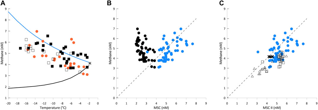
Figure 2. (A): Calculated methane solubility capacity (MSC) and measured methane concentrations in lead ice versus brine temperature. The black star shows the MSC of seawater calculated for the freezing point. Curved lines show MSCs calculated using the two methods. MSC-I (black line) with brine salinity in equilibrium with ambient temperature (iB_s; Eq. 3; related to closed brine pockets in impermeable ice) and MSC-II (blue line) with brine salinity equal to seawater salinity (32 PSU, Eq. 2; related to open brine channels in permeable ice). Orange dots and black squares represent measured concentrations of all ice samples from the first and second month of the time series, respectively. Open squares are related to 2–3-day-old lead ice spots (for locations, see Figure 1). (B) Measured methane concentrations vs. calculated MSCs (MSC-I in black; MSC-II in blue dots). The dotted line represents 100% saturation. Areas to the left and right of this line represent super- and undersaturation, respectively. Calculations with MSC-I result in clear supersaturation, while with MSC-II, they result in scattering around the saturation line. (C) Methane concentration in seawater (crosses), thin new ice (open squares), lead ice from the time series (blue dots), and triangles (frost flowers) vs. MSC-II. The gray line represents 100% saturation. A strong freeze induced enhanced MSC-II levels in thin new ice relative to seawater. The increase in concentration reflects an uptake of gaseous/re-dissolved methane initiated by the increase in MSC-II during a freeze.

The situation is different, however, in bottom ice, at the ice–seawater interface, and also in new lead ice that is still permeable. During the transition period from seawater conditions to conditions present in impermeable ice, dissolved methane still migrates with the brine in open brine channels as long as the BVF is above 5%. In an open brine channel system, brine salinity might still be close to seawater salinity. Furthermore, a fast and strong decrease in temperature could place the brine out of the equilibrium state with the ice matrix because diffusion of temperature is faster than diffusion of salt; that is, brine salinity adjusts more slowly to colder ambient conditions than brine temperature. Therefore, the brine could become temporarily supercooled below its equilibrium freezing point. This mechanism would decrease the temperature in the liquid brine faster than it increases the brine’s salinity. Then, the MSC in brine is still mainly controlled by temperature comparable to MSC in seawater. Because there is no liquid-to-ice phase transition in the formation of supercooled water, we assume that the calculation of MSC following Wiesenburg and Guinasso (1979) remains valid. This is similar to cloud water droplets, which can persist in a supercooled state to below −37°C (Rosenfeld and Woodley, 2000), and to sodium chloride at the interface of snow, which can exist as supercooled liquid down to −32°C (Bartels-Rausch et al., 2021). However, it is not known if a supercooled phase occurs at the interface of brine with the ice matrix. Here, we assume the possibility of a transient (metastable) supercooled state of the liquid brine, which will eventually destabilize to form ice and thereby trap methane in the ice matrix or liquid brine. In particular, we suggest that this process is important in the beginning of sea ice formation in leads before the time of complete brine entrapment, where brine is basically seawater of salinity 32 PSU in contact with the very cold atmosphere. Supercooling was also observed in seawater underneath Arctic winter sea ice (Katlein et al., 2020). The observed water temperatures of only 0.01–0.02 K below the respective seawater freezing point (Katlein et al., 2020) probably represent a final residual supercooled state at the end of ice floe formation.

Using seawater salinity instead of brine salinity for the calculation of MSC (MSC-II) results in a net increase in MSC in permeable lead ice compared to seawater, which is in good agreement with our measured concentrations (Figure 2A). By comparison, calculations carried out for MSC-I and MSC-II show the range between the lowest and highest solubility capacity that can be expected in newly forming lead ice (Figure 2A). We suggest experimental analyses to validate the relationship between changing freeze conditions and the MSC under special consideration of sea ice permeability.

3.1.4 Methane saturation in seawater and lead ice

The ratio between measured and calculated concentrations at the atmospheric equilibrium gives the methane saturation (Figure 2B). As atmospheric equilibrium concentration, we used an atmospheric mole fraction f_G = 1.95 × 10⁻⁶ (NOAA global sampling networks http://www.esrl.noaa.gov). Differences in saturation reflect the contrasting effect of assuming equilibrium with brine salinity (MSC-I; Eq. 3) or seawater salinity (MSC-II; Eq. 2). The balancing net effect of decreasing temperature and increasing iB_s on MSC results in MSC-I being smaller than MSC_SW, ultimately causing supersaturation in brine.

By comparison, MSC-II reflects the dominance of the temperature effect on MSC in newly formed and still-permeable lead ice. Using MSC-II promotes scattering along the saturation line, which mirrors the effect of temperature decrease and reveals the trend of increasing concentration during ongoing cooling. In the following, we are using the MSC-II calculations because they better agree with our measurements. That is, MSC-II better describes the effect of relative changes in MSC induced by fast, strong cooling in still-permeable lead ice (see Discussion) (Figure 2B).

3.2 Phases of lead ice formation—the time series

We analyzed the concentration and stable carbon isotope ratio of methane in lead ice and used the methane concentration and δ¹³C–CH₄ ratio in surface seawater immediately measured before lead opening as our values at time zero (t = 0). Surface seawater was in equilibrium or slightly supersaturated (less than 10%) relative to the atmosphere, while the δ¹³C–CH₄ ratios of dissolved methane in seawater deviated by 8‰–10‰ ¹³C-enrichment from the Arctic atmospheric equilibrium δ¹³C–CH₄ signature (≈−47.5‰; White et al., 2018).

Figure 3 shows lead ice measurements during the 2-month sampling period. We divided this period into five different phases to highlight different predominant processes of lead ice evolution in the following subsections.

Figure 3

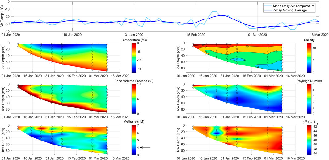
Figure 3. Time series of air temperature above and physical and chemical properties within growing lead ice at our main sampling site between 6 January and 7 March 2020 (location: see Figure 1). The black arrow in the bottom left panel marks the methane concentration in seawater.

3.2.1 Phase I: initial lead ice formation

The first sampling occurred 2 days after the lead opened on 4 January. During this 2-day period, the ice grew 15 cm thick, and its surface temperature decreased from seawater temperature to −5.9°C. The complete ice layer was still permeable with BVFs >10% (Figures 3, 4). The temperature decrease increased the MSC-II therein by approximately 20% compared to the MSC in seawater (Figure 2A). However, our measurements show that methane was not undersaturated during this time. In addition, we observed δ¹³C–CH₄ values depleted in ¹³C in lead ice compared to the marine methane background (Figure 3).

Figure 4

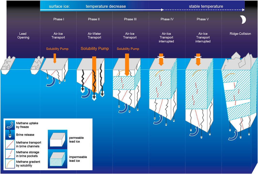
Figure 4. Temporal development of growing lead ice between lead opening and closing. The temperature decrease in surface ice is most pronounced during the first 10 days. Gradients of methane concentration (dashed red lines) in lead ice result from 1) the entrapment of dissolved methane at the ice–seawater interface (methane uptake), 2) the loss to seawater triggered by brine release, and 3) methane uptake at the ice–air interface. Strong cooling initiated a methane pump. The top-down transport stopped when a subsurface impermeable layer formed, while ongoing uptake at the ice–air interface created the methane excess in the upper, still-permeable lead ice layer.

3.2.2 Phase II: brine drainage

A week later, on January 15, the surface-ice temperature had dropped to −12°C while the ice thickness increased to 36 cm. Due to the strong cooling, the BVF decreased from approximately >10% to 6% in the uppermost layer (Figure 3). While this represented the strongest BVF decrease over the whole observation period, the lead ice was still permeable. The linear decrease in salinity down to 25 cm revealed brine rejection over most of Phase II, which was initiated by the strong negative temperature gradient. Attributed to the salinity decrease, the methane concentration decreased as well, reflecting the discharge of dissolved methane coupled to brine loss. Remarkably, the methane concentration decreased by approximately 20% compared to the concentration during Phase I. Accordingly, lead ice changed from being saturated during Phase I to being undersaturated during Phase II related to MSC-II (Figure 2). The δ¹³C–CH₄ ratio shifted to values slightly enriched in ¹³C compared to the δ¹³C–CH₄ ratio during Phase I (Figure 3).

3.2.3 Phase III: formation of an impermeable subsurface layer

Another week later, on 22 January, the surface ice temperature had dropped to −16°C, and the ice thickness increased to 48 cm. The ongoing cooling resulted in a decrease in the BVF to less than 5% between 10 and 20 cm. Thus, a subsurface impermeable layer (SSIL) had started to form, while due to slightly higher bulk salinity, the surface layer remained permeable (Figures 3, 4). The interrupted vertical brine exchange influenced the vertical gradients of methane concentration and δ¹³C–CH₄ ratios. At the interface between the upper permeable layer and the SSIL, we detected a peak in concentration, which resulted in a level of concentration similar to Phase I. Below the SSIL, the concentration remained similar to that during Phase II. The lead ice also remained slightly undersaturated due to MSC-II conditions similar to Phase II (Figure 2). The δ¹³C–CH₄ gradient showed the most evident shift toward a depletion in ¹³C related to earlier phases at the interface between the SSIL and the lower permeable layer (Figure 3).

3.2.4 Phase IV: lead ice consolidation

After 3 weeks of continuous decrease at the ice surface, the temperature remained stable at about −16°C for the first time while the ice thickness increased to 60 cm. Changes in BVF remained small and restricted to the layer between 20 cm and 35 cm, causing a thickening of the SSIL. The concentration profile was comparable to Phase III. The δ¹³C–CH₄ profile strongly deviated from the profile from the previous phase but conformed to the profile of Phase II. In addition, this profile showed large variations from the surface up to the bottom of the SSIL, but changes were less pronounced in the permeable layer underneath the SSIL (Figure 3).

3.2.5 Phase V: formation of C-shaped concentration profiles

The ice temperature at the surface reached a minimum at the beginning of February, while within the bottom ice, the temperature minimum was reached 4 weeks later at the beginning of March. In total, lead ice grew to 90 cm. Although the impermeable layer comprised up to 75% of the whole thickness, the thickness of the permeable bottom layer slightly increased relative to the first month. Accordingly, the concentration profiles developed from half-C-shaped to mainly C-shaped (Figures 3, 4). The methane excess related to the seawater background that developed at the lead ice surface during the first month was preserved. Within the impermeable layer, the concentration profiles showed vertical, small-scaled variations. Although the methane concentration increased relative to the first month, the permeable bottom layer remained undersaturated relative to MSC-II. The δ¹³C–CH₄ ratio varied less. In general, we observed a ¹³C-enrichment during phase V compared to previous phases in the permeable bottom layer (Figure 3).

3.3 Short-lived ice structures

In addition to ice collected from the same lead during the 2-month observation period, we sampled thin new ice less than a week old and frost flowers at several other places between January and the beginning of May to evaluate the impact of the first freeze phase on methane uptake and discharge, respectively (Figures 1, 2C).

4 Discussion

This study presents methane concentration and δ¹³C–CH₄ ratio measurements in lead ice grown in winter. On the one hand, we observed how the freeze up conditions during the first weeks of ice growth influenced the incorporation of dissolved methane in lead ice. On the other hand, we noted how the growth conditions during a 2-month period shaped the methane distribution therein. To evaluate spatial variabilities during the freeze up phase, we sampled several additional spots of newly formed, thin lead ice and frost flowers spread on the same floe (Figure 1).

Seawater underneath the floe was in equilibrium or slightly supersaturated (10%) relative to the atmospheric methane background concentration during the whole study period (Figures 3, 4). Hence, methane uptake from seawater into growing lead ice remained unaffected by methane transported from remote sources toward the interior Arctic (Xin et al., 2013; Damm et al., 2018; Manning et al., 2022; Vinogradova et al., 2022). Furthermore, as our study was carried out during the dark season, we exclude any potential influence on our results from photochemical methane production or oxidation (Li et al., 2020) and postulate that methane-related microbial activities (Valentine, 2002; Damm et al., 2010; Damm et al., 2015; Uhlig et al., 2018) therein remain negligible due to the short life cycle of lead ice.

Although time-invariant in seawater, we discovered pronounced shifts in methane distribution in aging lead ice, reflecting the impact of changes in freezing conditions during different ice growth phases. Intense cooling occurred during the first month when two-thirds of the complete ice thickness grew, while the speed of growth decreased by 50% during the second month when cooling ceased at the ice surface and clearly slowed within the lead ice (Figure 5). Differentiation of two distinct temperature regimes during lead ice formation exposed counterintuitive impacts of freezing on methane circulation within lead ice. The chronology of cooling appeared to be especially relevant for the temporally restricted uptake of methane by the ocean from the atmosphere.

Figure 5

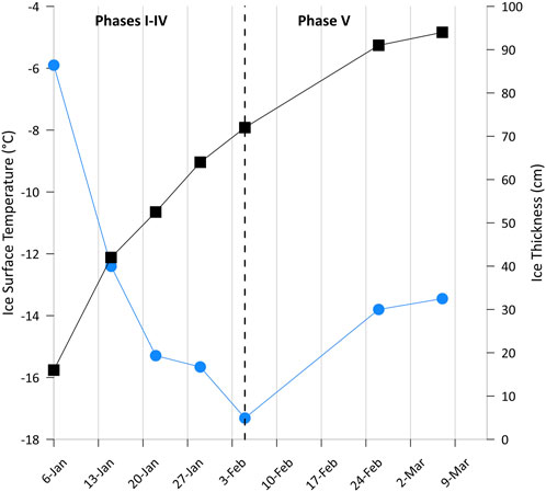
Figure 5. Decrease in ice surface temperature (blue dots) and increase in ice thickness (black squares) during the 2-month time series. Intense cooling resulted in a growth of more than 2/3 of the entire ice thickness in the first month.

4.1 Strong freeze initiating a methane pump

Lead opening in winter exposes the relatively warm underlying seawater to the cold air, resulting in rapid ice formation and growth by heat loss to the atmosphere. Strong brine entrapment affected by fast freeze causes high bulk salinities within the newly formed lead ice (Perovich and Gow, 1996). Indeed, we detected bulk surface salinities higher than those in FYI grown at the same time on this floe (Figure 6; Angelopoulos et al., 2022). A fast freeze favors upward brine expulsion to the surface ice layer (Notz and Worster, 2009). Pronounced half-C-shaped profiles of bulk salinity confirmed this upward-directed brine transport (Figures 3, 6). Exposing the highest-saline layer to the cold ice surface provoked counterintuitive physical properties: despite an ongoing strong freeze, the newly formed lead ice remained permeable for longer than 2 weeks (Figures 3, 4). Considering permeable ice as an open system (Golden et al., 2007), newly formed lead ice favors gas exchange coupled with brine migration between both interfaces, that is, to the atmosphere and ocean during that period.

Figure 6

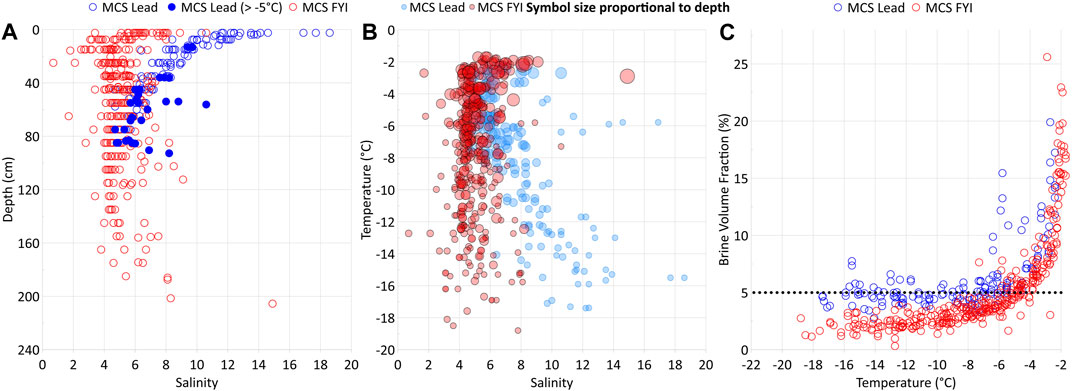
Figure 6. Salinity versus ice depth (A), temperature versus salinity (B), and brine volume fraction (BVF) versus temperature (C) in lead ice (blue dots) compared to first-year ice (red dots) from the main coring site (MCS FYI) in the Central Observatory during the MOSAiC drift expedition (locations see Figure 1). Salinities and BVF in lead ice grown in winter were generally higher than in FYI that developed on the same floe in early autumn. Lead ice remained completely permeable for more than 2 weeks.

In addition to affecting the physical properties, strong cooling also influenced the chemical properties, increasing the methane solubility at the ice surface and promoting in-gassing from the atmosphere (Figure 2). An eventual strong freeze induced a pronounced shift in the MSC-II in permeable lead ice compared to the MSC in seawater underneath. More precisely, accounting for the cooling of migrating brine to approximately −6°C causes an increase in MSC-II by approximately 20% related to the MSC of seawater (Figure 2). Therefore, seawater saturated with methane should induce an undersaturation related to MSC-II when the uptake of dissolved marine methane in permeable lead ice occurs. However, we observed methane saturation relative to MSC-II in lead ice, while methane was supersaturated relative to MSC in seawater. Consequently, the increase in solubility in permeable lead ice induced a solubility pump transporting methane downward through lead ice. Uptake at the ice surface might occur directly by dissolution of gaseous atmospheric methane or via an intermediate step, that is, indirectly by re-dissolution of methane previously released from high-saline frost flowers.

Cooling to −12°C further increased MSC-II (Figure 2), promoting continued dissolution of gaseous methane at the lead ice–air interface but also causing squeezing and subsequent gravity brine drainage. The “squeezing” caused a loss of methane by brine rejection, shown by the reduced concentration compared to the former phase at the lead ice surface. The interaction of the two processes initiated an incipient top-down transport of dissolved methane through the more than 30-cm-thick permeable lead ice layer (Figure 4). The ongoing uptake at the surface partly counterbalanced the loss by brine drainage and initiated a brief steady state period reflected in linear concentration and solubility gradients (Figures 3, 4). However, this period ceased before the end of Phase II. The convex-shaped concentration gradient pointed to an interrupted downward transport when the bottom layer grew.

Finally, cooling to −16°C resulted in the formation of a subsurface impermeable layer (SSIL), while the surface layer remained permeable due to the slightly higher bulk salinity. The SSIL separated the formerly complete permeable lead ice into an upper and lower permeable layer, interrupted the top-down brine drainage, and stopped the methane pump (Figures 3, 4). In impermeable ice, brine movement stops, but the brine is stored in isolated pockets (Golden et al., 2007; Crabeck et al., 2019). Hence, the formation of the SSIL caused a temporal offset in terms of methane stored in lead ice. While the SSIL preserves “frozen-in relicts” of earlier phases of ice formation, the permeable top and bottom layers mirror the impact of ongoing exchange at the interfaces between the ice surface and atmosphere on the one side and seawater on the other side. Indeed, methane uptake at the permeable top layer proceeded as cooling continued. Because the SSIL from that point on inhibited the downward transport, a methane excess on top of the SSIL developed (Figures 3, 4). By comparison, underneath the SSIL, methane loss by brine discharge continued from the permeable bottom layer to seawater. As uptake at the air–ice interface and loss at the ice–ocean interface took place contemporaneously, the concentration profiles changed from linear to half-C-shaped. This shift in gradients clearly assigned counter-rotating methane pathways when lead ice started to convert from completely permeable to partly impermeable (Figures 3, 4).

4.2 The shift from half-C- to C-shaped methane profiles

After a month, cooling at the surface ceased, disrupting the increase in solubility, and therefore, methane uptake at the air–ice interface stopped. At the same time, the lead ice surface became impermeable, enclosing the methane excess formed in the first month in disconnected brine pockets (Figures 3, 4). By comparison, cooling slowed but continued in subsurface lead ice. Consequently, the thicknesses of both the SSIL and the permeable bottom layer still increased, but brine release from the permeable layer weakened, as shown by the low Rayleigh numbers (Figure 3). The restricted brine release also reduced the loss of methane. Due to the gradient between MSC in seawater and MSC-II in open brine channels, methane replenishment from seawater into the highly permeable bottom layer started to occur at this point (Figures 2, 4). Accordingly, the former half-C-shaped concentration profiles developed toward rather C-shaped concentration profiles during the fifth and last phase, that is, the second month (Figure 4). Remarkably, this shift reflects how the strong freeze during the first month shaped the concentration profiles compared to the second month when mainly ice growth shaped the profiles, that is, either brine/methane release or ice growth/methane uptake dominated.

4.3 Isotopic fractionation effects during a strong freeze

While surface seawater was saturated to just slightly supersaturated, the δ¹³C–CH₄ ratios in seawater clearly deviated from the atmospheric equilibrium. Based on the atmospheric background of −47.5‰ (White et al., 2018) and taking into account up to 1‰ ¹³C-enrichment in seawater by kinetic isotopic fractionation (KIF) at the water–air interface (Knox et al., 1992; Happell et al., 1995), the δ¹³C–CH₄ ratio in surface seawater equilibrated with the atmosphere results in −46.5‰ VPDB. However, the δ¹³C–CH₄ ratio in seawater deviated by 8‰–10‰ ¹³C-enrichment from the atmospheric equilibrium value during the winter study. Remarkably, this pronounced shift even exceeded up to 5‰ of the ¹³C-enrichment detected during the melt season in this area (Damm et al., 2015; Verdugo et al., 2021). Seasonally altering δ¹³C–CH₄ ratios in seawater points to impacts of the sea ice life cycle on the marine methane pool by KIF effects. KIF effects are caused by the higher binding energy of the heavier isotopic molecule (¹³C), resulting in a lower mobility than the lighter isotopic molecule (¹²C) (Mook, 1994). Consequently, seasonal variations in δ¹³C–CH₄ ratios reveal a shift in the relative abundance of the ¹²C and ¹³C isotopes obviously related to melting and freezing processes.

Indeed, a ¹³C-depletion by at least 2‰ in newly formed lead ice related to the methane pool in seawater points to a higher abundance of the lighter (¹²C) isotope when marine methane became enclosed in brine (Figure 7). The ¹³C-depletion evidently strengthened when brine discharge occurred, as shown by the shift in δ¹³C–CH₄ ratios between newly formed and older lead ice (Figure 7). As occurring in the opposite direction than uptake, gravity favored the higher abundance of the heavier (¹³C) isotope on its way back to seawater, reinforcing on one side ¹³C-depletion in brine-methane and on the other side ¹³C-enrichment in marine methane.

Figure 7

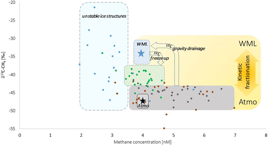
Figure 7. δ¹³C–CH₄ ratios related to methane concentration in newly formed lead ice (green dots) and lead ice from the time series (first and second month: brown and gray dots, respectively). The blue star in the blue field represents the range in surface seawater, that is, the winter mixed layer (WML), and the black star represents the atmospheric background. Freeze up and brine discharge induced shifts in δ¹³C–CH₄ ratios between methane dissolved in seawater and brine. Seawater was saturated to slightly supersaturated with methane, while the δ¹³C–CH₄ ratio in seawater was clearly enriched in ¹³C compared to the atmospheric background signature. This pattern points to gravity-triggered brine drainage as the main pathway for losing methane from lead ice. Note: The analyses of δ¹³C–CH₄ ratios might be influenced by the low concentrations in frost flowers (unstable ice structures; blue dots), finally contributing to the large variations in δ¹³C–CH₄ ratios.

Figure 8

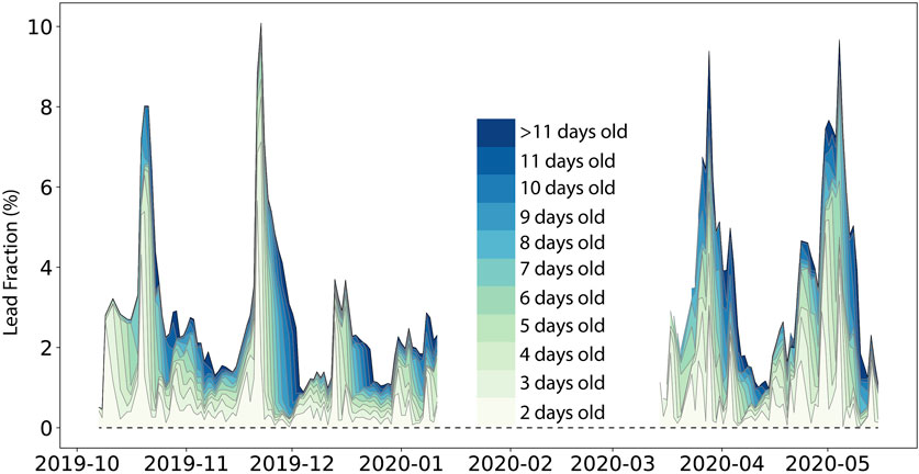
Figure 8. Lead fractions averaged in a circle with a 10 km radius around the RV Polarstern during the MOSAiC drift from 7 Oct 2019 to 15 May 2020. Colors indicate the percentage of leads of different ages between 2 days and > 11 days.

At the ice–air interface, methane dissolution induced by the solubility pump also contributed to δ¹³C–CH₄ ratio shifts in lead ice. Caused by differences in the molecular transfer rates of the lighter and heavier isotope (Mook, 1994), dissolution initiates a shift toward a ¹³C-enrichment in the relative abundance of the ¹²C and ¹³C isotopes, ultimately weakening the ¹³C-depletion in lead ice formerly induced by the KIF effect during ice formation. Consequently, because brine drainage and dissolution take place simultaneously and both processes partly counterbalance each other, δ¹³C–CH₄ ratios just vary less in aging lead ice.

4.4 Fast phase changes in frost flowers

Ice growth under winter conditions results in highly saline surface skim, often additionally covered by frost flowers. Frost flowers frequently develop at the surface of new sea ice, especially when the temperature gradient between surface ice and the overlaying atmosphere is large, and wind speeds are low. Initially, frost flowers are frozen freshwater, as they grow from the vapor phase, but the ice crystals wick up the brine from the surface of the sea ice, producing salinities of up to 180 PSU (Perovich and Richter-Menge, 1994; Domine et al., 2005). Their crystal-shaped configuration tends to provide a high total surface area of up to 1000 m² of ice surface (Domine et al., 2002), suggesting that frost flowers are sites for enhanced exchanges and chemical reactions (Rankin et al., 2002). These circumstances might also induce fast but pronounced shifts in the methane solubility capacity at the ice surface. Consequently, lead ice covered by frost flowers is a favored environment for phase changes between gaseous and dissolved methane. However, in opposition to the one-way direction of phase changes due to temperature decrease, the high variability in salinity at the ice surface during the life cycle of frost flowers enables phase changes in both directions. While low salinities in freshly formed frost flowers favor the dissolution of gaseous methane, increasing salinity induces a backward phase change, that is, a shift from dissolved to gaseous methane despite strong freezing. Large variations in δ¹³C–CH₄ ratios in frost flowers compared to those in lead ice potentially might refer to pronounced KIF effects by phase changes (Figure 7). However, we cannot exclude that the low concentrations affected the analyses of the δ¹³C–CH₄ ratios, finally inducing the large variations in δ¹³C–CH₄ ratios. To prove the proposed processes, in situ studies on frost flowers are required in the future.

4.5 Lead ice fraction in the new Arctic—an outlook

To estimate the Arctic-wide relevance of methane uptake at the ice surface on newly formed lead ice, we upscale our results with satellite observations of leads during MOSAiC. We use lead observations based on divergence previously presented in von Albedyll et al. (2023). With this dataset, we analyze the aerial coverage and lifetime of up to 10-day-old leads in a circle with a 10 km radius around MOSAiC and compare the results to circles with radii of 50 km, 100 km, and 150 km.

The mean aerial fraction (10-km scale) of up to 10-day-old leads was 3.2%, with a maximum of 10% (Figure 8). On 50% of the days, at least 2.5% of the area was covered by leads. Consequently, thin lead ice was an abundant feature of the sea ice cover. As shown above, the physical and chemical properties of up to 10–14-day-old lead ice mostly favored methane uptake at the lead ice surface. Von Albedyll et al. (2023) also showed that most of the leads during MOSAiC were short-lived (Figure 8). The median lifetime of leads was only 3 days, while only 2% of all leads did not close within 11 days. Thus, most of the leads during MOSAiC were an open system between the atmosphere and the ocean until an impermeable subsurface layer formed after this period.

The mean lead fractions from the MOSAiC expeditions on the 10 km scale (3.2%) are representative of the larger (50 km, 100 km, and 150 km) surroundings with a lead fraction of 3.1%–3.2%. However, some spatial lead dynamics differences emerge when the time series data are compared on a daily basis, resulting in a Pearson correlation coefficient of R = 0.6–0.7 (not shown).

Analyzing datasets from different Arctic regions, other studies found similar average lead fractions and maximum lifetimes of leads (Wadhams, 2000; Reiser et al., 2020; Hutter et al., 2023). Thus, we consider our estimates of lead aerial fraction and lifetime representative for a larger region and time beyond the drift of MOSAiC. Consequently, uptake at the ice surface and pumping through thin lead ice is a significant yet unconsidered methane pathway in the Arctic. The relevance of this process may even increase when the Arctic fully transitions into a seasonally ice-covered ocean where leads may be more abundant than in the central ice pack (Kwok et al., 2006).

5 Conclusion

Estimates of the occurrence and frequency of young lead ice from satellite observations highlight the relevance of this ice type in a warming Arctic. Our process study of rapid lead ice growth conditions and properties in winter has identified some previously unconsidered methane pathways between sea ice, ocean, and atmosphere.

1) Fast brine entrapment can keep newly formed lead ice completely permeable for up to 2 weeks. During that period, the imbalanced effect of temperature decrease and salinity increase on the methane solubility capacity leads to physical conditions that support a top-down methane pump. The decrease in surface temperature triggers how long methane uptake can occur.

2) The time variable onset of impermeable conditions in the ice column results in vertical methane gradients that reflect concurrent ongoing transport processes and storage of methane in “frozen-in” zones. Identifying temporal delays of those freeze effects on methane gradients in ice cores will contribute to an improved interpretation of the methane “history” stored in single, “snapshot” ice cores taken later in the season.

3) We show for the first time that freeze strongly affects the δ¹³C–CH₄ ratios in seawater and newly formed lead ice, resulting, on the one hand, in seasonal shifts of the isotopic signature in the marine methane pool and, on the other hand, in a clear enrichment of the ¹³C isotope of marine methane compared to the atmospheric background signature.

4) The revealed methane pathways highlight an intense circulation of methane between seawater and sea ice during freeze. In comparison, the air–ice interaction is restricted to phases when physical conditions enable air-to-ice in-gassing.

Data availability statement

The raw data presented in the study are available in PANGAEA. Further inquiries can be directed to the corresponding author.

Author contributions

ED: conceptualization, data curation, formal analysis, funding acquisition, investigation, methodology, project administration, resources, visualization, and writing–original draft. ST: conceptualization, formal analysis, funding acquisition, methodology, and writing–original draft. MA: data curation, investigation, methodology, visualization, writing–review and editing, and formal analysis. LV: conceptualization, methodology, visualization, and writing–original draft. AR: data curation, validation, and writing–review and editing. CH: funding acquisition, validation and writing–review and editing.

Funding

The author(s) declare that financial support was received for the research, authorship, and/or publication of this article. The work was funded by the German Federal Ministry for Education and Research (BMBF) through financing the Alfreds Wegener-Institut Helmholtz Zentrum für Polar-und Meeresforschung (AWI) and the RV Polarstern expedition PS122 under grant N-2014-H-060_Dethloff and the AWI through its project: AWI_BGC. The work carried out and data used in this manuscript were produced as part of the International Multidisciplinary Drifting Observatory for the Study of the Arctic Climate (MOSAiC) with the tag MOSAiC20192020. ST was supported by DFG—priority program SPP 1158 by the following grant: TH744/7-1.

Acknowledgments

We thank all persons involved in the expedition of the Research Vessel RV Polarstern during MOSAiC in 2019–2020 (AWI_PS122_00) as listed in Nixdorf et al. (2021). We highly thank all the participants for the fieldwork in the Central Observatory, especially Patric Simones Pereira, Adela Dumitrescu, Torsten Sachs, and Hans Werner Jacobi, who contributed to sampling thin new ice and frost flowers in the field.

Conflict of interest

The authors declare that the research was conducted in the absence of any commercial or financial relationships that could be construed as a potential conflict of interest.

Publisher’s note

All claims expressed in this article are solely those of the authors and do not necessarily represent those of their affiliated organizations, or those of the publisher, the editors, and the reviewers. Any product that may be evaluated in this article, or claim that may be made by its manufacturer, is not guaranteed or endorsed by the publisher.

Supplementary material

The Supplementary Material for this article can be found online at: https://www.frontiersin.org/articles/10.3389/feart.2024.1338246/full#supplementary-material

References

Angelopoulos, M., Damm, E., Simões Pereira, P., Abrahamsson, K., Bauch, D., Bowman, J., et al. (2022). Deciphering the properties of different arctic ice types during the growth phase of MOSAiC: implications for future studies on gas pathways. Front. Earth Sci. 10. doi:10.3389/feart.2022.864523

CrossRef Full Text | Google Scholar

Assur, A. (1960). Composition of sea ice and its tensile strength, 44. Wilmette, Illinois: US Army Snow, Ice and Permafrost Research Establishment.

Google Scholar

Bartels-Rausch, T., Kong, X., Orlando, F., Artiglia, L., Waldner, A., Huthwelker, T., et al. (2021). Interfacial supercooling and the precipitation of hydrohalite in frozen NaCl solutions as seen by X-ray absorption spectroscopy. Cryosphere 15, 2001–2020. doi:10.5194/tc-15-2001-2021

CrossRef Full Text | Google Scholar

Boutin, G., Ólason, E., Rampal, P., Regan, H., Lique, C., Talandier, C., et al. (2023). Arctic sea ice mass balance in a new coupled ice–ocean model using a brittle rheology framework. Cryosphere 17, 617–638. doi:10.5194/tc-17-617-2023

CrossRef Full Text | Google Scholar

Cox, G. F. N., and Weeks, W. F. (1983). Equations for determining the gas and brine volumes in sea-ice samples. J. Glaciol. 29, 306–316. doi:10.1017/s0022143000008364

CrossRef Full Text | Google Scholar

Crabeck, O., Galley, R. J., Mercury, L., Delille, B., Tison, J. L., and Rysgaard, S. (2019). Evidence of freezing pressure in sea ice discrete brine inclusions and its impact on aqueous-gaseous equilibrium. J. Geophys. Res. Oceans 124, 1660–1678. doi:10.1029/2018JC014597

CrossRef Full Text | Google Scholar

Damm, E., Bauch, D., Krumpen, T., Rabe, B., Korhonen, M., Vinogradova, E., et al. (2018). The transpolar drift conveys methane from the siberian shelf to the central Arctic Ocean. Sci. Rep. 8, 4515. doi:10.1038/s41598-018-22801-z

PubMed Abstract | CrossRef Full Text | Google Scholar

Damm, E., Helmke, E., Thoms, S., Schauer, U., Nöthig, E., Bakker, K., et al. (2010). Methane production in aerobic oligotrophic surface water in the central Arctic Ocean. Biogeosciences 876, 1099–1108. doi:10.5194/bg-7-1099-2010

CrossRef Full Text | Google Scholar

Damm, E., Rudels, B., Schauer, U., Mau, S., and Dieckmann, G. (2015). Methane excess in arctic surface water- triggered by sea ice formation and melting. Sci. Rep. 5, 16179. doi:10.1038/srep16179

PubMed Abstract | CrossRef Full Text | Google Scholar

Domine, F., Cabanes, A., and Legagneux, L. (2002). Structure, microphysics, and surface area of the Arctic snowpack near Alert during the ALERT 2000 campaign. Atmos. Environ. 36, 2753–2765. doi:10.1016/s1352-2310(02)00108-5

CrossRef Full Text | Google Scholar

Domine, F., Taillandier, A. S., Simpson, W. R., and Severin, K. (2005). Specific surface area, density and microstructure of frost flowers. Geophys. Res. Lett. 32, L13502. doi:10.1029/2005GL023245

CrossRef Full Text | Google Scholar

Fukusako, S. (1990). Thermophysical properties of ice, snow, and sea ice. Int. J. Thermophys. 11, 353–372. doi:10.1007/BF01133567

CrossRef Full Text | Google Scholar

Golden, K. M., Eicken, H., Heaton, A. L., Miner, J., Pringle, D. J., and Zhu, J. (2007). Thermal evolution of permeability and microstructure in sea ice. Geophys. Res. Lett. 34. doi:10.1029/2007GL030447

CrossRef Full Text | Google Scholar

Gourdal, M., Crabeck, O., Lizotte, M., Galindo, V., Gosselin, M., Babin, M., et al. (2019). Upward transport of bottom-ice dimethyl sulfide during advanced melting of arctic first-year sea ice. Elem. Sci. Anthr. 7. doi:10.1525/elementa.370

CrossRef Full Text | Google Scholar

Haas, C., Hoppmann, M., Tippenhauer, S., and Rohardt, G. (2021). Continuous thermosalinograph oceanography along RV POLARSTERN cruise track PS122/2. PANGAEA. doi:10.1594/PANGAEA.930024

CrossRef Full Text | Google Scholar

Happell, J. D., Chanton, J. P., and Showers, W. J. (1995). Methane transfer across the water-air interface in stagnant wooded swamps of Florida: evaluation of mass-transfer coefficients and isotropic fractionation. Limnol. Oceanogr. 40 (2), 290–298. doi:10.4319/lo.1995.40.2.0290

CrossRef Full Text | Google Scholar

Hutter, N., Hendricks, S., Jutila, A., Ricker, R., von Albedyll, L., Haas, C., et al. (2023). Digital elevation models of the sea-ice surface from airborne laser scanning during MOSAiC. Sci. Data 10, 729. doi:10.1038/s41597-023-02565-6

PubMed Abstract | CrossRef Full Text | Google Scholar

Katlein, C., Mohrholz, V., Sheikin, I., Itkin, P., Divine, D. V., Stroeve, J., et al. (2020). Platelet ice under arctic pack ice in winter. Geophys. Res. Lett. 47, e2020GL088898. doi:10.1029/2020GL088898

CrossRef Full Text | Google Scholar

Kiditis, V., Upstill-Goddard, R. C., and Anderson, L. (2010). Methane and nitrous oxide in surface water along the north-west passage, Arctic Ocean. Mar. Chem. 121 (issue 1-4), 80–86. doi:10.1016/j.marchem.2010.03.006

CrossRef Full Text | Google Scholar

Knox, M., Quay, P. D., and Wilbur, D. (1992). Kinetic isotopic fractionation during air-water gas transfer of 0₂, N₂, CH₄, and H₂. J. Geophys. Res. 97 (C12), 335–343.

CrossRef Full Text | Google Scholar

Kort, E. A., Wofsy, S. C., Daube, B. C., Diao, M., Elkins, J. W., Gao, R. S., et al. (2012). Atmospheric observations of Arctic Ocean methane emissions up to 82° north. Nat. Geosci. 5, 318–321. doi:10.1038/ngeo1452

CrossRef Full Text | Google Scholar

Krumpen, T., Belter, H. J., Boetius, A., Damm, E., Haas, C., Hendricks, S., et al. (2019). Arctic warming interrupts the Transpolar Drift and affects long-range transport of sea ice and ice-rafted matter. Sci. Rep. 9, 5459. doi:10.1038/s41598-019-41456-y

PubMed Abstract | CrossRef Full Text | Google Scholar

Kwok, R. (2006). Contrasts in sea ice deformation and production in the Arctic seasonal and perennial ice zones. J. Geophys. Res. 111, C11S22. doi:10.1029/2005jc003246

CrossRef Full Text | Google Scholar

Kwok, R. (2018). Arctic sea ice thickness, volume, and multiyear ice coverage: losses and coupled variability (1958–2018). Environ. Res. Lett. 13 (10), 105005. doi:10.1088/1748-9326/aae3ec

CrossRef Full Text | Google Scholar

Li, Y., Fichot, C. G., Geng, L., Scarratt, M. G., and Xie, H. (2020). The contribution of methane photoproduction to the oceanic methane paradox. Geophys. Res. Lett. 47. doi:10.1029/2020GL088362

CrossRef Full Text | Google Scholar

Manning, C. C. M., Zheng, Z., Fenwick, L., McCulloch, R. D., Damm, E., Izett, R. W., et al. (2022). Interannual variability in methane and nitrous oxide concentrations and sea-air fluxes across the north American Arctic Ocean (2015–2019). Glob. Biogeochem. Cycles 36 (4), e2021GB007185. doi:10.1029/2021GB007185

CrossRef Full Text | Google Scholar

Mook, W. (1994). Principles of isotope hydrology. Introductory course on Isotope Hydrology. Dep. Hydrogeol. Geogr. Hydrol. VU Amsterdam, Amsterdam.

Google Scholar

Nicolaus, M., Perovich, D. K., Spreen, G., Granskog, M. A., Albedyll, L., Angelopoulos, M., et al. (2022). Overview of the MOSAiC expedition- Snow and sea ice. Elem. Sci. Anthropocene 10 (1). doi:10.1525/elementa.2021.000046

CrossRef Full Text | Google Scholar

Nixdorf, U., Dethloff, K., Rex, M., Shupe, M., Sommerfeld, A., Perovich, D. K., et al. (2021). MOSAiC extended acknowledgement. doi:10.5281/zenodo.5179739

CrossRef Full Text | Google Scholar

Notz, D. (2005). Thermodynamic and fluid-dynamical processes in sea ice. University of Cambridge. Ph. D. thesis.

Google Scholar

Notz, D., and Worster, M. G. (2009). Desalination processes of sea ice revisited. J. Geophys. Res. 114. doi:10.1029/2008JC004885

CrossRef Full Text | Google Scholar

Ólason, E., Rampal, P., and Dansereau, V. (2021). On the statistical properties of sea-ice lead fraction and heat fluxes in the Arctic. Cryosphere 15, 1053–1064. doi:10.5194/tc-15-1053-2021

CrossRef Full Text | Google Scholar

Perovich, D. K., and Gow, A. J. (1996). A quantitative description of sea ice inclusions. J. Geophys. Res. 101 (C8), 18327–18343. doi:10.1029/96jc01688

CrossRef Full Text | Google Scholar

Perovich, D. K., and Richter-Menge, J. A. (1994). Surface characteristics of lead ice. J. Geophys. Res. 99 (C8), 16341–16350. 16,341-16,350. doi:10.1029/94jc01194

CrossRef Full Text | Google Scholar

Pohlmann, J. W., Casso, M., Magen, C., and Bergeron, E. (2021). Discrete sample introduction Module for quantitative and isotopic analysis of methane and other gases by cavity ring-down spectroscopy. Environ. Sci. Technol. 55 (17), 12066–12074. 12,066-12,074. doi:10.1021/acs.est.1c01386

PubMed Abstract | CrossRef Full Text | Google Scholar

Rabe, B., Heuzé, C., Regnery, J., Aksenov, Y., Allerholt, J., Athanase, M., et al. (2022). Overview of the MOSAiC expedition- Physical oceanography. Elem. Sci. Anthropocene 10 (1). doi:10.1525/elementa.2021.00062

CrossRef Full Text | Google Scholar

Rankin, A. M., Wolff, E. W., and Martin, S. (2002). Frost flowers: implications for tropospheric chemistry and ice core interpretation. J. Geophys. Res. 107 (D23), 4683. doi:10.1029/2002JD002492

CrossRef Full Text | Google Scholar

Rantanen, M., Karpechko, A. Y., Lipponen, A., Nordling, K., Hyvärinen, O., Ruosteenoja, K., et al. (2022). The Arctic has warmed nearly four times faster than the globe since 1979. Commun. Earth Environ. 3, 168. doi:10.1038/s43247-022-00498-3

CrossRef Full Text | Google Scholar

Reiser, F., Willmes, S., and Heinemann, G. (2020). A new algorithm for daily sea ice lead identification in the arctic and antarctic winter from thermal-infrared satellite imagery. Remote Sens. 12, 1957. doi:10.3390/rs12121957

CrossRef Full Text | Google Scholar

Rella, C. W., Hoffnagle, J., He, Y., and Tajima, S. (2015). Local- and regional-scale measurements of CH&amp;lt;sub&amp;gt;4&amp;lt;/sub&amp;gt;, δ<sup&amp;gt;13&amp;lt;/sup&amp;gt;CH&amp;lt;sub&amp;gt;4&amp;lt;/sub&amp;gt;, and C&amp;lt;sub&amp;gt;2&amp;lt;/sub&amp;gt;H&amp;lt;sub&amp;gt;6&amp;lt;/sub&amp;gt; in the Uintah Basin using a mobile stable isotope analyzer. Atmos. Meas. Tech. 8, 4539–4559. doi:10.5194/amt-8-4539-2015

CrossRef Full Text | Google Scholar

Rosenfeld, D., and Woodley, W. (2000). Deep convective clouds with sustained supercooled liquid water down to -37.5 °C. Nature 405 (6785), 440–442. doi:10.1038/35013030

PubMed Abstract | CrossRef Full Text | Google Scholar

Serreze, M. C., and Barry, R. G. (2011). Processes and impacts of Arctic amplification: a research synthesis. Glob. Planet. Change 77, 85–96. doi:10.1016/j.gloplacha.2011.03.004

CrossRef Full Text | Google Scholar

Shupe, M. D., Rex, M., Blomquist, B., Persson, P. O. G., Schmale, J., Uttal, T., et al. (2022). Overview of the MOSAiC expedition—atmosphere. Elem. Sci. Anthropocene 10 (1). doi:10.1525/elementa.2021.00060

CrossRef Full Text | Google Scholar

Silyakova, A., Nomura, D., Kotovich, M., Fransson, A., Delille, B., Chierici, M., et al. (2022). Methane release from open leads and new ice following an Arctic winter storm event. Pol. Sci. 33, 100874. doi:10.1016/j.polar.2022.100874

CrossRef Full Text | Google Scholar

Steiner, N. S., Lee, W. G., and Christian, J. R. (2013). Enhanced gas fluxes in small sea ice leads and cracks: effects on CO2 exchange and ocean acidification. J. Geophys. Res. Oceans 118, 1195–1205. doi:10.1002/jgrc.20100

CrossRef Full Text | Google Scholar

Stroeve, J., and Notz, D. (2018). Changing state of Arctic sea ice across all seasons. Environ. Res. Lett. 13 (10), 103001. doi:10.1088/1748-9326/aade56

CrossRef Full Text | Google Scholar

Sumata, H., de Steur, L., Divine, D. V., Granskog, M. A., and Gerland, S. (2023). Regime shift in Arctic ocean sea ice thickness. Nature 615, 443–449. doi:10.1038/s41586-022-05686-x

PubMed Abstract | CrossRef Full Text | Google Scholar

Tison, J. L., Delille, B., and Papadimitriou, S. (2017). “Gases in sea ice,” in Gases in sea ice (Chichester, UK: John Wiley and Sons), 433–471. Chap. 18. doi:10.1002/9781118778371.ch18

CrossRef Full Text | Google Scholar

Torsvik, T. (2023). Modeling influence of sea ice on gas exchanges between atmosphere and ocean in a global. Earth Syst. Model. Assembly 2023. doi:10.5194/egusphere-egu23-9684EGU

CrossRef Full Text | Google Scholar

Uhlig, C., Kirkpatrick, J. B., D’Hondt, S., and Loose, B. (2018). Methane-oxidizing seawater microbial communities from an Arctic shelf. Biogeosciences 15, 3311–3329. doi:10.5194/bg-15-3311-2018

CrossRef Full Text | Google Scholar

Uhlig, C., and Loose, B. (2017). Using stable isotopes and gas concentrations for independent constraints on microbial methane oxidation at Arctic Ocean temperatures. Limnol. Oceanogr. Methods 15, 737–751. doi:10.1002/lom3.10199

CrossRef Full Text | Google Scholar

Valentine, D. L. (2002). Biogeochemistry and microbial ecology of methane oxidation in anoxic environments: a review. Antonie Leeuwenhoek 81, 271–282. doi:10.1023/a:1020587206351

PubMed Abstract | CrossRef Full Text | Google Scholar

Verdugo, J., Damm, E., and Nikolopoulos, A. (2021). Methane cycling within sea ice; results from drifting ice during late spring, north of svalbard. Cryosphere 15, 2701–2717. doi:10.5194/tc-15-2701-2021

CrossRef Full Text | Google Scholar

Vinogradova, E., Damm, E., Pnyushkov, A. V., Krumpen, T., and Ivanov, V. (2022). Shelf-sourced methane in surface seawater at the eurasian continental slope (Arctic Ocean). Front. Envir. Sci. 8, 811375. doi:10.3389/fenvs.2022.811375

CrossRef Full Text | Google Scholar

Von Albedyll, L., Hendricks, S., Grodofzig, R., Krumpen, T., Arndt, S., Belter, H. J., et al. (2022). Thermodynamic and dynamic contributions to seasonal Arctic sea ice thickness distributions from airborne observations. Elem. Sci. Anthropocene 10. doi:10.1525/elementa.2021.00074

CrossRef Full Text | Google Scholar

Von Albedyll, L., Hendricks, S., Hutter, N., Murashkin, D., Kaleschke, L., Willmes, S., et al. (2023). Lead fractions from SAR-derived sea ice divergence during MOSAiC. Cryosphere (Disc,). doi:10.5194/tc-2023-123

CrossRef Full Text | Google Scholar

Wadhams, P. (2000). Ice in the ocean. London (UK): Gordon and Breach Science Publishers. 90-5699-296-1.

Google Scholar

Weeks, W. F., and Ackley, F. S. (1986). “The growth, structure and properties of sea ice,” in Geophysics of sea ice. Editor N. Untersteiner (London: Plenum press), 9–164. (NATO ASI series, B: Physics 146).

CrossRef Full Text | Google Scholar

White, J., Vaughn, B. H., and Michel, S. (2018). University of Colorado, institute of arctic and alpine research (INSTAAR), stable isotopic composition of atmospheric methane (13C) from the NOAA ESRL carbon cycle cooperative global air sampling network, 1998–2017 (version 2018-09-24). Available at: ftp://aftp.cmdl.noaa.gov/data/trace_gases/ch4c13/flask/.

Google Scholar

Wiesenburg, D. A., and Guinasso, N. L. (1979). Equilibrium solubilities of methane, carbon monoxide, and hydrogen in water and seawater. J. Chem. Eng. Data 24, 356–360. doi:10.1021/je60083a006

CrossRef Full Text | Google Scholar

Wilchinsky, A. V., Heorton, H. D. B. S., Feltham, D. L., and Holland, P. R. (2015). Study of the impact of ice formation in leads upon the sea ice pack mass balance using a new frazil and grease ice parameterization. J. Phys. Oceanogr. 45, 2025–2047. doi:10.1175/jpo-d-14-0184.1

CrossRef Full Text | Google Scholar

Willmes, S., Heinemann, G., and Schnaase, F. (2023). Patterns of wintertime Arctic sea-ice leads and their relation to winds and ocean currents. Cryosphere 17, 3291–3308. doi:10.5194/tc-17-3291-2023

CrossRef Full Text | Google Scholar

Xin, He, Sun, L., Xie, Z., Huang, W., Long, N., Li, Z., et al. (2013). Sea ice in the Arctic Ocean: role of shielding and consumption of methane. Atmos. Environ. 67, 8–13. doi:10.1016/j.atmosenv.2012.10.029

CrossRef Full Text | Google Scholar

Zhang, F., Pang, X., Lei, R., Zhai, M., Zhao, X., and Cai, Q. (2021). Arctic sea ice motion change and response to atmospheric forcing between 1979 and 2019. Int. J. Climatol. 42, 1854–1876. doi:10.1002/joc.7340

CrossRef Full Text | Google Scholar

Zhou, J., Delille, B., Eicken, H., Vancoppenolle, M., Brabant, F., Carnat, G., et al. (2013). Physical and biogeochemical properties in landfast sea ice (barrow, Alaska): insights on brine and gas dynamics across seasons. J. Geophys. Res. Oceans 118, 3172–3189. doi:10.1002/jgrc.20232

CrossRef Full Text | Google Scholar

Zhou, J., Tison, J.-L., Carnat, G. N., Geilfus, X., and Delille, B. (2014). Physical controls on the storage of methane in landfast sea ice. Cryosphere 8, 1019–1029. doi:10.5194/tc-8-1019-2014

CrossRef Full Text | Google Scholar