Bayesian maximum entropy interpolation analysis for rapid assessment of seismic intensity using station and ground motion prediction equations

1 Introduction

Seismic intensity is the most intuitive parameter used to reflect the strength of ground motion and its influence. The United States (US) first released the ShakeMap system in 1999. US states have established a network with numerous stations; the system quickly obtains seismic ground motion parameters, such as peak ground acceleration (PGA), peak ground velocity (PGV), and peak ground displacement (PGD), at stations after an earthquake and an intensity distribution map is created by combining this instrument-based ground motion data with theoretical interpolation (multivariate normal (MVN)) results (Worden et al., 2010). Many early warning stations have also been deployed in Chinese Taiwan, and the seismic intensity rapid reporting system is mainly composed of a rapid reporting system (RSS) and an early warning system (EWS) (Kinoshita, 1998); this approach is older and more comprehensive than that employed in mainland China. At present, some scholars have developed rapid seismic intensity assessment methods based on real-time seismology (source rupture process) (Smith and Mooney, 2021), and these studies have explored rapid seismic intensity assessment methods and achieved fruitful results (Chen et al., 2022a; Chen et al., 2022b; Peng et al. 2023), which have been well applied in practical earthquake emergency response cases (Chen et al., 2022c). In addition to these methods, other seismic intensity assessment methods based on network surveys (Did You Feel It?) (Atkinson and Wald, 2007) and remote sensing information extraction (optical remote sensing, radar, interferometric synthetic aperture radar (InSAR) have been developed (Wang et al., 2015; Xiao et al., 2022; Guo et al., 2024). China is expected to build nationwide earthquake early warning stations in 2023. Although stations in the network are relatively abundant, the geographical distribution varies considerably, with most located in the southeastern coastal areas of China and the Qinghai-Tibet Plateau and on the Loess Plateau in western China (Wang et al., 2017; Peng et al., 2021). Using unevenly distributed seismic stations to combine existing knowledge to carry out postearthquake emergency response has quickly has become a pressing problem. This paper explores a spatial interpolation method based on existing station data combined with a seismic ground motion prediction equation (GMPE). Gehl used Bayesian networks (BNs) based on continuous Gaussian variables to predict the spatial distribution of ground motion parameters; this approach exploits the spatial distribution of intraevent and interevent errors in a ground motion prediction equation and can predict uncertain variables based on given observations, but BNs are computationally expensive (Gehl et al., 2017). The ShakeMap system uses the MVN distribution proposed by Worden for weighted interpolation, which is a way of combining stations with the GMPE and requires the selected data to be normally distributed. The Bayesian maximum entropy (BME) discussed in this paper does not require the data to be normally distributed and is more comprehensive regarding data availability.

Although classic geostatistics has matured, there are still some defects in the application process, such as the inability to use empirical data other than sampled data, the need for stationary assumptions or Gaussian assumptions; moreover, the use of the best linear unbiased estimate (BLUE) can cause the smoothing of predicted values (Christakos and Li, 1998). Given these defects, in the early 1990s, Christakos proposed a new concept of spatial valuation: the BME method (Christakos, 1990). The established BME-based geostatistical method adopts the Bayesian method in statistics and the concept of entropy in information theory to recognize and deal with spatiotemporal variables, which are an integral part of modern spatiotemporal geostatistics. The BME theory is rooted in the spatiotemporal random field model (S/TRF). This model expands upon the spatial random field (SRF) concept from classical geostatistics by incorporating the temporal dimension, conceptualizing natural processes as fields comprised of random variables across both space and time. After more than 10 years of development, the BME-based geostatistical method has been successfully applied in fields such as soil science, environmental science, and infectious diseases control (Douaik et al., 2005; Wibrin et al., 2006; Couliette et al., 2009; Yu et al., 2011). Compared with the traditional kriging interpolation method, the BME approach does not require assumptions about linear estimation, spatial homogeneity or a normal distribution and can integrate hard and soft data to improve the analysis accuracy. Christakos et al. (2004) constructed soft data based on the relationship between tropopause pressure and total ozone to predict the spatiotemporal distribution of total ozone in the US. They used the relatively accurate total ozone obtained by remote sensing satellites as hard data for BME analysis. Money et al. (2009) used site data as hard data and model estimations as soft data to conduct a spatiotemporal analysis of Escherichia coli concentrations in the Raritan River watershed in New Jersey, United States from 2000 to 2006, and their results showed that the BME analysis improved accuracy by 30%. The successful application of the BME method in various fields has confirmed that the BME method is reliable, and the most significant advantage is that the application of soft data is flexible.

The BME and ShakeMap algorithms are both based on probability density functions (PDFs). However, there is no apparent connection between the weighted interpolation approach used in the ShakeMap algorithm and the spatial correlation coefficient used in the BME method, which makes direct comparison of the two methods complicated. In this paper, the Wells empirical formula (Wells and Coppersmith, 1994) can be used to quickly obtain the GMPE results after an earthquake, and the predicted ground motion parameters can be obtained within a few minutes after the station data are obtained. The ground motion map produced by ShakeMap after an earthquake is the result of combining MVN and GMPE information. Similarly, the predicted seismic motion map in this article combines BME and GMPE data. However, it is worth noting that the use of GMPE in this article differs from that of ShakeMap. ShakeMap primarily relies on GMPE models from NGA-West2, such as CB2014 and BSSA 2014 (Boore et al., 2014; Campbell and Bozorgnia, 2014). These GMPE predictions are based on finite fault models, requiring many input parameters, including the fault layer’s dip angle, slip angle, width of fault rupture, earthquake magnitude, shortest fault distance, shortest fault projection distance, and more. In contrast, the Si model used in this article simplifies the process, requiring only three parameters: magnitude, shortest fault projection distance (Rjb), and Vs30. Therefore, the calculation parameters of ShakeMap with NGA-West 2 GMPE are more complex. In this article, the BME method uses a simplified GMPE (SI model), providing a faster and more direct calculation process for post-earthquake seismic intensity assessment. The combined GMPE method in this article is not as complex as the method in ShakeMap. This simplified method can quickly generate prediction results after earthquakes, and its prediction accuracy can be comparable to ShakeMap.

In this paper, Section 2 introduces the data sources and the modeling methods. In Section 3, the 2016 Kumamoto Mw7 earthquake in Japan, the 2019 California Mw7 earthquake in the US, and the 2023 Turkey Mw7.8 earthquake are selected as examples to show the application effect and accuracy of the proposed method. In Section 4, the reliability and applicable conditions of the proposed method are discussed. Finally, a summary of the research is provided in Section 5.

2 Materials and methods

2.1 Materials

Due to the difficulty obtaining strong ground motion data in many areas, the 2016 Kumamoto earthquake in Japan (hereinafter referred to as the Japan earthquake), the 2019 California earthquake in the US (hereinafter referred to as the US earthquake), and the 2023 Turkey Mw7.8 earthquake (hereinafter referred to as the Turkey earthquake), which occurred on 6 February 2023, are selected as the earthquake cases. The earthquake magnitudes, epicenter locations, and focal depths are all provided by ShakeMap. The isoseismals used in this paper are also provided by ShakeMap (Modified Mercalli Intensity (MMI)). Many scholars have established the relationship between the duration of strong ground motion acceleration, velocity, and displacement, as well as the MMI (Trifunac and Brady, 1975; Atkinson and Sonley, 2000; Worden et al., 2012). For the soft data, the formula released by Si in 1999 is used as the GMPE (Si and Midorikawa, 1999); it has been verified in many earthquake cases, and the results have been proven to be reliable and applicable (Chen et al., 2022b; Zhao et al., 2022; Kang et al., 2023; An et al., 2023; Peng et al., 2023; Chen et al., 2023; Zhou et al., 2024; Jia et al., 2024). The ground motion value mainly used in this article is the PGV. In order to achieve faster seismic intensity assessment, we performed linear field correction on PGV (PGA is usually non-linear field correction) (Chen et al., 2022b). Both GMPE and instrument records were calculated using PGV as the input value. Among them, the conversion from PGV to MMI is based on conversion relationship (Worden et al., 2012). PGV values recorded at the stations with strong ground motion data are used as the hard data (https://earthquake.usgs.gov/earthquakes/eventpage/us6000jllz/ShakeMap/stations). ArcGIS is used to extract the soft data, and finally, an intensity map is output to test the prediction results. The test data mainly uses the measured data by stations and the isoseismals downloaded from ShakeMap. The implementation of the BME method is mainly realized in SEKS-GUI software, which is based on the modern geostatistical theory proposed by Christakos in 1990 and demonstrated by examples (Christakos, 2000; Yu et al., 2007). The site amplification factor describes the amplification effect of seismic motion when geological conditions change. This is crucial for assessing the seismic risk of buildings and infrastructure, and can also be used to explain the changes in seismic intensity in geographic space. The amplification factor of different locations on the same site may be different, which can lead to differences in seismic intensity in different areas on the same site, and the site amplification factor is often related to Vs30 (Krinitzsky and Chang, 1988; Yaghmaei-Sabegh and Hassani, 2020). The Vs30 data used for field corrections are obtained from the US Geological Survey (https://earthquake.usgs.gov/data/vs30/). All seismic data are listed in Table 1.

Table 1

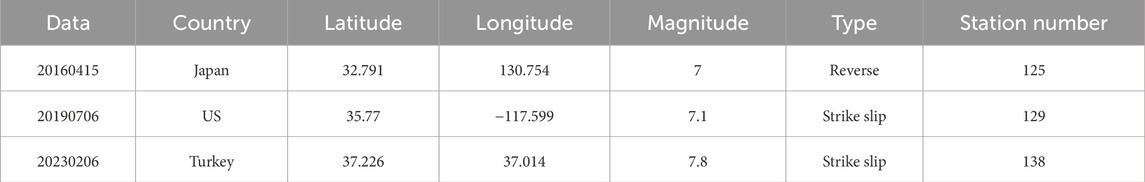
Table 1. The earthquake cases.

2.2 Methods

2.2.1 BME

2.2.1.1 BME analysis

In the BME method, the acquired information or knowledge is generally divided into two categories. One is called general knowledge G, which usually includes common sense, physical laws, scientific theories, and statistical data. The other is called specific knowledge S, which represents a specific phenomenon or thing, such as the hard data and soft data mentioned above. General knowledge G and specific knowledge S together form knowledge set K, that is, $\mathrm{K}=\mathrm{G}\cup \mathrm{S}$. The BME process is a logical reasoning process that considers the use of overall knowledge K and the way to use knowledge to solve problems, with three main stages: the prior stage, meta-prior stage, and posterior stage. In the prior stage, the principle of maximum entropy is used to find the prior PDF $f_G$, and thus, the maximum of G is close to the real value to the greatest extent possible. In the meta-prior stage, the form of specific knowledge S is converted, and in the posterior stage, $f_G$ and S are combined to update $f_G$ based on a generalized Bayesian formulation to obtain the posterior PDF $f_K$. The procedure is shown in Figure 1. If there are m spatiotemporal points in S/TRF, i.e., [$p_1···p_m$]^T, $m_h$ pieces of hard data, and $m_s$ pieces of soft data, then ${\mathrm{\chi }}_{data}=\left[{\mathrm{\chi }}_{hard},{\mathrm{\chi }}_{soft}\right]$, where ${\mathrm{\chi }}_{data}=\left[x_1···x_m\right]$^T, ${\mathrm{\chi }}_{hard}=\left[x_1···x_{mh}\right]$^T, and ${\mathrm{\chi }}_{soft}=\left[x_{m_h}···x_m\right]$^T are all data, hard data, and soft data, respectively. ${\mathrm{\chi }}_k$ represents the predicted value of the point to be estimated, $f_G\left({\chi }_{map}\right)$ is the prior PDF of ${\chi }_{map}$ based on G, and $f_K\left({\chi }_k\right)$ is the posterior PDF of ${\chi }_k$ based on K. The corresponding formulas are as follows:

${\mathrm{P}}_{\mathrm{x}}\left(\mathrm{\chi }\right)=\text{Prob}\left[{\mathrm{\chi }}_1<{\mathrm{x}}_1<\mathrm{d}{\mathrm{\chi }}_1,...,{\mathrm{\chi }}_{\mathrm{m}}<{\mathrm{x}}_{\mathrm{m}}<\mathrm{d}{\mathrm{\chi }}_{\mathrm{m}}\right]={\mathrm{f}}_{\mathrm{x}}\left(\mathrm{\chi }\right){\mathrm{d}}_{\mathrm{\chi }}(\mathrm{2-1})$

$f_K\left({\chi }_k\right)=\frac{{\int }_I{f}_G\left({\chi }_k,{\mathit{\chi }}_{data}\right)d{\mathbf{\chi }}_{soft}}{{\int }_I{f}_G\left({\mathit{\chi }}_{data}\right)d{\mathbf{\chi }}_{soft}}(\mathrm{2-2})$

where ${\mathrm{f}}_{\mathrm{x}}\left(\mathrm{\chi }\right){\mathrm{d}}_{\mathrm{\chi }}$ is the multipoint PDF for [${\mathrm{P}}_1···{\mathrm{P}}_{\mathrm{m}}$ ]^T. In general, the expectation and covariance of a spatiotemporal random field are often used to represent the overall trend, spatiotemporal structure, and spatiotemporal correlation. In practice, the expectation and covariance at each point cannot be obtained, so the global expectation and covariance are used in calculations. I represent the interval combination of all interval-type soft data. $f_G\left({\mathit{\chi }}_{data}\right)$ and $f_G\left({\chi }_k,{\mathit{\chi }}_{data}\right)$ represent the probability density functions before and after the incorporation of knowledge K, respectively.

Figure 1

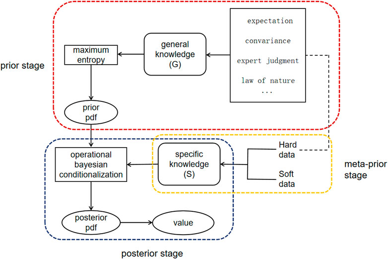
Figure 1. BME flow chart. BME mainly includes three stages: prior stage, meta-prior stage, and posterior stage. In the prior stage, maximum entropy is used to find the maximum amount of G information, while in the meta-prior stage, the data is expressed as specific knowledge S. In the posterior stage, $f_G$ and S need to be combined.

2.2.1.2 Hard and soft data

With the development of science and technology, data collection has become more diverse, faster, and more accurate and the scale range has expanded. In the BME method, data can be divided into two types according to the level of accuracy. One type is hard data, for which errors can be ignored or the accuracy is relatively high. These data are often measured by instruments or recorded at stations and include rainfall, pollutants, air pressure, and humidity recorded at meteorological stations, and ground motion parameters recorded at seismic stations, etc. The other type is soft data, for which errors are large or accuracy is relatively low; soft data are often obtained by empirical formulas, conclusions based on empirical intuition, or measurements with poor precision. The reason for describing the accuracy of data in this way is that, although the difference between hard and soft data is often quite clear, in some cases, it is a relative concept without a clear dividing line. This is similar to the nonexistence of observation instruments that can measure the true value without any error. The method of dividing data into hard and soft, as described, differs somewhat from the classification by Luo and Pei (2009) of data with definite true values (hard data) and data in “set” form (soft data). Hard data may objectively contain some errors, which are unavoidable, and to a certain extent, such results represent the true values, which fluctuates with conditions in real-word scenarios. In the data used in this paper, the results obtained from GMPE are less accurate than those obtained from seismic stations, so the GMPE results are soft data and the seismic network results are hard data. The forms of soft data often include interval data, probability data, and functional data, which are expressed by the following formulas. The distribution of soft data is shown in Figure 2.

(1) functional data, where l and u represent the lower and upper bounds of the interval, respectively

${\mathrm{\chi }}_{soft}={\left[x_{m_h}···x_m\right]}^T;{\chi }_i\in I_i=\left[l_i,u_i\right],i=m_{h+1}...m(\mathrm{2-3})$

(2) interval data, where ${\mathrm{F}}_{\mathrm{i}}\left({\mathrm{\zeta }}_{\mathrm{i}}\right)$ is the cumulative distribution function

${\mathrm{\chi }}_{soft}={\left[x_{m_h}···x_m\right]}^T;P\left({\chi }_i<{\zeta }_i\right)=F_i\left({\zeta }_i\right),i=m_{h+1}...m(\mathrm{2-4})$

(3) probability data, where $\mathrm{P}\left({\mathrm{\chi }}_{\mathrm{i}}\in {\mathrm{I}}_{\mathrm{i}}\right)={\mathrm{p}}_{\mathrm{i}}$ is a known function

${\mathrm{\chi }}_{soft}={\left[x_{m_h}···x_m\right]}^T;P\left({\chi }_i\in I_i\right)=p_i,i=m_{h+1}...m(\mathrm{2-5})$

Figure 2

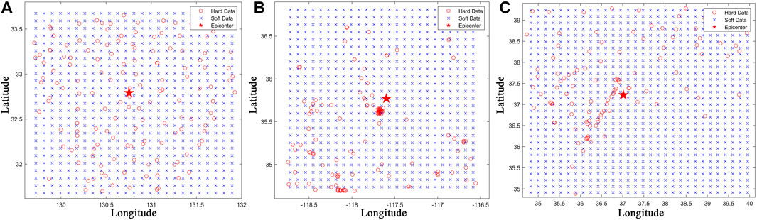
Figure 2. Distribution locations of the hard and soft data for the Japan earthquake, US earthquake, and Turkey earthquake. (A) is the Japan earthquake, (B) is the US earthquake, and (C) is the Turkey earthquake.The red pentagram is the epicenter, the red circles denote the distribution of hard data, and the blue x symbols denote the distribution of soft data.

2.2.2 GMPE

This paper uses the GMPE as soft data. Si et al. used multiple earthquake datasets in Japan, including crustal, intraplate and interplate earthquakes, and selected many close-range strong ground motion records for numerical simulation. The datasets have three characteristics, including strong ground motion records near the epicenter, an earthquake magnitude range of 5.8–8.3, and many types of seismogenic faults, and the focal depth distribution range is wide (6–120 km). After considering the epicenter characteristics, propagation characteristics, and site effects, we propose distance attenuation formulas for peak ground acceleration (PGA) and PGV based on the shortest distance from the fault, which are applicable to the epicenter region, i.e., the attenuation model for ground motion parameters (hereinafter referred to as the Si model). This model has achieved good application results for the 2008 Wenchuan earthquake (Si et al., 2010; Chen et al., 2022c).

$logA=b-\log \left(X+c\right)-kX(\mathrm{2-6})$

$c=c_1{10}^{{c_2}^{M_w}}(\mathrm{2-7})$

$b=a{M}_w+hD+\sum d_i{S}_i+e+\epsilon (\mathrm{2-8})$

$\log \left(\text{AMP}\right)=1.83-0.66\lg \left({\mathrm{v}}_{\mathrm{S}30}\right)(\mathrm{2-9})$

$PGV\_V_{S30}=AMP·PGV(\mathrm{2-10})$

where A is the PGA or PGV, $m/s^2$ and $m/s$; $PGV\_V_{S30}$ is the PGV after considering the site amplification effect, $m/s$; $M_w$ is the moment magnitude of the earthquake; c1 and c2 are regression coefficients, and the c1 in PGA is 0.0055, in PGV is 0.0028, and c2 is both 0.5; D is the focal depth, km; X is the shortest fault projection distance, km; AMP is the factor for the amplification effect; Vs30 is the equivalent shear wave velocity within the depth range of 30 m; and the k value is set to 0.003 for PGA and 0.002 for PGV, as shown in Table 2.

Table 2

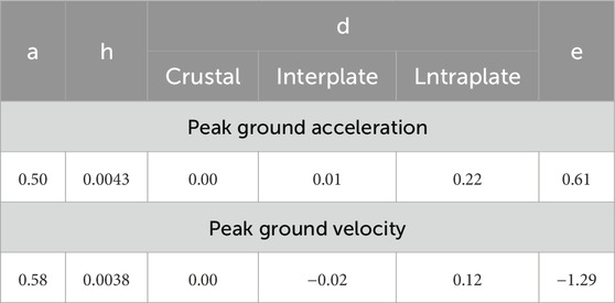
Table 2. Model parameters.

2.2.3 Wells empirical relationships

In Eqs 2–6, the earthquake fault distance is used to calculate the ground motion parameters, and the actual surface rupture zone is obtained in the actual investigation after an earthquake. The investigation period is approximately several weeks to several months, so the actual earthquake rupture zones cannot be obtained shortly after an earthquake. To consider the time cost after an earthquake, the Wells surface rupture empirical formula is used to obtain the surface rupture length instead of the actual length, and the final GMPE result can be obtained in seconds after an earthquake. In 1994, Wells used the epicenter parameters of historical earthquakes worldwide to establish the empirical relationships between moment magnitude and surface rupture length, subsurface rupture length and rupture area, and empirical relationships for strike slip faulting (SS), reverse faulting R), and normal faulting N) were established (Wells and Coppersmith, 1994). In this study, the rupture zones obtained based on the Wells formula are sampled uniformly at a distance of 1 km to calculate the shortest fault projection distance for each site. The fracture formulas are as follows:

$\text{SS}:\mathrm{M}=5.16+1.12\text{lg}\left(\mathrm{L}\right)(\mathrm{2-11})$

$\mathrm{R}:\mathrm{M}=5+1.22\text{lg}\left(\mathrm{L}\right)(\mathrm{2-12})$

$\mathrm{N}:\mathrm{M}=4.86+1.32\text{lg}\left(\mathrm{L}\right)(\mathrm{2-13})$

where L is the length of rupture, M is the moment magnitude.

3 Results

3.1 BME analysis results

Figure 3 represents the results of the covariance model, with the horizontal axis indicating the lag distance and the vertical axis displaying covariance values. This graph is generated through station data computations and involves two main steps: 1. Calculate the lag distance, which is the geographical distance between two data points, and 2. Calculate the covariance value for each lag distance. Covariance refers to the average of the squared differences between data points at the same lag distance. The following formula expresses this process:

$Cov\left(z\left(x\right),z\left(x+h\right)\right)=E\left\{z\left(x\right)-E\left[z\left(x\right)\right]\right\}\left\{z\left(x+h\right)-E\left[z\left(x+h\right)\right]\right\}(\mathrm{3-1})$

where h is the distance between one random variable to another random variable. $z\left(x\right)$ and $z\left(x+h\right)$ and are the values of random variables at spatial locations $x$ and $x+h$, respectively. $E\left[z\left(x\right)\right]$ and $E\left[z\left(x+h\right)\right]$ are the means at spatial locations $x$ and $x+h$, respectively.

Figure 3

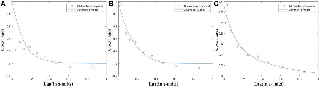
Figure 3. Fitting results for three seismic covariance models. The red circles are the all-directions empirical results, and the blue line is the covariance model fitting line. (A) is the Japan earthquake, (B) is the US earthquake, and (C) is the Turkey earthquake.

Curve fitting is employed to derive a mathematical equation, which is used to describe the relationship between covariance and lag distance, as described in the article. This curve can be utilized for interpolation and prediction purposes. A prior PDF is established through a covariance model of hard data. In the most affected areas of earthquakes, the seismic intensity is elliptically distributed, and for moderate and strong earthquakes. Several countries such as Japan, the US, and China are mainly affected by moderate earthquakes. According to Wells and Coppersmith (1994), the calculated rupture length for moderate earthquakes (magnitude 6.5-7.5) is generally about 100 km. So, the length of the hardest-hit area along the long axis is approximately 100 km. Therefore, correlations within a spatial range of approximately 100 km are selected to establish the empirical covariance model, and the results are shown in Figure 3. The Japan and US earthquakes are both Mw7 earthquakes. The curves in Figures 3A, B are roughly the same. The station values of the Japan earthquake within 30 km of the epicenter are relatively discrete, but they do not affect the overall spatial correlation. Due to the differences in geological structures and site conditions between Japan and the US, the attenuation details of the covariance models between the two are not exactly the same. As shown in Figure 3C, the magnitude of the Turkey M7.8 earthquake in 2023 is relatively large; earthquakes with large variable ranges attenuate faster for a certain distance, and the fitting of the covariance model is thus better. However, spatially correlated details for factors associated with large earthquakes are often overlooked. Figure 3 illustrates the strong spatial correlations among ground motion parameters, and the use of appropriate spatial interpolation methods can compensate for the shortcomings caused by an insufficient seismic station layout.

According to the BME conditional probability formula, the prior PDF is modified considering both hard and soft data, and the posterior PDF is obtained. According to the research, the appropriate BME prediction results are obtained with ${\mathrm{f}}_{\mathrm{K}}\left({\mathrm{\chi }}_{\mathrm{k}}\right)$; i.e., the prediction with the largest probability can be obtained from the prediction mode. Additionally, the prediction with the smallest mean square error can be obtained from the prediction mean, and the formula is the indefinite integral of the product of a random variable ${\mathrm{\chi }}_{\mathrm{k}}$ with the posterior PDF ${\mathrm{f}}_{\mathrm{K}}\left({\mathrm{\chi }}_{\mathrm{k}}\right)$, the prediction with the smallest mean absolute error (MAE) can be obtained from the prediction median. In this paper, the minimum mean square error is selected as the BME prediction result. The results are shown in Figure 4. Figures 4A, C, E show the prediction means of the three earthquakes, and b), d), and f) are three-dimensional (3D) maps of the standard deviation (SD) of the prediction results. The unit of SD here is consistent with the unit of PGV, both in m/s. The predicted SD of the three earthquakes within the epicenter region is high, and the SD of the low-intensity zones away from the epicenter is extremely low and tends to be close to zero. For the 7.8-magnitude earthquake in Turkey, in the hard-hit area (longitude 36°–38°E and latitude 36°–38°N), the SD of predictions reaches 0.76, which seriously exceeds the mean SD. The SD of the Japan and US earthquakes is lower, and the prediction effect is better, particularly compared to that of the Turkey earthquake, Notably, for the 7-magnitude US earthquake, SD < 0.3. The magnitude and affected area of the Turkey earthquake are larger than those of the Japan and US earthquakes; therefore, with the same number of stations, the BME prediction results for the Turkey earthquake are not as good as those for the Japan and US earthquakes.

Figure 4

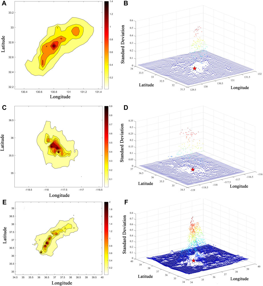
Figure 4. BME analysis results and 3D maps of BME SD. The contour line interval in a, c, and e is 0.1. (A) is the BME result for the Japan earthquake; (C) is the BME result for the US earthquake; (E) is the BME result for the Turkey earthquake; (B) is the BME SD result for the Japan earthquake, with red representing higher values and blue representing lower values; (D) is the BME SD result for the US earthquake; (F) is the BME SD result for the Turkey earthquake.

3.2 Intensity analysis results

Contour lines are generated at an interval of 0.1 (Figures 4A–C); however, it is impossible to see the pros and cons of the prediction results for actual earthquakes based on contour lines alone. ShakeMap is used internationally as an important seismic service platform that can support different seismic assessments for earthquakes in various regions and at various levels. One of the main assessment methods involves reclassifying ground motion parameters according to the MMI and standardizing the extent of the hardest-hit areas of earthquakes, with MMI values ≥ degree VIII defined as moderately or severely damaged. Thus, focus is placed on events with values ≥ degree VIII. The prediction results in Figures 4A–C are converted into MMI results for unified evaluation and compared with the ShakeMap results, as shown in Figure 6.

To test whether ShakeMap results can be used to verify the BME analysis results, the root mean square error (RMSE) is selected as an indicator, and the BME and ShakeMap results for the Japan earthquake are evaluated. According to the calculation results, for the Japan earthquake, the RMSEs of the BME prediction result and ShakeMap prediction result are 0.07 and 0.06, respectively, which verifies that the accuracy of ShakeMap is slightly higher than that of the BME method. In addition, to better illustrate the similarities between the BME and ShakeMap method, a residual analysis process was implemented (Figure 5). For the Japan earthquake and the US earthquake, there are no significant differences between the results obtained with the BME and ShakeMap method. In the case of the earthquake in Turkey, when compared to the BME results, the ShakeMap predictions show an overall trend of residuals approaching zero. However, within 100 km of the epicenter, there is still no noticeable difference between the two sets of results, and the BME prediction accuracy remains within 0.6. The high degree of similarity between the results from the BME and ShakeMap method is evident from the residual analysis, underscoring the utility of ShakeMap for validating the prediction results in this study.

Figure 5

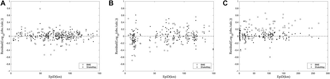
Figure 5. Residual analysis. The abscissa is the epicenter distance, and the ordinate is the logarithmic ratio of the measured data to the predicted data. Comparison of the results of the ShakeMap and BME method for the (A) Japan earthquake, (B) US earthquake and (C) Turkey earthquake.

The BME prediction results for the Japan, US and Turkey earthquakes are converted into MMI values and compared with the ShakeMap results, as shown in Figures 6A–C. Figures 6D–F shows the soft data results corresponding to the three earthquakes. In Figures 6A, D, for the Japan earthquake, the predictions based on the BME results and soft data results for the areas < degree VIII are consistent. Based on both the BME results and soft data results, the hardest-hit areas are overpredicted in comparison to those based on the ShakeMap results. For the soft data results, the intensity to the southwest of the epicenter is high, with many degree-IX areas, which differ significantly from the ShakeMap results; additionally, the intensity to the northeast of the epicenter is in comparatively better agreement with the ShakeMap results. For the BME results, there is only a degree-IX area at the epicenter, and there is an extended zone of degree-VIII areas to the southwest; however, compared to the soft data results, the BME results provide a more reliable direction and scope for postearthquake emergency response. According to Figures 6B, E, the US earthquake is similar to the Japan earthquake, but the BME results are not ideal due to the deviation between the rupture directions predicted based on the US earthquake soft data and the ShakeMap results. However, the degree-VIII and degree-IX areas mispredicted in the soft data results are largely corrected with the BME method. The results for the Turkey earthquake show that the BME method corrects some of the degree-IX areas, but the effect on the overall results is small. The BME correction strength for large earthquakes is not as significant as that for small earthquakes, which may be related to the large area of large earthquakes and the lack of updating of soft data results due to a limited number of stations, indicating that the method proposed in this paper can be reliably used to determine the extent of the hardest-hit areas of moderate to strong earthquakes. Therefore, the soft data have a large effect on the final posterior PDF $f_K\left({\chi }_k\right)$.

Figure 6

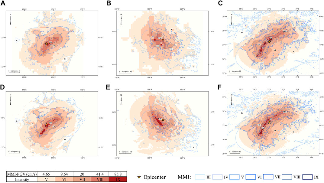
Figure 6. Comparison of the BME analysis results and the soft data results obtained with ShakeMap, the blue line is the MMI result obtained with ShakeMap. The converted MMI results from the BME method for the (A) Japan earthquake, (B) US earthquake and (C) Turkey earthquake are shown; The converted MMI result from soft data for the (D) Japan earthquake, (E) US earthquake and (F) Turkey earthquake.

4 Discussion

4.1 Reliability analysis

Zhao et al. (2023) analyzed the profiles of the Maduo earthquake and the Maerkang earthquake in China, and the analysis method used clearly and directly verified the reliability of the two sets of seismic intensity assessment results. In this paper, a profile line is drawn along the long axis of the ShakeMap isoseismal lines for the Japan, US and Turkey earthquakes, inverse distance weighted (IDW) and kriging interpolations are performed using hard data, and the interpolation results and BME results are analyzed. Figures 7A–C shows that, although the IDW and kriging results for the Japan earthquake are consistent with the ShakeMap results at the epicenter, they are one degree lower than the ShakeMap results in other areas. In practice, this difference can be ignored because the area is close to the epicenter. In addition, the BME results in some degree-VIII areas and the half of the remaining areas are inconsistent with the ShakeMap results, generally indicating that the evaluation results are satisfactory. For the US earthquake, the highest intensity estimated with the three prediction methods is consistent with that based on the ShakeMap results, but there are inconsistencies in other directions, which are caused by the inconsistency between the assessment direction of and the rupture direction, and the results of the three methods are less than satisfactory, as shown in Figures 7D–F. The profiles of the 2023 Turkey earthquake are shown in Figures 7G–I. The highest intensity results of the three methods for the IDW, kriging, and BME methods are all consistent. The BME results are similar to the ShakeMap results, and IDW may yield intensity anomalies in low-intensity areas; therefore, the IDW results cannot be used. The profile results of the three earthquakes directly or indirectly reflect the reliability of the BME approach in seismic intensity assessment.

Figure 7

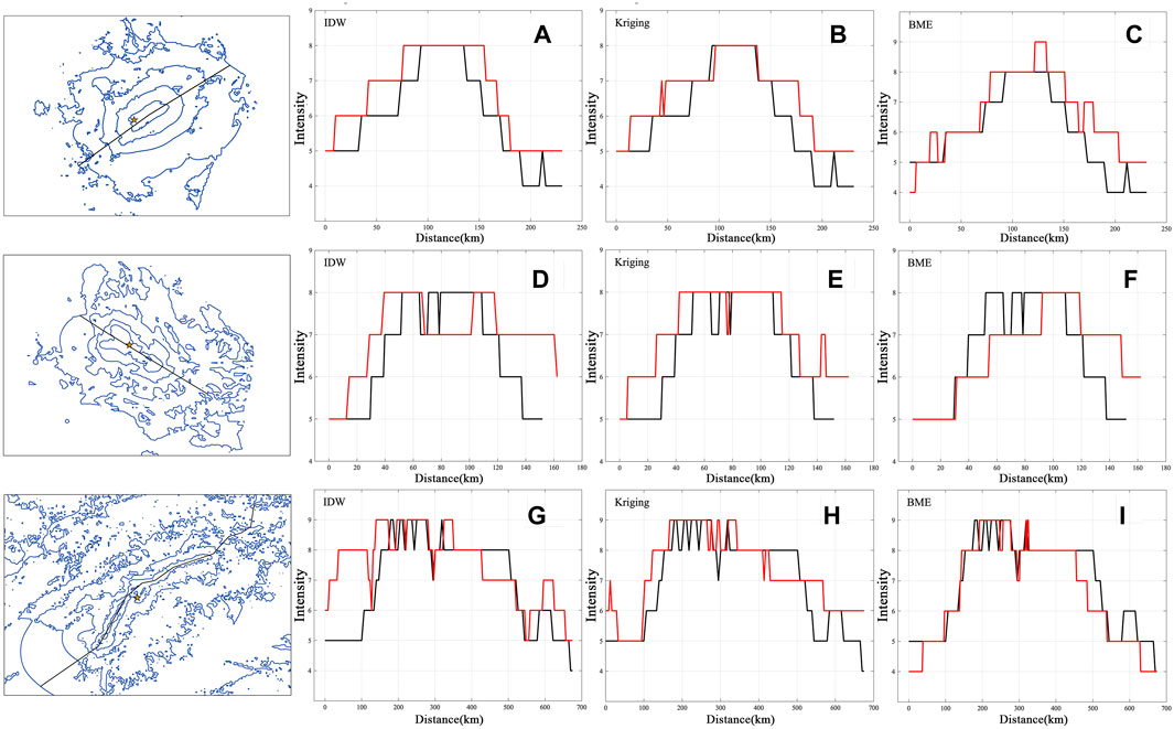
Figure 7. Seismic intensity profile. The solid black line represents the location of the profile, and the red line is the profile produced by the model. (A), (B), and (C) are the profiles obtained with the IDW, kriging, and BME methods for the Japan earthquake; (D), (E), and (F) are the profiles obtained with the IDW, kriging, and BME methods for the US earthquake; and(G), (H), and (I) are the profiles obtained with the IDW, kriging, and BME methods for the Turkey earthquake.

Compared to the MAE, the RMSE is calculated with a differentiable function, which makes it easy to perform mathematical operations. Therefore, in many models, although RMSE is more difficult to interpret than MAE, it is used as the default metric for establishing the loss function, as shown in Figure 8. Residual error generally refers to the difference between the predicted and observed values, and is also one of the important indicators used to evaluate the quality of a prediction result, as shown in Figure 9. The BME analysis in this paper is mainly Bayesian estimation. The predicted value is obtained from a PDF based on a combination of soft data and hard data, and hard data are not directly used to obtain the prediction result. Hard data are often limited and difficult to obtain. To consider the accuracy of the prediction results and the comprehensiveness of the evaluation, in this paper, data from no stations are retained for testing; thus, hard data are only used for residual analysis and RMSE analysis of stations.

Figure 8

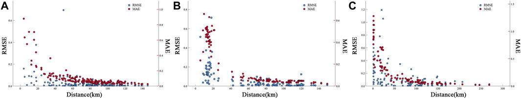
Figure 8. RMSE and MAE analysis diagram, where red is MAE and blue is RMSE. The RMSE and MAE results for the (A) Japan earthquake, (B) US earthquake, and (C) Turkey earthquake.

Figure 9

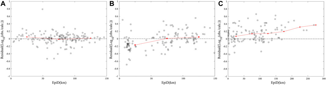
Figure 9. Residual analysis for PGV. The abscissa is the epicenter distance, and the ordinate is the logarithmic ratio of the measured data to the predicted data. The residual results for the (A) Japan earthquake, (B) US earthquake and (C) Turkey earthquake.

According to the RMSE results, the prediction effects for the Turkey earthquake (Figure 8C) and US earthquake (Figure 8B) are not as good as those for the Japanese earthquake (Figure 8A). The highest RMSE for the Turkey earthquake reaches approximately 1.1, and that for the US earthquake exceeds 0.7; however, the RMSE for the Japan earthquake is higher than 0.2 at only two stations, indicating that the prediction effect is comparatively better. The RMSE of the three earthquakes is overestimated around the epicenter, and the RMSE in the far-field range does not exceed 0.2, which shows that the evaluation of ground motion parameters near major faults is difficult. When stations are located near the epicenter, limited station data are obtained, with many outliers, leading to the above phenomenon. Based on the prediction results of the three earthquakes, the BME method still yields good predictive power for moderate and strong earthquakes. As shown in Figure 9, the residuals of the Japan earthquake in Figure 9A are between −0.6 and 0.4, those of the US earthquake in Figure 9B are between −0.6 and 0.6, and those of the Turkey earthquake in Figure 9C are between −0.4 and 0.8, indicating that the BME-based values for major earthquakes are mainly underpredicted. Due to the prediction direction problem encountered for the US earthquake, the phenomenon of overprediction at the epicenter occurs. The prediction mean for the Japan earthquake at 50 km is close to 0, indicating that the calculated ground motion is close to the observed value, which verifies the stability of the method proposed in this paper.

4.2 Applicable conditions

The BME spatial interpolation method based on the attenuation formula combined with the strong ground motion data presented in this paper requires the observation results at seismic stations to be obtained during and immediately after an earthquake. Additionally, a sufficient number of stations must be available; otherwise, the posterior PDF cannot be obtained through updating the prior PDF (or the results are dominated by soft data-based results). Notably, due to various uncontrollable factors, the quality of station monitoring data varies, so it is particularly important to consider how to screen high-quality stations and determine whether the station data are seismic intensity anomalies in the context of providing a rapid postearthquake emergency response. Peak Ground Acceleration (PGA) is one of the important indicators for measuring earthquake intensity. It reflects the maximum ground acceleration during an earthquake, and higher PGA values are usually associated with more severe seismic intensity. Especially for building and infrastructure engineering, PGA is one of the key factors in evaluating whether the structural design is strong enough to withstand earthquake forces. Experts use PGA values to determine the design parameters of structures such as buildings and bridges to ensure their safety during earthquakes (Tselentis and Danciu, 2008; Murphy and O’brien 1977; Campbell, 1997). However, some studies have shown that the correlation between PGV and seismic damage statistics is closer than that of PGA (Wu et al., 2003). Therefore, in this section, we will discuss the applicability of PGA in BME. As shown in Figure 10 below, the PGA result of the US earthquake in Figure 10B is obviously inferior to that of the Japanese earthquake and the Turkey earthquake. By comparing the PGV residual results in Figure 9, we can find that the PGV results of both the Japanese earthquake and the American earthquake are better, and the PGV results of the Turkey earthquake are better, which can certainly indicate that the PGA results are more accurate in the case of catastrophic earthquake. The research results for the three earthquakes (Japan, US and Turkey earthquakes) clearly show that when the station data are similar, the BME method is not ideal for predicting the ground motion from the earthquakes with larger areas but performs better for moderate and strong earthquakes. Therefore, in a large-earthquake cases, the prediction results of the attenuation formula are sufficient to make a basic assessment of the large earthquake. Compared with that for the US earthquake, the prediction effect for the Japan earthquake was better. We speculate that the attenuation formula in this paper was established by Si based on the Japan dataset, so the results are more suitable for earthquakes in Japan; therefore, if different attenuation formulas are used for different regions, the accuracy of BME predictions may be improved. In the US earthquake, the direction of the earthquake rupture is inconsistent with the predicted direction, resulting in low prediction accuracy, which is caused by the inconsistency in the direction of the nearest fault selected around the epicenter. Due to the presence of many active faults around the earthquake, which makes it difficult to select the correct faults in the blind period after the earthquake, other methods, such as the back-projected energy point approach or an aftershock data method, can be used instead of selecting the nearest fault to improve the quality of the soft data; this will be the focus of future works. Although the BME approach is a spatiotemporal analysis method, the time factor is not included in this paper, even though a seismic wave is a time–history curve; therefore, determining how to combine spatial and temporal factors to obtain more accurate results is a topic worthy of further study.

Figure 10

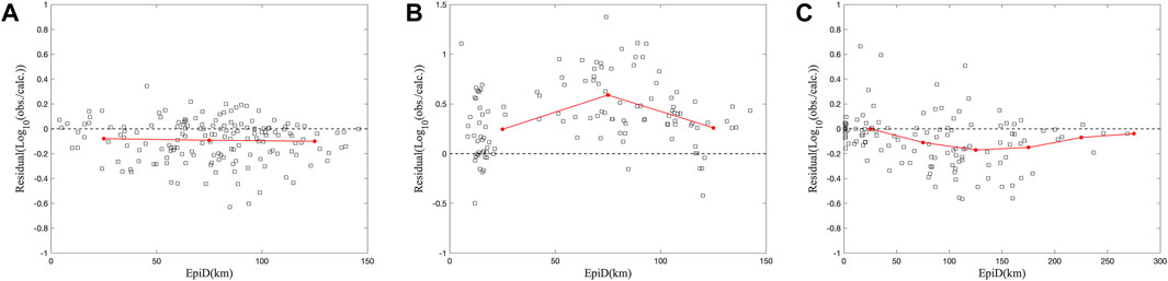
Figure 10. Residual analysis for PGA. The abscissa is the epicenter distance, and the ordinate is the logarithmic ratio of the measured data to the predicted data. The residual results for the (A) Japan earthquake, (B) US earthquake and (C) Turkey earthquake.

5 Conclusion

In this paper, for the first time, we propose a BME spatial interpolation method that combines soft data and hard data for seismic intensity assessment. In the proposed method the prior PDF is obtained based on kriging interpolation analysis of the strong ground motion data after an earthquake, soft data obtained based on an attenuation formula are considered, soft and hard data with certain ranges near a given prediction point are used to obtain the posterior PDF, and the desired maximum or mean is calculated by conversion. Finally, seismic intensity maps are quickly plotted based on the calculation results of the ground motion data from the posterior PDF; in this approach, hard data are used twice, and the weights of station data are higher than those for the results of the attenuation formula. The main contributions of the paper are as follows.

(1) The BME approach is a highly popular interpolation method. Although maximizing the amount of hard data used can improve the accuracy of the method, when only soft data or limited station data are available, the method can still yield reasonable results. Thus, the BME method can be used in interpolation analyses in many study areas.

(2) The interpolation of the ground motion data for the three earthquakes in this paper shows that the proposed method is effective for the prediction of moderate and strong earthquakes. The station density is generally homogeneous in space. Although more station data are obtained for major earthquakes than for smaller earthquakes, most recorded values are in the same intensity zones, with little effect on the interpolation results. For earthquakes with small moment magnitudes (Mw6-7), the predictions of the proposed method are better than those of other methods. The proposed method compensates for the phenomenon that the traditional attenuation formula is insufficient for predicting earthquakes with small moment magnitudes. Additionally, the BME method mitigates the large deviation between predicted and actual damage levels when the moment magnitudes are small. Combined with SEKS GUI software, the proposed method has a simple operation process and can quickly produce a seismic intensity assessment map, which is helpful for providing earthquake disaster information services.

(3) The BME method proposed in this paper is a combination of an attenuation formula and station data, which enriches the existing seismic intensity assessment methods to a certain extent. At the same time, the problems arising from the application of the method could in turn provide a new basis for the selection of the actual rupture direction and optimization of soft data methods for earthquakes.

(4) Considering the time factor of rapid assessment of earthquake intensity after an earthquake, the method (BME) of combining a simplified GMPE with stations can obtain earthquake emergency assessment results faster than ShakeMap with MNV and NGA West 2 GMPE. Therefore, BME can provide evaluation results of the “black box period” after an earthquake, enriching the means and methods of rapid post-earthquake evaluation.

Data availability statement

The raw data supporting the conclusion of this article will be made available by the authors, without undue reservation.

Author contributions

DK: Investigation, Methodology, Software, Visualization, Writing–original draft, Writing–review and editing. WC: Funding acquisition, Supervision, Validation, Writing–review and editing. YJ: Formal Analysis, Writing–review and editing.

Funding

The author(s) declare that financial support was received for the research, authorship, and/or publication of this article. This research was funded by the Fundamental Research Funds in the Institute of Earth-quake Forecasting, China Earthquake Administration (grant number 2023IESLZ04), the National Key Research and Development Program of China (grant number 2017YFB0504104).

Conflict of interest

The authors declare that the research was conducted in the absence of any commercial or financial relationships that could be construed as a potential conflict of interest.

Publisher’s note

All claims expressed in this article are solely those of the authors and do not necessarily represent those of their affiliated organizations, or those of the publisher, the editors and the reviewers. Any product that may be evaluated in this article, or claim that may be made by its manufacturer, is not guaranteed or endorsed by the publisher.

References

An, Y., Wang, D., Ma, Q., Xu, Y., Li, Y., Zhang, Y., et al. (2023). Preliminary report of the September 5, 2022 MS 6.8 Luding earthquake, Sichuan, China. Earthq. Research. Adv. 3 (1), 100184.

CrossRef Full Text | Google Scholar

Atkinson, G. M., and Sonley, E. (2000). Empirical relationships between modified Mercalli intensity and response spectra. Bull. Seismol. Soc. Am. 90 (2), 537–544. doi:10.1785/0119990118

CrossRef Full Text | Google Scholar

Atkinson, G. M., and Wald, D. J. (2007). “Did You Feel It?” intensity data: a surprisingly good measure of earthquake ground motion. Seismol. Res. Lett. 78, 362–368. doi:10.1785/gssrl.78.3.362

CrossRef Full Text | Google Scholar

Boore, D. M., Stewart, J. P., Seyhan, E., and Atkinson, G. M. (2014). NGA-West2 equations for predicting PGA, PGV, and 5% damped PSA for shallow crustal earthquakes. Earthq. Spectra 30 (3), 1057–1085. doi:10.1193/070113eqs184m

CrossRef Full Text | Google Scholar

Campbell, K. W. (1997). Empirical near-source attenuation relationships for horizontal and vertical components of peak ground acceleration, peak ground velocity, and pseudo-absolute acceleration response spectra. Seismol. Res. Lett. 68 (1), 154–179. doi:10.1785/gssrl.68.1.154

CrossRef Full Text | Google Scholar

Campbell, K. W., and Bozorgnia, Y. (2014). NGA-West2 ground motion model for the average horizontal components of PGA, PGV, and 5% damped linear acceleration response spectra. Earthq. Spectra 30 (3), 1087–1115. doi:10.1193/062913eqs175m

CrossRef Full Text | Google Scholar

Chen, J., Tang, H., Chen, W., and Yang, N. (2022a). A prediction method of ground motion for regions without available observation data (LGB-FS) and its application to both yangbi and Maduo earthquakes in 2021. J. Earth Sci. 33 (4), 869–884. doi:10.1007/s12583-021-1560-6

CrossRef Full Text | Google Scholar

Chen, W., Wang, D., Si, H., and Zhang, C. (2022b). Rapid estimation of seismic intensities using A new algorithm that incorporates array technologies and ground-motion prediction equations (gmpes). Bull. Seismol. Soc. Am. 112 (3), 1647–1661. doi:10.1785/0120210207

CrossRef Full Text | Google Scholar

Chen, W. K., Wang, D., Zhang, C., Yao, Q., and Si, H. (2022c). Estimating seismic intensity maps of the 2021 Mw 7.3 madoi, Qinghai and Mw 6.1 yangbi, yunnan, China earthquakes. J. Earth Sci. 33, 839–846. doi:10.1007/S12583-021-1586-9

CrossRef Full Text | Google Scholar

Chen, W., Rao, G., Kang, D., et al. (2023). Early report of the source characteristics, ground motions, and casualty estimates of the 2023 Mw 7.8 and 7.5 Turkey earthquakes. J. Earth Sci. 34 (2), 297–303.

CrossRef Full Text | Google Scholar

Christakos, G. (1990). A Bayesian/maximum-entropy view to the spatial estimation problem. Math. Geol. 22 (7), 763–777. doi:10.1007/bf00890661

CrossRef Full Text | Google Scholar

Christakos, G. (2000). Modern spatiotemporal geostatistics. New York, NY: Oxford Univ Press. New edition: Dover Publ Inc., Mineola, NY.

Google Scholar

Christakos, G., Kolovos, A., Serre, M. L., and Vukovich, F. (2004). Total ozone mapping by integrating databases from remote sensing instruments and empirical models. Ieee T Geosci. Remote 42 (5), 991–1008. doi:10.1109/tgrs.2003.822751

CrossRef Full Text | Google Scholar

Christakos, G., and Li, X. (1998). Bayesian maximum entropy analysis and mapping: a farewell to kriging estimators? Math. Geol. 30 (4), 435–462. doi:10.1023/a:1021748324917

CrossRef Full Text | Google Scholar

Coulliette, A. D., Money, E. S., Serre, M. L., and Noble, R. T. (2009). Space/time analysis of fecal pollution and rainfall in an eastern North Carolina estuary. Environ. Sci. Technol. 43 (10), 3728–3735. doi:10.1021/es803183f

PubMed Abstract | CrossRef Full Text | Google Scholar

Douaik, A., Van Meirvenne, M., and Toth, T. (2005). Soil salinity mapping using spatio-temporal kriging and Bayesian maximum entropy with interval soft data. Geoderma 128 (3-4), 234–248. doi:10.1016/j.geoderma.2005.04.006

CrossRef Full Text | Google Scholar

Gehl, P., Douglas, J., and D'Ayala, D. (2017). Inferring earthquake groundmotion fields with Bayesian networks. Bull. Seismol. Soc. Am. 107, 2792–2808. doi:10.1785/0120170073

CrossRef Full Text | Google Scholar

Guo, Y., Li, H., Liang, P., Xiong, R., Hu, C., and Xu, Y. (2024). Preliminary report of coseismic surface rupture (part) of Türkiye's MW7. 8 earthquake by remote sensing interpretation. Earthq.Research Adv. 4 (1), 100219.

CrossRef Full Text | Google Scholar

Jia, Y., Chen, W., Kang, D., et al. (2023). Rapid determination of source parameters of the M6.2 Jishishan earthquake in Gansu Province and its application in emergency response[J]. Earthq. Research Adv. doi:10.1016/j.eqrea.2024.100310

CrossRef Full Text | Google Scholar

Kang, D., Chen, W., Zhao, H., et al. (2023). Rapid assessment of the September 5, 2022 MS 6.8 Luding earthquake in Sichuan, China[J]. Earthq. Research. Adv. 3 (2), 100214.

CrossRef Full Text | Google Scholar

Kinoshita, S. (1998). Kyoshin net (K-net). Seismol. Res. Lett. 69 (4), 309–332. doi:10.1785/gssrl.69.4.309

CrossRef Full Text | Google Scholar

Krinitzsky, E. L., and Chang, F. K. (1988). Intensity-related earthquake ground motions. Bull. Assoc. Eng. Geol. 25 (4), 425–435. doi:10.2113/gseegeosci.xxv.4.425

CrossRef Full Text | Google Scholar

Luo, M., and Pei, T. (2009). Review on soft spatial data and its spatial interpolation methods. Prog. Geogr. 28 (05), 663–672. doi:10.11820/dlkxjz.2009.05.003

CrossRef Full Text | Google Scholar

Money, E. S., Carter, G. P., and Serre, M. L. (2009). Modern space/time geostatistics using river distances: data integration of turbidity and E. coli measurements to assess fecal contamination along the Raritan River in New Jersey. Environ. Sci. Technol. 43 (10), 3736–3742. doi:10.1021/es803236j

PubMed Abstract | CrossRef Full Text | Google Scholar

Murphy, J. U., and O'brien, L. J. (1977). The correlation of peak ground acceleration amplitude with seismic intensity and other physical parameters. Bull. Seismol. Soc. Am. 67 (3), 877–915. doi:10.1785/bssa0670030877

CrossRef Full Text | Google Scholar

Peng, C., Jiang, P., Ma, Q., Wu, P., Su, J., Zheng, Y., et al. (2021). Performance evaluation of an earthquake early warning system in the 2019-2020 M 6.0 changning, sichuan, China, seismic sequence. Front. Earth Sci. 9, 699941. doi:10.3389/feart.2021.699941

CrossRef Full Text | Google Scholar

Peng, Y., and Wang, D. (2023). Multiple point source-based W-phase inversion and its application to the Sumatra MW9.1earthquake in 2004. China J. Earthq. Eng. 45 (01), 169–180.

Google Scholar

Si, H., Hao, K. X., Xu, Y., Senna, S., Fujiwara, H., Yamada, H., et al. (2010). “Attenuation characteristics f peak ground motions during the Mw7.9 wenchuan earthquake, China,” in 7th International Conference on Urbanearthquake Engineering (7CUEE) and. 5th International Conference on Earthquake Engineering (5ICEE).

Google Scholar

Si, H., and Midorikawa, S. (1999). New attenuation relationships for peak ground acceleration and velocity considering effects of fault type and site condition. J. Struct. Constr. 64, 63–70. doi:10.3130/aijs.64.63_2

CrossRef Full Text | Google Scholar

Smith, E. M., and Mooney, W. D. (2021). A seismic intensity survey of the 16 april 2016 Mw 7.8 pedernales, Ecuador, earthquake: a comparison with strong-motion data and teleseismic backprojection. Seismol. Res. Lett. 92, 2156–2171. doi:10.1785/0220200290

CrossRef Full Text | Google Scholar

Trifunac, M. D., and Brady, A. G. (1975). A study on the duration of strong earthquake ground motion. Bull. Seismol. Soc. Am. 65 (3), 581–626. doi:10.1785/BSSA0650030581

CrossRef Full Text | Google Scholar

Tselentis, G. A., and Danciu, L. (2008). Empirical relationships between modified Mercalli intensity and engineering ground-motion parameters in Greece. Bull. Seismol. Soc. Am. 98 (4), 1863–1875. doi:10.1785/0120070172

CrossRef Full Text | Google Scholar

Wang, X., Dou, A., Wang, L., Yuan, X., Ding, X., and Zhang, W. (2015). RS-based assessment of seismic intensity of the 2013 Lushan, Sichuan, China M s7.0 earthquake. ChineseJ.Geophys. in Chin. 58 (1), 163–171. doi:10.6O38/cjg2O15O114

CrossRef Full Text | Google Scholar

Wang, Y., Jiang, C., and Liu, F. (2017). Evaluation of monitoring capability of China seismic network and scoring of station detection capability (2008-2015). Chin. J. Geophys. 60 (07), 2767–2778. doi:10.6038/cjg20170722

CrossRef Full Text | Google Scholar

Wells, D. L., and Coppersmith, K. J. (1994). New empirical relationships among magnitude, rupture length, rupture width, rupture area, and surface displacement. Bull. Seismol. Soc. Am. 84 (4), 974–1002. doi:10.1785/bssa0840040974

CrossRef Full Text | Google Scholar

Wibrin, M. A., Bogaert, P., and Fasbender, D. (2006). Combining categorical and continuous spatial information within the Bayesian maximum entropy paradigm. Stoch. Env. Res. Risk A 20 (6), 423–433. doi:10.1007/s00477-006-0035-8

CrossRef Full Text | Google Scholar

Worden, C. B., Gerstenberger, M. C., Rhoades, D. A., and Wald, D. J. (2012). Probabilistic relationships between ground-motion parameters and modified Mercalli intensity in California. Seism. Soc. Am. 102 (1), 204–221. doi:10.1785/0120110156

CrossRef Full Text | Google Scholar

Worden, C. B., Wald, D. J., Allen, T. I., Lin, K., Garcia, D., and Cua, G. (2010). A revised ground-motion and intensity interpolation scheme for ShakeMap. Bull. Seismol. Soc. Am. 100 (6), 3083–3096. doi:10.1785/0120100101

CrossRef Full Text | Google Scholar

Wu, Y. M., Teng, T. L., Shin, T. C., et al. (2003). Relationship between peak ground acceleration, peak ground velocity, and intensity in taiwan. Bull. Of Seismol. Soc. Of Am. 93 (1), 386–396. doi:10.1785/0120020097

CrossRef Full Text | Google Scholar

Xiao, L., Zheng, R., and Zou, R. (2022). Coseismic slip distribution of the 2021 Mw7.4 Maduo, Qinghai Earthquake Estimated from InSAR and GPS measurements. J. Earth Sci. 33 (4), 885–891.

CrossRef Full Text | Google Scholar

Yaghmaei-Sabegh, S., and Hassani, B. (2020). Investigation of the relation between Vs30 and site characteristics of Iran based on horizontal-to-vertical spectral ratios. Soil Dyn. Earthq. Eng. 128, 105899. doi:10.1016/j.soildyn.2019.105899

CrossRef Full Text | Google Scholar

Yu, H. L., Kolovos, A., Christakos, G., Chen, J. C., Warmerdam, S., and Dev, B. (2007). Interactive spatiotemporal modelling of health systems: the SEKS-GUI framework. Stoch Envir Res Risk Assess Special Volume Med. Geogr. as a Sci. Interdiscip. Knowl. Synthesis under Cond. Uncertain. 21 (5), 647–572. doi:10.1007/s00477-007-0172-8

CrossRef Full Text | Google Scholar

Yu, H. L., Wang, C. H., Liu, M. C., and Kuo, Y. M. (2011). Estimation of fine particulate matter in taipei using landuse regression and bayesian maximum entropy methods. Int. J. Environ. Res. Public Health 8 (12), 2153–2169. doi:10.3390/ijerph8062153

PubMed Abstract | CrossRef Full Text | Google Scholar

Zhao, H., He, S., Chen, W., Si, H., Yin, X., and Zhang, C. (2022). A rapid evaluation method of earthquake intensity based on the aftershock sequence: a case study of Menyuan M6. 9 earthquake in Qinghai Province. China Earthq. Eng. J. 44, 432–439. doi:10.20000/j.1000-0844.20220128002

CrossRef Full Text | Google Scholar

Zhao, H., Jia, Y., Chen, W., Kang, D., and Zhang, C. (2023). Rapid mapping of seismic intensity assessment using ground motion data calculated from early aftershocks selected by GIS spatial analysis. Geomatics, Nat. Hazards Risk 14 (1), 1–21. doi:10.1080/19475705.2022.2160663

CrossRef Full Text | Google Scholar

Zhou, Z., Sun, Y., and Zhu, R. (2024). Evaluation of post⁃earthquake buried personnel based on a new model of seismic intensity rapid assessment. Earth Sci. 49 (2), 437–450.

Google Scholar