Detecting differential item functioning in presence of multilevel data: do methods accounting for multilevel data structure make a DIFference?

Introduction

Educational and psychological assessment practices are, among other things, concerned with fairness and appropriate score interpretations. For example, data from international large-scale assessments (ILSAs), such as the Programme for International Student Assessment (PISA) or the Trends in International Mathematics and Science Study (TIMSS), are used to inform about student academic performance across dozens of participating countries and educational systems, which provides, in large part, the basis for educational reforms in those respective countries and educational systems. Further, constructs being measured on ILSAs ought not to be only cognitive in nature. PISA and TIMSS, in addition to measuring achievement in mathematics or science, also serve as a fruitful basis from which to derive measures of affective and motivational domains how students feel about school or learning (e.g., Ozel et al., 2013; Segeritz and Pant, 2013; Marsh et al., 2015).

Similarly, the Teaching and Learning International Survey (TALIS) measures and compares teachers’ attitudes, perceptions, and experiences related to education. Outside education, examples of studying psychological constructs across cultures abound, including social axioms (e.g., Bou Malham and Saucier, 2014), physical self-perception (e.g., Hagger et al., 2003), cognitive emotional regulation (e.g., Megreya et al., 2016), and identity processing styles during cultural transition (e.g., Szabo et al., 2016). Regardless of the context, scores that represent the underlying constructs of interest on surveys and assessments are often summarized in terms of total scores or model-based scale scores (Olson et al., 2008; Economic Co-operation and Development, 2010) which are then compared across the groups.

Across the aforementioned examples, and for many others found in social sciences, an important precursor to making meaningful comparisons across groups on scale scores involves the establishment of measurement invariance (MI). Namely, this criterion states that a construct ought to be understood and measured equivalently across groups of interest (Meredith, 1993). In practice, lacking MI has long been considered a threat to the validity of score interpretations and use based on such. Often times, researchers adopt the approach of multiple-groups confirmatory factor analysis (MG-CFA; Jöreskog, 1971) to examine if the structure of an assessment is the same across groups.

At the item level, MI indicates the absence of differential item functioning (DIF; Holland and Wainer, 2012). An item is said to be a DIF item when it exhibits different psychometric properties between individuals with similar proficiencies and from different groups (e.g., Croatian students vs. German students on ILSAs). DIF can be categorized as uniform when the relationship between the group membership and response to an item is constant for all levels of the matching proficiency (i.e., no interaction between group membership and ability), while non-uniform DIF is present when there exists such interaction. When two groups are considered, the group of interest in the analysis is referred to as the focal group, while the group to which focal group is compared to is known as the reference group.¹ The importance of identifying DIF items in educational measurement and assessment, as well as broadly defined social and psychological sciences, has been well established (e.g., Magis et al., 2010; Gao, 2019). Over the last few decades, a number of methods have been proposed to detect DIF items more accurately and thus aid in measurement or test development process, such as the score-based Mantel–Haenszel procedure (score-based MH; Mantel and Haenszel, 1959; Holland and Thayer, 1988; Narayanon and Swaminathan, 1996), and the model-based Lord’s Wald χ² test (model-based Lord, 1980). If an item is determined to be differentially functioning–meaning, it is flagged as a DIF item–test developers can choose whether to revise or remove it dependent on what sources of DIF are determined to be.

Magis et al. (2010) presented a useful framework for researchers to select and employ a DIF detection method in their analysis when data are scored dichotomously (e.g., 0 as incorrect/disagree; 1 as correct/agree). Specifically, the authors organized DIF detection methods along four main dimensions the methods are able to accommodate: (a) number of focal groups (two vs. > 2), (b) methodological approach in creating a matching variable (Item Response Theory-based vs. Classical Test Theory-based), (c) DIF type (uniform vs. non-uniform), and (d) item purification (considered). These four dimensions highlight important considerations/aspects a researcher ought to engage with when conducting DIF analysis with the ultimate aim to make appropriate and valid claims. Alongside the proposed framework, Magis and his colleagues developed an R package called difR (Magis et al., 2010) which included a collection of standard DIF detection methods for dichotomous items. As described below, in the current study, we utilized two DIF detection methods employed in difR—specifically, the single-level MH method (Mantel and Haenszel, 1959) and Lord’s Wald χ² statistic (Lord, 1980). One aspect of Magis et al. (2010) framework that is missing but should be considered when choosing DIF detection methods is the nested nature of (many) data.

While the importance of modeling nested data as such has been recognized for decades (e.g., Rubin, 1981; Peugh, 2010), and models such as multilevel models have been used in applied research, little research has been devoted to identifying DIF items in the ubiquitous multilevel data structures. When such nesting occurs (e.g., students on ILSAs are nested within their respective countries or educational systems), it is often times ignored and conventional single-level DIF detection methods are applied. To our knowledge, there exist only a handful of DIF detection methods that account for the multilevel structures, including the score-based multilevel MH and model-based multilevel Wald (Jin et al., 2014; French and Finch, 2015; French et al., 2016, 2019; Huang and Valdivia, 2023). Additionally, there lacks a more comprehensive comparison of these methods and single-level methods in the context of multilevel data. Part of the lack of research is due to accessibility of the methods; namely, DIF detection methods that incorporate the nature of nested data have only recently become (easily) accessible to researchers (French and Finch, 2010, 2013; French et al., 2019; Huang and Valdivia, 2023). Thus, the main research aim of the current study is to examine and compare the performance of single-level and multilevel methods of detecting DIF when data have more than one level. Through a comparison of four popular DIF detection methods, this research aims to extend Magis et al. (2010) framework and provide guidance for applied researchers engaged in the DIF analysis when data are nested. This study helps address questions that may be asked by practitioners, such as “do single-level DIF detections perform sufficiently well when data are multilevel?” This might be especially important as the multilevel DIF methods are inherently harder to understand than their single level counterparts. The current study focuses on dichotomous items and uniform DIF and investigates the performance of four DIF detection methods in detecting DIF when data are nested. Specifically, the performance of the single-level and multilevel versions of the score-based MH and model-based Lord/Wald procedures are studied.

The remainder of our paper is organized as follows. The next section discusses the four studied methods and research related to their performance in detecting DIF. Next, we describe the study design utilized to address the main research aim, including our justifications of choices for the manipulated factors and levels, as well as the outcome variables to evaluate the methods’ performance. A description of the planned analyses is included to guide the interpretation of results as well. Next, we report results as they pertain to the main research aim. Lastly, we discuss the findings and implications for future research, in addition to acknowledgment of the limitations.

1.1 Single-level and multilevel DIF detection methods

As suggested above, a myriad of methods have been developed to investigate DIF but only a few have been developed that allow for multilevel data structures to be directly modeled into the DIF detection. We briefly describe each of the four methods utilized in the current study—namely, the single-level methods of MH and Lord, and the multilevel MH and Wald. We provide original sources of the proposed methods for more detailed specifications of the methods.

1.1.1 Single-level MH

MH procedure is a score-based method that flags possible DIF items by testing whether an association exists between group membership and item responses, conditional on sum scores. This is done by testing the null hypothesis of no DIF using a 2 × 2 contingency table when the number of groups is two (e.g., Table 1).

TABLE 1

Table 1. 2 × 2 contingency table for sum scores across the reference and focal groups.

Letting s = 1, 2,…,S denote the unique sum scores observed in the sample, the MH hypothesis of no DIF for an item is tested using the MH χ² statistic:

$\frac{{\left\{\left|{\mathrm{\Sigma }}_{s=1}^S\left[A_s-E\left(A_s\right)\right]\right|-0.5\right\}}^2}{{\mathrm{\Sigma }}_{s=1}^{S}Var\left(A_s\right)}(1)$

where,

A_s = the number of correct responses in the reference group for a particular item,

$E\left(A_s\right)=\frac{m_{1s}{n}_{Rs}}{T_s}=\frac{\left(A_s+C_s\right)\cdot \left(A_s+B_s\right)}{\left(A_s+B_s+C_s+D_s\right)},(2)$

$Var\left(A_s\right)=\frac{n_{Rs}{n}_{Fs}{m}_{1s}{m}_{0s}}{T_s^2\left(T_s-1\right)}=\frac{\left(A_s+B_s\right)\cdot \left(C_s+D_s\right)\cdot \left(A_s+C_s\right)\cdot \left(B_s+D_s\right)}{{\left(A_s+B_s+C_s+D_s\right)}^2\cdot \left(A_s+B_s+C_s+D_s-1\right)},(3)$

and 0.5 is the Yates correction for continuity (Yates, 1934). The resulting statistic χ² is chi-square distributed with one degree of freedom and tests the null hypothesis of no uniform DIF (French et al., 2019) based on the assumption of a conditional binomial distribution for the events A_s (Bock and Gibbons, 2021).

The MH procedure remains a popular DIF detection method. In part, this is undoubtedly due to its simplicity. However, another reason is its performance. For example, a meta-analysis (Guilera et al., 2013) of the MH procedure found it to display adequate statistical power and Type I error rates across a total of 3,774 conditions, especially when the sample size was between 500 and 2,000. Further, a recent review (Berrío et al., 2020) of the current trends in DIF detection research found the MH to be the most studied DIF detection method. Some research also showed that the single-level MH showed promise at detecting DIF in ILSAs (Svetina and Rutkowski, 2014) as well as in multidimensional contexts (e.g., Liu, 2024). Lastly, we included single-level MH because its multilevel variant (French and Finch, 2013) has been proposed. We note that several extensions to the single-level MH procedure exist, such as the generalized MH for polytomous data (Penfield, 2001), though such extensions are beyond the scope of this study.

1.1.2 Single-level Lord

The first model-based DIF detection method we consider is Lord’s (single-level) Wald χ² test, which flags DIF items by comparing item parameter estimates between groups (Bock and Gibbons, 2021). The idea behind this method is that if trace lines differ meaningfully between groups, DIF is said to be present, as trace lines are a function of item parameters. The present study considers only trace lines parameterized by the two-parameter logistic (2PL) model outlined below.

The 2PL IRT model specifies the probability that respondent j (j = 1, …, J) correctly answers or endorses item i (i = 1, …, I) as presented in Eq. 4:

$P(y_{ij}=1|{\mathrm{\theta }}_j)=\frac{1}{1+\exp \left[-\left({\mathrm{\alpha }}_i{\mathrm{\theta }}_j+{\mathrm{\beta }}_i\right)\right]},(4)$

where θ_j represents a respondent’s latent variable (e.g., student proficiency or motivation latent score), and α_i and β_i are item i′s discrimination and location/difficulty parameters. Formally, Lord’s Wald χ² test tests the null hypothesis that no difference between item parameters exist in the focal and reference group, and specifically, χ² statistic for each item is computed as shown in Eq. 5:

${\mathrm{\chi }}_i^2=v_i^{\prime }{\mathrm{\Sigma }}_i^{-1}{v}_i,(5)$

where $v_i={[{\widehat{\mathrm{\alpha }}}_{Fi}-{\widehat{\mathrm{\alpha }}}_{Ri},{\widehat{\mathrm{\beta }}}_{Fi}-{\widehat{\mathrm{\beta }}}_{Ri},]}^{\prime }$ is a vector containing the differences between the reference and focal groups parameter estimates and Σ_i is the error covariance matrix differences are divided by. Degrees of freedom associated with each ${\mathrm{\chi }}_i^2$ is equal to the number of item parameters (per item) compared between the reference and focal groups, which is two when the items are modeled via the 2PL model. For an item to be flagged as displaying DIF, its χ² statistic needs to be statistically significant, with typically p < 0.05 being used as a criterion for flagging items.

Many variants of Lord’s χ² DIF detection procedure exist. Two important ways in which implementations differ are by (a) how each group’s scale is placed on the same metric, and (b) by whether some sort of item purification procedure is used. The present study places the reference and focal group on the same metric using equal means anchoring (Cook and Eignor, 1991) and items were purified using an iterative method described by Candell and Drasgow (1988). Alternatives to (a) include multiple group IRT (Bock and Zimowski, 1997) and alternatives to (b) include the Wald-1 (Cai et al., 2011) and Wald-2 (Langer, 2008) variants. Some of these updates to Lord’s (1980) original formulation are discussed in a subsequent section. We decided to use the difR implementation of Lord’s χ², which is closer to the original procedure than newer variants, mainly because newer implementations require knowledge of more specialized IRT software, and our desire to study a variety of methods by leveraging accessibility/complexity of the chosen methods.

1.1.3 Multilevel MH

Motivated by the ubiquity of multilevel data structures in educational assessment, French and Finch (2013) proposed several extensions to the standard (single-level) MH procedure. The method employed in the current study is an extension based on work by Begg (1999), which adjusted the MH statistic described above by dividing it by the ratio of two score test statistic variances. The two score statistic variances are obtained for each item using the following logistic regression model as presented in Eq. 6:

$\log \left(\frac{P_{ij}}{1-P_{ij}}\right)={\mathrm{\beta }}_0+{\mathrm{\beta }}_1{X}_j+{\mathrm{\beta }}_a{Y}_j,(6)$

where,

P_ij = the probability of a correct response to item i,

β₀ = the intercept,

X_j = group membership for student j,

Y_j = sum score for student j,

β₁ = coefficient corresponding to the (dummy-coded) group variable,

β₂ = coefficient corresponding to the sum score.

More specifically, the model is fit to each item twice, using different estimation methods, to obtain both the naïve score statistic variance ${\mathrm{\sigma }}_{Naive}^2$ and a modified score statistic variance that accounts for the multilevel nature of the data² ${\mathrm{\sigma }}_{GEE}^2$. Once obtained, these two variances are then used to calculate the f ratio:

$f=\frac{{\mathrm{\sigma }}_{GEE}^2}{{\mathrm{\sigma }}_{Naive}^2}(7)$

and subsequently the adjusted MH statistic as shown in Eqs. 7, 8, respectively:

$M{H}_B=\frac{MH}{f}.(8)$

The idea behind MH_B is that when the population interclass correlation (ICC) is large, ${\mathrm{\sigma }}_{GEE}^2$ will be larger than ${\mathrm{\sigma }}_{Naive}^2$, resulting in an f ratio that will decrease MH_B relative to MH. This decrease in MH_B is designed to correct for the within-cluster correlation induced by the data’s multilevel structure. However, when the population ICC is 0, f = 1, and MH_B = MH.

The MH_B was considered in the present study mainly because it seemed to be the most popular DIF detection method that accounts for multilevel data structures. Another reason was its accessibility in the DIFplus R package (Dai et al., 2022). Finally, it should be noted that the multilevel MH method is not the only MH procedure developed for multilevel data structures, as French and Finch (2013) and others (French et al., 2019) have proposed similar extensions that show promise. Here, we only evaluate the MH_B variant (hereupon referred to as multilevel MH) simply to focus our study on a handful of DIF detection methods.

1.1.4 Multilevel Wald

In order to motivate our discussion of the multilevel DIF detection method proposed by Huang and Valdivia (2023), we return to our earlier presentation of the 2PL model [under single-level Lord section, Eq. 4]. Extension of 2PL IRT model to account for the multilevel data structure can be accomplished through incorporating a between-level latent construct. As Marsh et al. (2012) explained, the between-level latent construct can be defined as a clustering of characteristics of individuals within the between-level unit. For example, assume we have students (within-level) nested within schools (between-level). Then, the probability that a student j in school k (k = 1, …, K) correctly responds to item i would be expressed as,

$P\left(y_{ijk}\right|{\mathrm{\theta }}_{jk},{\mathrm{\theta }}_k)=\frac{1}{1+\exp \left[-\left({\mathrm{\alpha }}_{i,B}{\mathrm{\theta }}_k+{\mathrm{\alpha }}_{i,W}{\mathrm{\theta }}_{jk}+{\mathrm{\beta }}_i\right)\right]},(9)$

where θ_k is a between-level latent variable and can be interpreted as mean proficiency of students in school k. θ_k is assumed to follow a normal distribution N(μ,τ²). θ_jk is a within-level latent variable and captures the deviation in proficiency of student j to θ_k. θ_jk is assumed to follow a normal distribution. α_i,B and α_i,W are the item discrimination parameters associated with the between- and within-level latent variables, respectively, while β_i is item i′s location/difficulty parameter. Model in Eq. 9 can be identified by constraining the lower-level variance term σ² and the discrimination parameters α_i,B and α_i,W; for example, the term σ² can be set to 1, at the same time, α_i,B and α_i,W can be constrained to be equal (i.e., α_i,B = α_i,W).

Huang and Valdivia (2023) introduced a procedure to detect both uniform and non-uniform DIF in the presence of multilevel data. This procedure extends the Hansen et al. (2014) approach by applying the Metropolis-Hastings Robbins-Monro (MH-RM; Cai, 2008, Cai, 2010a,b) to estimate parameters in multilevel IRT models and obtain the associated standard errors. The procedure for DIF in multilevel data consists of two stages. Specifically, an initial screening stage is employed first to designate the items as either anchor items or candidate items through an extended Wald-2 test. Then the formal evaluation stage further evaluates the candidate items to identify DIF items using the extended Wald-1 test, A simulation study indicated that this two-stage procedure has great power for detecting DIF and well controls the Type I error rate.

2 Research aim

As noted above, our main research aim is to compare performance of single-level and multilevel methods of detecting DIF when data are multilevel. To our knowledge, limited literature exists on comparing methods in detecting DIF for nested data. Hence, we aim to evaluate the performance of four DIF detection methods: single-level MH, single-level Lord, multilevel MH, and multilevel Wald and their ability to detect DIF when data are nested.

3 Materials and methods

The research question regarding the performance of the DIF detection methods was addressed using a Monte Carlo simulation study. Our design choices, including manipulated factors and their levels, were motivated by empirical and methodological research including but not limited to assessments found in psychological research and education (e.g., Sulis and Toland, 2017; French et al., 2019; Huang and Valdivia, 2023).

3.1 Fixed factors

We simulated data to 20 dichotomous items following the multilevel 2PL IRT model as shown in Eq. 9. Item location/difficulty and discrimination parameters for the 20 items in DIF-free (baseline) conditions are presented in Appendix A in Supplemental materials.³ The selection of data-generating item parameters was made by randomly sampling 20 item location/difficulty and discrimination parameters from the TIMSS 2015 eighth-grade mathematics assessment. Item parameters for DIF-induced conditions were produced by adding a constant to two DIF items of varied magnitude (see “3.2 Manipulated factors”).

Two groups, reference and focal, were considered in the study, and DIF was modeled such that a difficulty/location parameter for two items was shifted upward by a specified magnitude in the focal group. We considered uniform DIF only. While we recognize that nonuniform DIF is also possible (see “5 Discussion”) our choice to only examine uniform DIF was driven by several factors, including that uniform DIF has been more prevalent in operational settings in some contexts (e.g., Joo et al., 2023), that it would allow us to examine commonly used methods (e.g., single-level MH), and lastly, to keep our study manageable.⁴

3.2 Manipulated factors

Due to emphasis on nested data and methodological approaches that allow/do not allow for modeling nested data in DIF detection, we designed a simulation study that examined various conditions present in nested data. Specifically, we considered the following manipulated factors:

(a) the number of clusters (N2; between-level units),

(b) the number of subjects (N1; within-level units),

(c) the sample size ratio (N2/N1 ratio),

(d) the intraclass correlation in focal group (ICC),

(e) latent trait proficiency means for the reference (θ_r) and focal (θ_f) groups, and

(f) DIF magnitude.

3.2.1 Number of clusters (N2)

We considered two levels of N2 factor: 10 or 30 between-level units (clusters). These choices represented small to medium numbers of clusters, aiming to better understand DIF application when fewer between-level units are present (these choices are also similar to other studies, such as Jin et al., 2014; French et al., 2019; Huang and Valdivia, 2023).

3.2.2 Number of subjects per cluster (N1)

Two levels of N1 factor were manipulated. For the balanced conditions, the numbers of subjects (within-level units) per cluster were 25 or 50. For imbalanced conditions, the N1 unit was 60 to 40% for half of the subjects (see more detail next under “3.2.3 N2/N1 ratio”). Sample size for N1 of 25 and 50 levels are suggestive of a smaller sample size per cluster (e.g., such as a classroom of 25 students) or a medium sized unit (e.g., a group of participants in a feasibility study). These values also resemble choices in similar research studies.

3.2.3 N2/N1 ratio

We considered two levels: a balanced sample size ratio, where all clusters (between-level units) had the same number of within-level units (e.g., 25 subjects in each of 10 clusters), or an imbalanced sample size ratio, where half of the between-level units contained the N1 within-level units, and the other half had 60% of the N1 size. For example, under imbalanced conditions, when N2 = 10 and N1 = 25, five clusters (between-level units) units had 25 subjects (within-level units) each and the remaining five clusters had 10 (0.60 * 25) subjects, each. This imbalanced scenario represents a situation where clusters contain a different number of subjects, which may be more realistic in empirical data.⁵

3.2.4 Intraclass correlation for focal group (ICC)

We manipulated three levels of ICCs for the focal group in the study. The reference group’s ICC was fixed at a 0.33 level. The focal group’s ICC varied at levels of 0.33 (same as focal); 0.20 (smaller than focal), or at 0.50 (larger than focal). Specifically, we manipulated the value of ICC through varying the between-cluster variance (${\mathrm{\sigma }}_B^2$) while fixing the within-cluster variance (${\mathrm{\sigma }}_W^2$) at 1. Effectively, this means that for the focal group, the ${\mathrm{\sigma }}_B^2$ values were set at 0.25, 0.50, and 1.⁶ Choices for ICCs were selected based on previous studies (Jin et al., 2014; French et al., 2019) and aimed to reflect ICC values observed in practice (Muthen, 1994).

3.2.5 Latent proficiency means (θ_r and θ_f)

We considered two levels of latent trait means: reference and focal group means were equal at 0 (i.e., θ_r mean = 0 and θ_f mean = 0), or focal group’s mean was shifted downward to −0.75, suggesting that the latent proficiency distributions of the two groups were unequal (i.e., θ_r mean = 0 and θ_f mean = −0.75). We considered conditions where both groups were modeled with the same latent variable mean value (of 0) as a baseline condition; while different means represented contexts, such as in ILSA, where some participating countries (or educational systems) might have a lower latent variable mean.

3.2.6 DIF magnitude

We simulated uniform within-cluster DIF (e.g., gender identity with two levels) with two different magnitudes. The two DIF magnitude values considered were 0.5, and 1, which, respectively, reflected small and large DIF. The uniform DIF was introduced by adding DIF magnitude values to location/difficulty of the first two items in the focal group.

3.3 Data generation and analysis

Our fully crossed design yielded 48 baseline (non-DIF conditions) and 96 DIF conditions for a total of 144 conditions. Each condition was replicated 100 times. We simulated the data using the popular IRT software flexMIRT^® (Cai, 2017) according to the specific conditions.

Once data were simulated, datasets were submitted to each of the four studied DIF detection methods to examine their ability to detect DIF. Specifically, for single-level MH, we employed difMH function in difR package (Magis et al., 2010) in R (R Core Team, 2023), with most of its default options. Two changes were made to defaults, such that we increased the number of iterations to 100 (from default 20) and we employed purification process in the analysis. Similarly, for single-level Lord, we utilized difLord function with same changes to defaults (in the difR package in R). For multilevel MH, we used ML.DIF function in the DIFplus package (Dai et al., 2022) with most of its defaults, except we specified argument correct.factor = 0.85 and opted for purification. Lastly, for the multilevel Wald, we employed flexMIRT and proposed a two-stage DIF detection procedure which implements both the MH-RM algorithm and Wald tests (per Huang and Valdivia, 2023).

To evaluate the performance of the four DIF detection methods, two outcome variables were computed. First, we examined Type I error rates, which we computed as the proportion of times that a DIF-free item (an item that was simulated to have no DIF) was identified as a DIF item (false positive rate) across converged replications. Second, for DIF conditions, we computed power by examining the number of times that the two DIF-simulated items were correctly identified as DIF items, across the converged replications. Lastly, to guide our results presentation, we conducted an analysis of variance (ANOVA) to evaluate the impact of each of the manipulated factors and DIF detection methods on the outcome variables. Where appropriate, post-hoc pairwise comparisons were performed using the Bonferroni method. Sample code for data generation, analysis, and additional results are included in Supplemental materials at https://osf.io/96j3g/?view_only=49e6378ac0da4b4ba78b9f17949aa1c2.

4 Results

All tabulated results, as well as additional graphical visualizations, can be found in Supplemental documentation (in Results folder, as extended Appendix B [Figures B1-B6] and Appendix C [C1-C6]). In what follows, we describe the main trends in results for the two studied outcomes: Type I error rates and Power rates. For each outcome separately, we fit a between-subjects ANOVA where manipulated factors in the study served as independent variables. Due to complexity of the models, only main effects and associated effect sizes expressed as ${\mathrm{\eta }}_{partial}^2$ were examined. However, given that we used ANOVA results only to guide presentation of the findings, examination of the interactions was not viewed as problematic.

4.1 Type I error rates summary

Based on ANOVA, it was found that five of seven factors were statistically significant at the 0.05 level (i.e., N2, N1, θ, method, and DIF magnitude), while two were not (ICC and N2/N1 ratio). Post-hoc analysis suggested significant pair-wise differences among all method pairs except for single-level Lord and multilevel Wald methods. The effect size was large for the method factor at ${\mathrm{\eta }}_{partial}^2$ = 0.51, followed by moderate effect sizes for θ (${\mathrm{\eta }}_{partial}^2=0.$08), DIF Type (${\mathrm{\eta }}_{partial}^2=0.$05) and N2 (${\mathrm{\eta }}_{partial}^2=0.$05). Table 2 and Figure 1 show the results based on Type I error rate, averaged across the ICC and N2/N1 ratio levels due to their main effects being statistically nonsignificant and negligible effect sizes (${\mathrm{\eta }}_{partial}^2$ = 0.003 and 0.005, respectively). Corresponding results for all levels of manipulated factors can be found in Supplemental materials (under Results, B1-B6).

TABLE 2

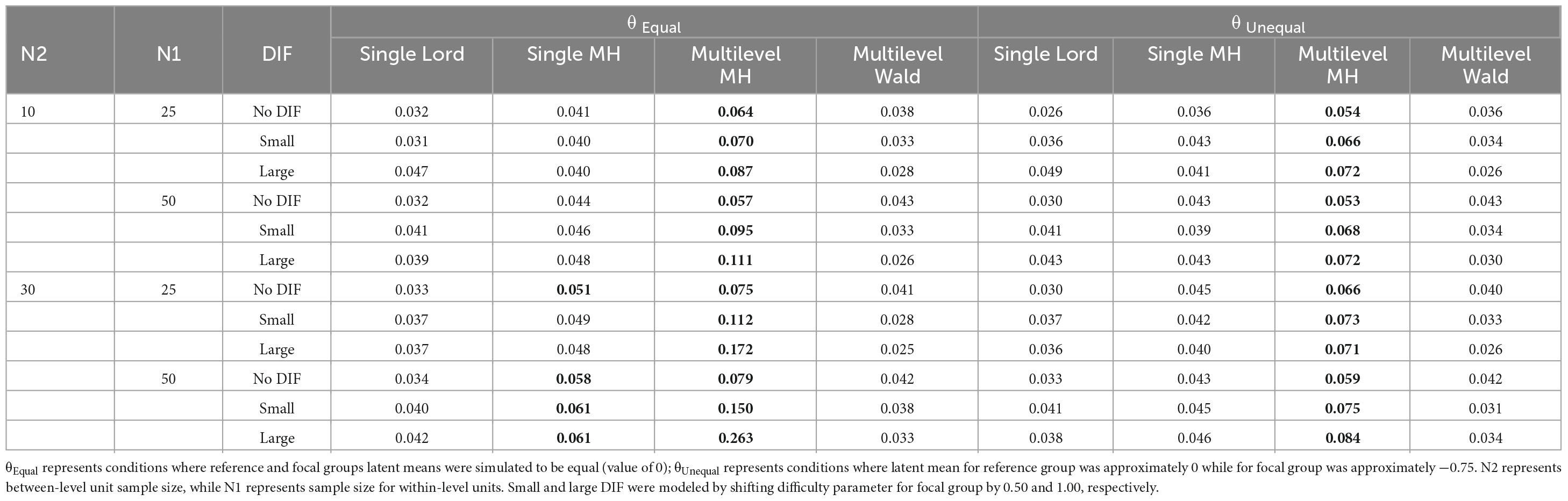
Table 2. Type I error rates across ICC and sample size ratios across between-level and within-level sample sizes for studied conditions (bolded values represent above 0.05).

FIGURE 1

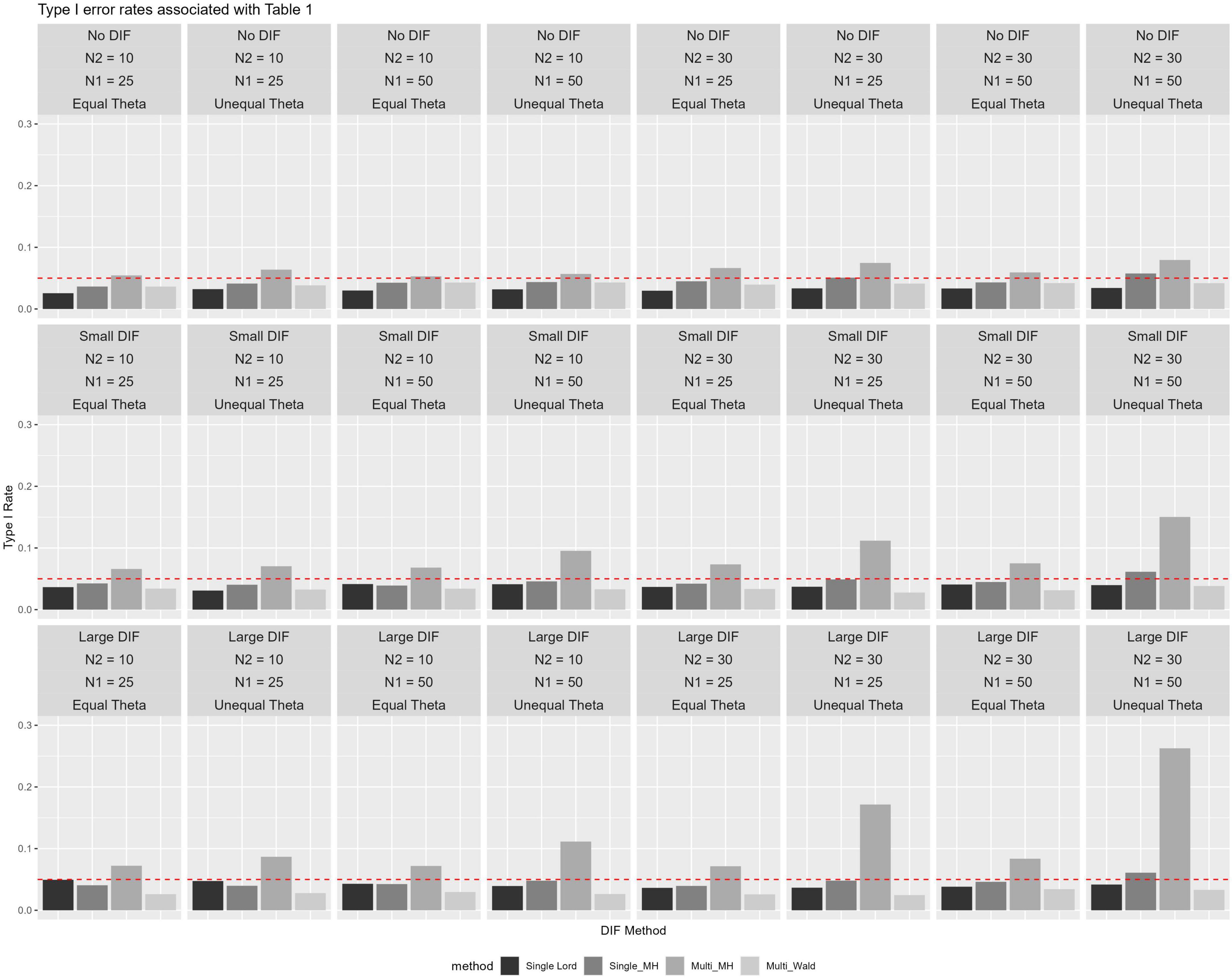
Figure 1. Type I error rates across ICC and sample size ratios across Level-2 and Level-1 sample sizes for studied conditions with 0.05 reference line.

In null conditions, Type I error rates were maintained quite well at around the 0.05 level for three of the four studied methods (see Table 2 and Figure 1). When no DIF was simulated (null conditions), only multilevel MH rates rose above 0.05 level, in particular in conditions where numbers of between-level (N2) and within-level (N1) units increased (in the range of 0.054 to 0.079). The pattern of performance was quite similar when small DIF and large DIF conditions were studied, in that multilevel MH Type I error rates were again higher across the studied conditions when compared to the other methods. For example, when small DIF was introduced, elevated Type I error rates were observed in particular for the multilevel MH method and under unequal θ conditions (i.e., when means for the two groups were different) with Type I error rates reaching 0.15 levels. When large DIF was simulated, patterns of elevated Type I error rates were similar to those previously noted, in that higher Type I error rates were found in conditions with unequal θ and a larger number of N2 and N1.

It is noteworthy that two methods, as reported in Table 2, single-level Lord and multilevel Wald test, yielded Type I error rates at or below 0.05, suggesting methods’ ability to maintain levels of false positives at a reasonable level (see “5 Discussion” for a more detailed reporting). The single-level MH method yielded rates below 0.05 across conditions, particularly those with fewer N2 and N1 and across theta levels. One exception was noted in a condition with unequal θ, and large N2 and N1, where the Type I error rate reached 0.058. Under large DIF, across studied conditions, elevated Type I error rates were observed for the multilevel MH where Type I error rates ranged from 0.071 to 0.263. Unsurprisingly, the highest rates were observed in conditions where means between the focal and reference groups were unequal (i.e., the focal group’s mean was lower by 0.75 standard deviation) and when between-level and within-level units were 30 and 50, respectively.

4.2 Power rates summary

Based on ANOVA, it was found that five of seven factors were statistically significant at the 0.05 level (i.e., N2, N1, N2/N1 ratio, method, and DIF magnitude), while two were not (ICC and θ). Post-hoc analysis suggested only one, statistically significant, pairwise comparison—single-level Lord and single-level MH. The effect sizes were large for DIF Type (${\mathrm{\eta }}_{partial}^2$ = 0.49), N2 (${\mathrm{\eta }}_{partial}^2$ = 0.45), and N1 (${\mathrm{\eta }}_{partial}^2$ = 0.22), and moderate for the method factor at = 0.07. A small ${\mathrm{\eta }}_{partial}^2$ = 0.04 was associated with N1/N2 ratio, while negligible effect sizes were found for the two remaining statistically nonsignificant main effects of θ (${\mathrm{\eta }}_{partial}^2$ = 0.001) and ICC (${\mathrm{\eta }}_{partial}^2$ < 0.001). Corresponding results for all levels of manipulated factors can be found in Supplemental materials (under Results, C1-C6).

Several observations were noted in examining results for power, as shown in Table 3 and Figure 2. Namely, across all four methods, when large DIF was introduced, high power rates were observed across all conditions. Rates of 0.80 or higher were noted, with large N2 and N1 yielding near or 1.00 power rates. The lowest power rates when DIF was large, albeit still above 0.80, were found in conditions when N2 = 10 and N1 = 25. It was only in these conditions with fewer observations at between-level and within-level that we observed some variation in methods’ performance, such that the highest power rates were observed by single-level MH, followed by multilevel MH, multilevel Wald, and single-level Lord, respectively.

TABLE 3

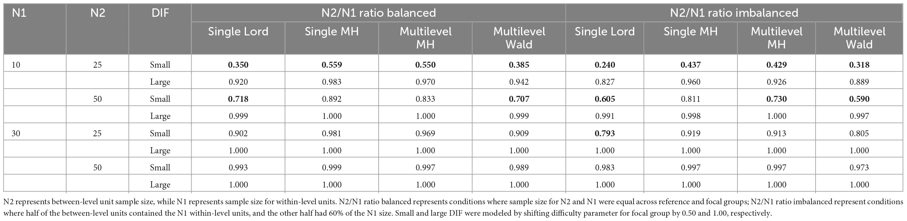
Table 3. Power rates for studied conditions averaged across ICC and theta levels (bolded values below 0.80 level).

FIGURE 2

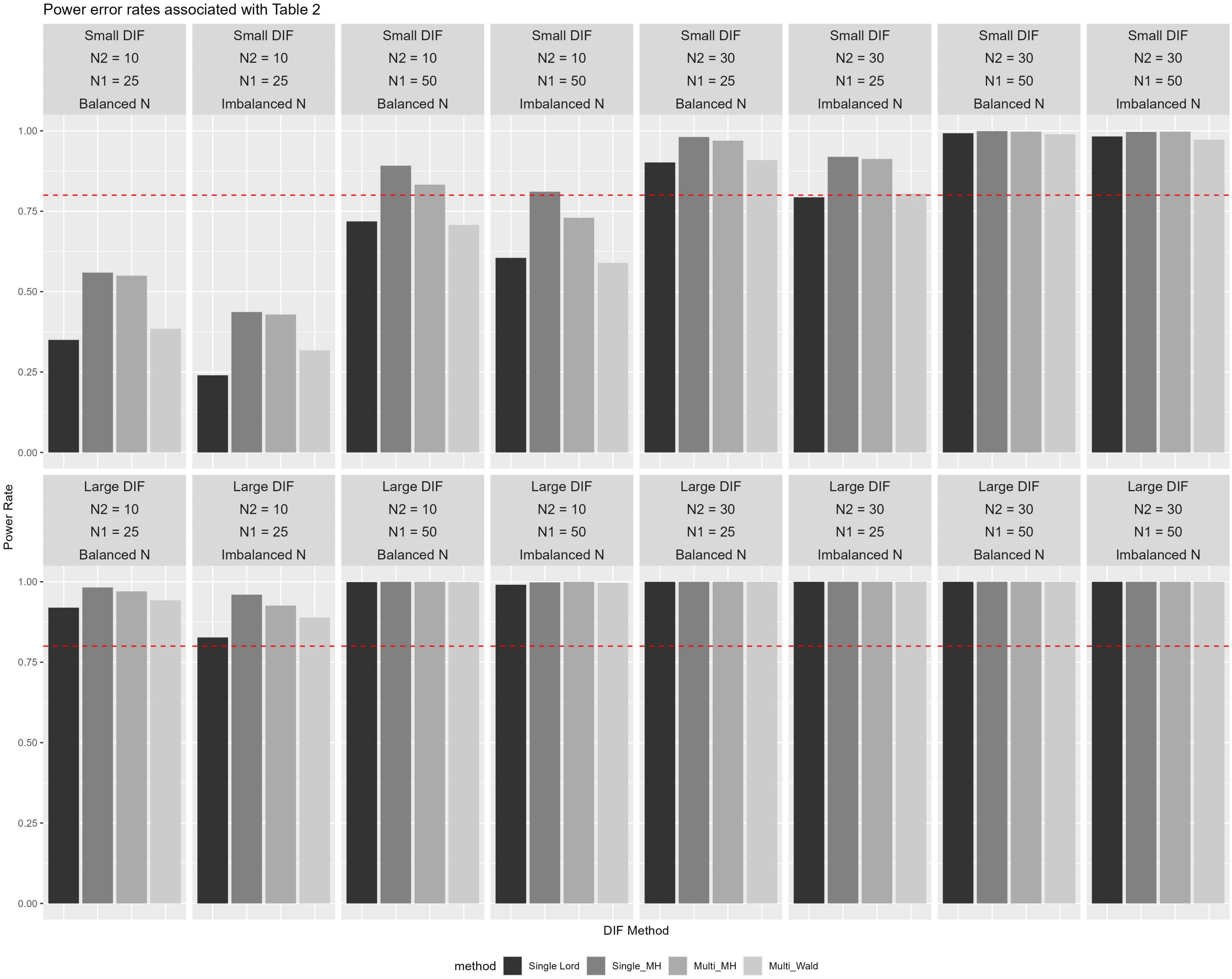
Figure 2. Power rates across ICC and theta levels for studied conditions with 0.80 reference line.

More differentiations among the methods to detect items that were simulated as DIF was found under small DIF conditions. Namely, here again we observed that the order of more powerful methods (i.e., higher observed power rates) remained similar to those in small sample sizes of large DIF conditions. Single-level MH and multilevel MH yielded the highest power rates across conditions, but to differing levels. Specifically, the power rates were considerably lower across the conditions when DIF was small for all methods. For example, in conditions with the lowest number of N2 and N1, power rates ranged from 0.350 to 0.559 for balanced and 0.240 to 0.437 for imbalanced sample sizes, respectively. As N1 increased to a sample size of 50, power rates increased to 0.590 to 0.811 for balanced and 0.707 to 0.892 for imbalanced conditions, respectively. The impact of sample balance/imbalance was observed across the conditions such that, on average, imbalanced sample sizes across N1 yielded lower power rates when compared to the balanced sample sizes, although those differences diminished as sample sizes increased.

5 Discussion

To achieve equitable measurement, identifying DIF items in an assessment is of paramount importance. While research on DIF detection methods abound, little is known about their ability in the presence of multilevel (nested) data. Given the prevalence of nested data in various social sciences (e.g., students are nested within schools; employees are nested within companies/industries), it is important to consider multilevel structures of data when conducting DIF analysis and evaluate the consequences of applying single-level methods when data are multilevel. Thus, the current study examined the performance of the four DIF detection methods in their ability to appropriately identify DIF items when data are nested. Specifically, we considered two methods that directly allow for modeling of nested data within the procedure and two routinely used single-level DIF detection methods in the score- and model-based frameworks. As such, the current study extended Magis et al. (2010) framework and provided important information for practitioners to consider when investigating DIF, in particular of their choice of the method.

A simulation study was conducted to evaluate the performance of the four DIF detection methods under various conditions when data were generated as multilevel. In addition to the aforementioned observations which were averaged across factors that yielded nonsignificant main effects and minimal effect sizes, we reflect further on the methods’ performance. As presented in Figures B1–B6 (Type I error rates) and C1-C6 (Power rates) under Results in the Supplemental materials, we observed in a more nuanced way that no one method outperformed the other three across all conditions. For example, recently proposed multilevel Wald and single-level MH had similar performance in terms of controlling Type I error rates under or around 0.05 levels across most conditions. In only two exceptions, these two methods yielded Type I error rates above 0.05. Specifically, for multilevel Wald, Type I error rates averaged above 0.05 levels (the rates were around 0.07 and 0.08) included conditions where DIF was modeled as small, N2 = 30 and N1 = 50, unequal θs with fixed ICC and imbalanced N1/N2 ratio. For single-level Lord, Type I error rates of 0.06 and 0.07 were observed only when both N2 and N1 units were small (i.e., 10 and 25, respectively), conditions with fixed ICC, when N2/N1 ratio was imbalanced and DIF was large. Similarly, as shown in Figures under Results in the Supplemental materials, power rates across various conditions tended to be the highest for single-level MH and multilevel MH methods, and differentiation among the methods was largely found in small sample sizes (N2, N1, as well as N2/N1 balanced and imbalanced ratios) when DIF was modeled as small.

In addition to the performance in detecting DIF, it is worth noting that the four studied methods vary in complexity. The two model-based methods, the single-level Lord and multilevel Wald require estimating item parameters, while the two score-based methods rely on summed scores. The multilevel Wald method consists of two stages, with an initial screening stage that uses extended Wald-2, followed by the formal evaluation stage that uses extended Wald-1. This approach is more complex and requires a researcher to have specific methodological skills when compared to, for example, a more straight forward single-level MH method. Another promising technique for selecting anchor items is Regularized Differential Item Functioning (Reg-DIF; Belzak and Bauer, 2020), which introduces a penalty function during the estimation process for anchor item selection. This model can be implemented using either frequentist (Magis et al., 2015; Robitzsch, 2023) or Bayesian (Chen and Bauer, 2023) estimation methods. Additionally, Tutz and Schauberger (2015) proposed a new penalty approach to DIF in Rasch models. Currently, it appears that neither method has been adapted to handle nested data structures. Despite this, we find the Bayesian approach especially promising. This is because Bayesian software, like Stan (Carpenter et al., 2017), seamlessly integrates with other advanced DIF detection methodologies, such as Moderated Nonlinear Factor Analysis (MNLFA; Bauer and Hussong, 2009). Furthermore, the accessibility of Bayesian approaches to IRT (Fox, 2010) has been greatly enhanced by R packages like brms (Bürkner, 2017), which enable the fitting of complex models with minimal coding effort.

Related, the accessibility of the four studied methods also varies, with three of the four methods being developed and implemented with relatively easy access within R, while multilevel Wald method requires knowledge of flexMIRT. Therefore, given the reasonably good performance of single-level methods when multilevel data are present, we recognize that it might not be necessary to always employ a more complex DIF detection method that accounts for the nested structure.

As with any simulation study, generalizability of our results and interpretations of them is bound by the choices of simulation conditions. In what follows, we discuss limitations of our study while reflecting on the future research directions. One limitation is related to the choice of our use of dichotomously scored data and the 2PL model for data generation. Namely, we studied only dichotomous items which while prevalent in educational contexts may be limiting to contexts where Likert-type items or partial credit items are used. It would be important to further study methods’ performance in polytomous scored nested data to have a more complete understanding of the impact of multilevel data on detecting DIF. We briefly reflect on that Huang and Valdivia (2023) study which introduced the novel method of multilevel Wald examined polytomously scored data, and the authors demonstrated a promise of multilevel Wald in such context. While generating item responses based on the 2PL model, the score-based MH methods were relatively disadvantaged since they use unweighted raw scores as the matching criterion. However, we did find that they perform well in many simulation conditions. Additionally, ILSAs such as PISA, use 2PL to calibrate binary scored items, further motivating our study design choices. Second, we encountered some issues in convergence which should be further studied. As noted in Appendix D, the vast majority of the methods had high levels of convergence, with over 99% of replications within conditions converged for the three methods. The lowest convergence rates, however, with an overall average of just over 82% was found in multilevel MH. While convergence was not an issue in the majority of the conditions, it was most pronounced in conditions where N2 = 10 and N1 = 25, with unequal theta, which as noted above would be something to keep in mind when analyzing data. Furthermore, we examined Monte Carlo standard errors (MCSEs) across studies outcome variables, in order to better understand our choice of 100 replications. As noted in Appendix E (Supplemental materials), we computed MCSEs and found them to be stable and comparable in size across the methods (with some variation). We also generated new data for two conditions with 1,000 replications and analyzed results for three of the four methods.⁷ The goal here was to examine whether the MCSEs would change (possibly decrease) when a much larger number of replications was considered. First selected condition yielded MCSEs based on 100 replications that were similar to the average MCSEs across the studied methods/conditions (∼0.05 and 0.36, for Type I and power, respectively). Second selected condition yielded MCSEs that were more varied across the studied methods (e.g., for Type I rate, MCSEs ranged from 0.05 to 0.10, and for power, MCSEs ranged from 0.05 to 0.15 across the methods). Both of these conditions included N2 = 10 and N = 25, with fixed ICC, while DIF and θ were different between them. As summarized in Appendix C, the results suggested very small changes when replications were increased to 1,000 compared to those found under 100 replications. Recognizing that we only examined two such conditions, and because it is a good practice, we encourage researchers to consider MCSE computation when deciding on what number of replications are desirable in the study to achieve stable results, preferably prior to conducting the analysis.

Additional limitation of the current study is related to our DIF-related factors. Because we wanted to establish impact of nested data structures on DIF detection methods, we focused on the simulation design that reflected more features related to features of data (e.g., between- and within-level units sample sizes, ICC values, etc.) rather than DIF. In addition to including other choices across the data structure factors, further attention should be given to DIF-related factors. For example, we only studied uniform DIF, and while a reasonable choice (e.g., Huang and Valdivia, 2023 found good performance of multilevel Wald in polytomous data for uniform and non-uniform DIF), it would be important to incorporate other DIF features, including non-uniform DIF. In the current study, we assumed that latent proficiency variances were equal across the groups. As Pei and Li (2010) found, latent proficiency variance had an impact on DIF detection. Thus, future research should consider examining this feature as well. Another aspect of DIF consideration concerns what is known in the literature as within- and between-DIF. Our study exclusively focused on the within-cluster DIF, as opposed to between-cluster DIF. In a multilevel data context, within-level DIF is generated at the individual level, whereas between-level DIF is generated at the cluster level. Outside a multilevel data context, most simulation studies generate DIF in a way that is analogous to the within-cluster DIF, as DIF effect sizes are typically not moderated by cluster membership. Given this, the present study focused only on within-cluster DIF, as we are most interested in research scenarios where one may reasonably consider well-established single level methods. Future research should focus on between-cluster level DIF in the presence of clustered observations, as past research has shown that this is when DIF detection methods explicitly designed for multilevel data structures are most advantageous (per French and Finch, 2010, 2013, 2015; French et al., 2019). Additionally, we only surveyed four DIF detection methods, which as one of the first studies that conducted such comparison, seems reasonable. However, we recognize that several other options exist. Thus, future researchers studying DIF in contexts of nested data might include other possible methods, such as aforementioned SIBTEST (Shealy and Stout, 1993), hierarchical logistic regression, or Bayesian approaches.

The current study provided important information to practitioners to aid the selection of DIF detection method. We recognize that aspects of the design (such as sample size) play an important role which a researcher should consider when gathering validity evidence for generalization when engaging in DIF detection analysis. For example, having larger sample size at the between-level (N2) was shown to be advantageous in detecting DIF items (i.e., generally, power rates were higher for conditions where N2 increased while keeping N1 the same, compared to analogous conditions where N1 units were increased but N2 were the same). Thinking about design, this would suggest when designing a study, a researcher might consider having larger sample size at the between-level units. We further observed that ICC levels we investigated did not seem to make a big impact on the results, which might partially explain why the single-level methods also performed quite well. Given that it was not a single method that outperformed the rest in the simulation, we recommend that researchers consider the data structure, along with additional information regarding accessibility, complexity, knowledge of the methods, when selecting any DIF detection method.

Our recommendation for applied researchers regarding which method to use when studying DIF is somewhat complex. Given the results, we cannot provide a blanket recommendation in favor of one method over another, as their performance depended on context. For example, when focusing on detecting only large DIF effects, most methods, except the multilevel MH, exhibited sufficient power and displayed appropriate Type I error rates. Multilevel MH performed particularly well (as did the other methods), yielding high power rates across conditions when sample sizes were larger. When small DIF effects were modeled, our results suggested a more complex set of recommendations is warranted. Namely, when the number of between-level units is small, the single-level MH may be the best choice as it (along with the multilevel MH) had the highest power while maintaining an acceptable Type I error rate. On the other hand, when the number of between-level units is large, either the single-level Lord or multilevel Wald is preferable as they maintain adequate power and Type I error rates.

Data availability statement

The datasets presented in this study can be found in online repositories. The names of the repository/repositories and accession number(s) can be found below: https://osf.io/96j3g/?view_only=49e6378ac0da4b4ba78b9f17949aa1c2.

Author contributions

DSV: Conceptualization, Data curation, Formal analysis, Investigation, Methodology, Software, Supervision, Validation, Visualization, Writing – original draft, Writing – review & editing. SH: Conceptualization, Formal analysis, Methodology, Software, Writing – original draft, Writing – review & editing. PB: Formal analysis, Resources, Software, Writing – original draft, Writing – review & editing.

Funding

The authors declare that financial support was received for the research, authorship, and/or publication of this article. This work was partially supported by a grant to the DSV: Indiana University Institute for Advanced Study, Indiana University—Bloomington, IN, USA. Support for open access publication charges provided by IU Libraries.

Conflict of interest

The authors declare that the research was conducted in the absence of any commercial or financial relationships that could be construed as a potential conflict of interest.

The authors declared that they were an editorial board member of Frontiers, at the time of submission. This had no impact on the peer review process and the final decision.

Publisher’s note

All claims expressed in this article are solely those of the authors and do not necessarily represent those of their affiliated organizations, or those of the publisher, the editors and the reviewers. Any product that may be evaluated in this article, or claim that may be made by its manufacturer, is not guaranteed or endorsed by the publisher.

Footnotes

1. ^ It is possible to study more than two groups in DIF analysis. In those situations, analyst selects one reference group and the remaining groups are referred to as focal groups.
2. ^ The score statistic variance, which accounts for the multilevel nature of the data, was calculated using generalized estimating equations—a method that corrects for clustered data commonly found in fields such as medicine, biology, and epidemiology (McNeish et al., 2017).
3. ^ https://osf.io/96j3g/?view_only=49e6378ac0da4b4ba78b9f17949aa1c2
4. ^ We also note that Huang and Valdivia (2023) found that ML-Wald method yielded better results (higher power rates and controlled Type I error rates) in detecting non-uniform DIF in polytomous multilevel data than uniform DIF thus motivating us to consider uniform DIF only.
5. ^ We recognize that 60% choice to create imbalance is somewhat arbitrary and that other choices are possible. Studies such as (French et al., 2019) included balanced cases, thus our efforts here are to provide initial insights into the sample size imbalance.
6. ^ Stated differently, we examined ICCs to be either equal in value (0.33) between the reference and focal groups, or varied, where varied took on two different values: ICC for reference group was set at 0.33, while for focal group at either 0.20 or 0.50.
7. ^ Due to computational time, we computed MCSEs for three of the four methods (all but multilevel Wald method), although given similarity of MCSEs when replications = 100 and 1,000 for any of the three studied methods, we would expect multilevel Wald results based on 1,000 replications to also be very consistent.

References

Bauer, D. J., and Hussong, A. M. (2009). Psychometric approaches for developing commensurate measures across independent studies: Traditional and new models. Psychol. Methods 14, 101–125. doi: 10.1037/a0015583

PubMed Abstract | Crossref Full Text | Google Scholar

Begg, M. D. (1999). Analyzing k (2×2) tables under cluster sampling. Biometrics 55, 302–307. doi: 10.1111/j.0006-341X.1999.00302.x

PubMed Abstract | Crossref Full Text | Google Scholar

Belzak, W. C. M., and Bauer, D. J. (2020). Improving the assessment of measurement invariance: Using regularization to select anchor items and identify differential item functioning. Psychol. Methods 25, 673–690. doi: 10.1037/met0000253

PubMed Abstract | Crossref Full Text | Google Scholar

Berrío, ÁI., Gomez-Benito, J., and Arias-Patiño, E. M. (2020). Developments and trends in research on methods of detecting differential item functioning. Educ. Res. Rev. 31:100340. doi: 10.1016/j.edurev.2020.100340

Crossref Full Text | Google Scholar

Bock, R. D., and Gibbons, R. D. (2021). Item response theory. Hoboken, NJ: John Wiley & Sons.

Google Scholar

Bock, R. D., and Zimowski, M. F. (1997). Multiple group IRT. Handbook of modern item response theory. New York, NY: Springer New York, 433–448.

Google Scholar

Bou Malham, P., and Saucier, G. (2014). Measurement invariance of social axioms in 23 countries. J. Cross Cult. Psychol. 45, 1046–1060.

Google Scholar

Bürkner, P. C. (2017). brms: An R package for Bayesian multilevel models using Stan. J. Stat. Softw. 80, 1–28. doi: 10.18637/jss.v080.i01

Crossref Full Text | Google Scholar

Cai, L. (2008). A Metropolis-Hastings Robbins-Monro algorithm for maximum likelihood nonlinear latent structure analysis with a comprehensive measurement model. Ph.D. thesis. Chapel Hill, NC: The University of North Carolina at Chapel Hill.

Google Scholar

Cai, L. (2010a). High-dimensional exploratory item factor analysis by a Metropolis-Hastings Robbins-Monro Algorithm. Psychometrika 75, 33–57.

Google Scholar

Cai, L. (2010b). Metropolis-Hastings Robbins-Monro algorithm for confirmatory item factor analysis. J. Educ. Behav. Stat. 35, 307–335.

Google Scholar

Cai, L. (2017). Flexible multilevel multidimensional item analysis and test scoring [computer software]; flexMIRT R version 3.51. Chapel Hill, NC: Vector Psychometric Group.

Google Scholar

Cai, L., Thissen, D., and du Toit, S. H. C. (2011). IRTPRO: Flexible, multidimensional, multiple categorical IRT modeling [computer software]. Lincolnwood, IL: Scientific Software International.

Google Scholar

Candell, G. L., and Drasgow, F. (1988). An iterative procedure for linking metrics and assessing item bias in item response theory. Appl. Psychol. Meas. 12, 253–260. doi: 10.1177/014662168801200304

Crossref Full Text | Google Scholar

Carpenter, B., Gelman, A., Hoffman, M. D., Lee, D., Goodrich, B., Betancourt, M., et al. (2017). Stan: A probabilistic programming language. J. Stat. Softw. 76, 1–32. doi: 10.18637/jss.v076.i01

PubMed Abstract | Crossref Full Text | Google Scholar

Chen, S. M., and Bauer, D. J. (2023). Modeling growth in the presence of changing measurement properties between persons and within persons over time: A Bayesian regularized second-order growth curve model. Multiv. Behav. Res. 58, 150–151. doi: 10.1080/00273171.2022.2160955

PubMed Abstract | Crossref Full Text | Google Scholar

Cook, L. L., and Eignor, D. R. (1991). IRT equating methods. Educ. Meas. Issues Pract. 10, 37–45. doi: 10.1111/j.1745-3992.1991.tb00207.x

Crossref Full Text | Google Scholar

Dai, S., French, B. F., Finch, W. H., Iverson, A., and Dai, M. S. (2022). Package ‘DIFplus’. R package version 1.1. Available online at: https://CRAN.R-project.org/package=DIFplus (accessed October 12, 2023).

Google Scholar

Economic Co-operation and Development (2010). TALIS technical report. Paris: Economic Co-operation and Development.

Google Scholar

Fox, J. P. (2010). Bayesian item response modeling: Theory and applications. New York, NY: Springer.

Google Scholar

French, B. F., and Finch, W. H. (2010). Hierarchical logistic regression: Accounting for multilevel data in DIF detection. J. Educ. Meas. 47, 299–317. doi: 10.1111/j.1745-3984.2010.00115.x

Crossref Full Text | Google Scholar

French, B. F., and Finch, W. H. (2013). Extensions of Mantel–Haenszel for multilevel DIF detection. Educ. Psychol. Meas. 73, 648–671. doi: 10.1177/0013164412472341

Crossref Full Text | Google Scholar

French, B. F., and Finch, W. H. (2015). Transforming SIBTEST to account for multilevel data structures. J. Educ. Meas. 52, 159–180.

Google Scholar

French, B. F., Finch, W. H., and Immekus, J. C. (2019). Multilevel generalized Mantel-Haenszel for differential item functioning detection. Front. Educ. 4:47. doi: 10.3389/feduc.2019.00047

Crossref Full Text | Google Scholar

French, B. F., Finch, W. H., and Vazquez, J. A. V. (2016). Differential item functioning on mathematics items using multilevel SIBTEST. Psychol. Test Assess. Model. 58:471.

Google Scholar

Gao, X. (2019). A comparison of six DIF detection methods. Master’s thesis. Available online at: https://opencommons.uconn.edu/gs_theses/1411

Google Scholar

Guilera, G., Gómez-Benito, J., Hidalgo, M. D., and Sánchez-Meca, J. (2013). Type I error and statistical power of the Mantel-Haenszel procedure for detecting DIF: A meta-analysis. Psychol. Methods 18:553. doi: 10.1037/a0034306

PubMed Abstract | Crossref Full Text | Google Scholar

Hagger, M., Biddle, S., Chow, E., Stambulova, N., and Kavussanu, M. (2003). Physical self-perceptions in adolescence: Generalizability of a hierarchical multidimensional model across three cultures. J. Cross Cult. Psychol. 34, 611–628.

Google Scholar

Hansen, M., Cai, L., Stucky, B. D., Tucker, J. S., Shadel, W. G., and Edelen, M. O. (2014). Methodology for developing and evaluating the PROMIS_ smoking item banks. Nicotine Tobacco Res. 16, S175–S189.

Google Scholar

Holland, P. W., and Thayer, D. T. (1988). “Differential item performance and the Mantel-Haenszel procedure,” in Test validity, eds H. Wainer and H. I. Braun (Lawrence Erlbaum Associates, Inc), 129–145.

Google Scholar

Holland, P. W., and Wainer, H. (2012). Differential item functioning. New York, NY: Routledge.

Google Scholar

Huang, S., and Valdivia, D. S. (2023). Wald χ2 test for differential item functioning detection with polytomous items in multilevel data. Educ. Psychol. Meas. doi: 10.1177/00131644231181688

Crossref Full Text | Google Scholar

Jin, Y., Myers, N. D., and Ahn, S. (2014). Complex versus simple modeling for DIF detection: When the intraclass correlation coefficient (r) of the studied item is less than the r of the Total score. Educ. Psychol. Meas. 74, 163–190. doi: 10.1177/0013164413497572

Crossref Full Text | Google Scholar

Joo, S., Valdivia, M., Valdivia, D. S., and Rutkowski, L. (2023). Alternatives to weighted item fit statistics for establishing measurement invariance in many groups. J. Educ. Behav. Stat. doi: 10.3102/10769986231183326

PubMed Abstract | Crossref Full Text | Google Scholar

Jöreskog, K. G. (1971). Simultaneous factor analysis in several populations. Psychometrika 36, 409–426. doi: 10.1007/BF02291366

Crossref Full Text | Google Scholar

Langer, M. M. (2008). A reexamination of Lord’s Wald test for differential item functioning using item response theory and modern error estimation Ph.D. thesis. Chapel Hill, NC: The University of North Carolina at Chapel Hill.

Google Scholar

Liu, X. (2024). Detecting differential item functioning with multiple causes: A comparison of three methods. Int. J. Test. 24, 53–59. doi: 10.1080/15305058.2023.2286381

Crossref Full Text | Google Scholar

Lord, F. M. (1980). Applications of item response theory to practical testing problems. Lawrence Erlbaum.

Google Scholar

Magis, D., Beland, S., Tuerlinckx, F., and De Boeck, P. (2010). A general framework and an R package for the detection of dichotomous differential item functioning. Behav. Res. Methods 42, 847–862. doi: 10.3758/BRM.42.3.847

PubMed Abstract | Crossref Full Text | Google Scholar

Magis, D., Tuerlinckx, F., and Destaeck, P. (2015). Detection of differential item functioning using the lasso approach. J. Educ. Behav. Stat. 40, 111–135. doi: 10.3102/1076998614559747

PubMed Abstract | Crossref Full Text | Google Scholar

Mantel, N., and Haenszel, W. (1959). Statistical aspects of the analysis of data from retrospective studies of disease. J. Natl. Cancer Inst. 22, 719–748. doi: 10.1093/jnci/22.4.719

Crossref Full Text | Google Scholar

Marsh, H. W., Abduljabbar, A. S., Morin, A. J. S., Parker, P., Abdelfattah, F., Nagengast, B., et al. (2015). The big-fish-little-pond effect: Generalizability of social comparison processes over two age cohorts from Western, Asian, and Middle Eastern Islamic countries. J. Educ. Psychol. 107, 258–271. doi: 10.1037/a0037485

Crossref Full Text | Google Scholar

Marsh, H. W., Lüdtke, O., Nagengast, B., Trautwein, U., Morin, A. J., Abduljabbar, A. S., et al. (2012). Classroom climate and contextual effects: Conceptual and methodological issues in the evaluation of group-level effects. Educ. Psychol. 47, 106–124. doi: 10.1080/00461520.2012.670488

Crossref Full Text | Google Scholar

McNeish, D., Stapleton, L. M., and Silverman, R. D. (2017). On the unnecessary ubiquity of hierarchical linear modeling. Psychol. Methods 22:114. doi: 10.1037/met0000078

PubMed Abstract | Crossref Full Text | Google Scholar

Megreya, A. M., Latzman, R. D., Al-Attiyah, A. A., and Alrashidi, M. (2016). The robustness of the nine-factor structure of the cognitive emotion regulation questionnaire across four arabic speaking middle eastern countries. J. Cross-Cult. Psychol. 47, 875–890. doi: 10.1177/0022022116644785

Crossref Full Text | Google Scholar

Meredith, W. (1993). Measurement invariance, factor analysis and factorial invariance. Psychometrika 58, 525–543. doi: 10.1007/BF02294825

Crossref Full Text | Google Scholar

Muthen, B. O. (1994). Multilevel covariance structure analysis. Sociol. Methods Res. 22, 376–398.

Google Scholar

Narayanon, P., and Swaminathan, H. (1996). Identification of items that show nonuniform DIF. Appl. Psychol. Meas. 20, 257–274. doi: 10.1177/014662169602000306

Crossref Full Text | Google Scholar

Olson, J., Martin, M. O., and Mullis, I. V. S. (2008). TIMSS 2007 technical report. Chestnut Hill, MA: TIMSS & PIRLS International Study Center, Boston College.

Google Scholar

Ozel, M., Caglak, S., and Erdogan, M. (2013). Are affective factors a good predictor of science achievement? Examining the role of affective factors based on PISA 2006. Learn. Individ. Differ. 24, 73–82. doi: 10.1016/j.lindif.2012.09.006

Crossref Full Text | Google Scholar

Pei, L. K., and Li, J. (2010). Effects of unequal ability variances on the performance of logistic regression, Mantel-Haenszel, SIBTEST IRT, and IRT likelihood ratio for DIF detection. Appl. Psychol. Meas. 34, 453–456.

Google Scholar

Penfield, R. D. (2001). Assessing differential item functioning among multiple groups: A comparison of three Mantel-Haenszel procedures. Appl. Meas. Educ. 14, 235–259. doi: 10.1207/S15324818AME1403_3

Crossref Full Text | Google Scholar

Peugh, J. L. (2010). A practical guide to multilevel modeling. J. Sch. Psychol. 48, 85–112. doi: 10.1016/j.jsp.2009.09.002

PubMed Abstract | Crossref Full Text | Google Scholar

R Core Team (2023). R: A language and environment for statistical computing. Vienna: R Foundation for Statistical Computing.

Google Scholar

Robitzsch, A. (2023). Comparing robust linking and regularized estimation for linking two groups in the 1PL and 2PL models in the presence of sparse uniform differential item functioning. Stats 6, 192–208. doi: 10.3390/stats6010012

Crossref Full Text | Google Scholar

Roussos, L. A., Schnipke, D. L., and Pashley, P. J. (1999). A generalized formula for the Mantel-Haenszel differential item functioning parameter. J. Educ. Behav. Stat. 24, 293–322. doi: 10.3102/10769986024003293

PubMed Abstract | Crossref Full Text | Google Scholar

Rubin, D. B. (1981). Estimation in parallel randomized experiments. J. Educ. Stat. 6, 377–401. doi: 10.3102/10769986006004377

PubMed Abstract | Crossref Full Text | Google Scholar

Segeritz, M., and Pant, H. A. (2013). Do they feel the same way about math?: Testing measurement invariance of the PISA “students’ approaches to learning” instrument across immigrant groups within Germany. Educ. Psychol. Meas. 73, 601–630. doi: 10.1177/0013164413481802

Crossref Full Text | Google Scholar

Shealy, R., and Stout, W. (1993). A model-based standardization approach that separates true bias/DIF from group ability differences and detects test bias/DTF as well as item bias/DIF. Psychometrika 58, 159–194. doi: 10.1007/BF02294572

Crossref Full Text | Google Scholar

Sulis, I., and Toland, M. D. (2017). Introduction to multilevel item response theory analysis: Descriptive and explanatory models. J. Early Adolesc. 37, 85–128. doi: 10.1177/0272431616642328

Crossref Full Text | Google Scholar

Svetina, D., and Rutkowski, L. (2014). Detecting differential item functioning using generalized logistic regression in the context of large-scale assessments. Large Scale Assess. Educ. 2, 1–17. doi: 10.1186/s40536-014-0004-5

Crossref Full Text | Google Scholar

Szabo, A., Ward, C., and Fletcher, G. O. (2016). Identity processing styles during cultural transition: Construct and measurement. J. Cross Cult. Psychol. 47, 483–507. doi: 10.1177/0022022116631825

Crossref Full Text | Google Scholar

Tutz, G., and Schauberger, G. (2015). A penalty approach to differential item functioning in Rasch models. Psychometrika 80, 21–43. doi: 10.1007/s11336-013-9377-6

PubMed Abstract | Crossref Full Text | Google Scholar

Yates, F. (1934). Contingency tables involving small numbers and the χ 2 test. Suppl. J. R. Stat. Soc. 1, 217–235.

Google Scholar