Statistical Analysis Based Feature Selection Enhanced RF-PUF With >99.8% Accuracy on Unmodified Commodity Transmitters for IoT Physical Security

1 Introduction

The fourth industrial revolution, fueled by low-power, high-speed modern communication systems has ushered in a new era of immersive and unprecedented user experience through smart devices. These devices are connected not only with each other but also to the cloud and are popularly known as the Internet of Things (IoT). The global IoT market is experiencing a rapid boost and according to a prediction by Norton, there will be around 21 billion connected devices by 2025 (Symanovich 2019). Researchers are already talking about the Internet of Everything (IoE) which essentially refers to people, data, and smart things connected to form an ecosystem that ensures a better and smarter lifestyle. The diverse application environment of the smart devices has rendered them vulnerable to a wide attacking surface. The weakest point in a network defines its overall security. The resource-limited, user-end devices are the weakest nodes of the IoT networks where a security compromise can provide access to a rogue device that can pose a massive threat to all the connected nodes and user data. So, the question of secure authentication before granting access to a large network is of increasing importance.

Traditional methods such as symmetric-key cryptography and asymmetric-key cryptography use secret private keys or public/private key pairs respectively, for encryption/decryption. Key-based methods require the storage of a secret key in a nonvolatile memory (NVM) or SRAM. However, they are vulnerable to different invasive/semi-invasive key-hacking attacks and side-channel attacks (Kocher et al., 1999; Quisquater and Samyde 2001; Hospodar et al., 2011). Multi-factor authentication (MFA) (Ting et al., 2015; Ometov et al., 2018) requires one or more verification factors (e.g., biometric factor, two-factor code from authentication app, etc.) along with the secret key. The widely-used open authentication (OAuth 2.0) protocol (OAuth 2.0 and OAuth 2022) for current IoT networks suffers from cross-site request forgery (CSRF) attacks (Barth et al., 2008; Siddiqui and Verma 2011). Both OAuth and MFA are inconvenient for large networks as they require manual verification. In addition to these vulnerabilities, the use of digital signatures also puts additional power and area burden which are typically small but could be significant for extremely energy and resource constraint edge devices.

To circumvent this, the idea of radio frequency physical unclonable function (RF-PUF) has been recently proposed (Chatterjee et al., 2019) using physical signature instead of or in addition to the digital signature. The concept of RF-PUF is explained in Figure 1. RF-PUF exploits the inherent device imperfections due to manufacturing process variation and other system-level nonidealities (e.g., LO frequency offset, I-Q mismatch, DC offset, attenuation, fading, Doppler shift, etc.) as unique physical signatures. These signatures are used as features and fed to a neural network at the receiver to train it. Once trained, this network can be employed at the receiver for authentication. RF-PUF does not demand any additional preamble, digital keys, or assistive communication medium for authentication purposes. The absence of an external security key or preamble makes RF-PUF highly resilient to different types of key-hacking attacks and alleviates the need for preamble obfuscation (Chacko 2017). Also, it does not require any secured memory block for key storage. Thus, both power and area overhead is reduced on the resource-constrained edge-node side of an asymmetric IoT network.

FIGURE 1

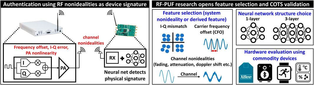
FIGURE 1. The concept of RF-PUF exploits the inherent physical signature embedded in the device which manifests itself as different imperfections, which are used as features to train a neural network at the receiver end for authentication. The challenges involve developing a proper feature set, choosing a proper neural network architecture, and evaluating the concept in real, commodity devices.

In (Chatterjee et al., 2019), the idea of RF-PUF was presented primarily based on simulation data using I-Q samples as features. However, the PUF output is stochastic in nature and it is very hard to accurately capture the device nonidealities in simulation. This calls for addressing the open research needs of experimental validation of RF-PUF and demonstration of high-accuracy on devices found ‘in-the-wild’. In this work, we address both these research problems by 1) analyzing the efficacy of RF-PUF on unmodified commodity devices and 2) introducing effective feature selection to increase RF-PUF accuracy $>99.8\%$. To achieve this, an improved and robust feature set is necessary to provide a reliable authentication method. We purchased commercially available 30 Xbee S2C devices and used them as unmodified commodity COTS (Components off-the-self) devices to experimentally validate RF-PUF. 155.4 GB of data have been collected from the Xbee transceiver systems and 2.5 GB of data have been used for experimentation. This dataset has also been made public on GitHub along with this paper, for further development and validation by the RF-Security community.

It has been shown that 95% accuracy can be achieved even with a lightweight, single-layer neural network with 10 neurons and $\sim 1.8$ ms (30 kB) of test data, which ensures the feasibility of RF-PUF in a low-latency network. With statistical analysis, a new feature has been augmented that massively boosts the performance of the network. The impact of the variation in neural network model capacity and the amount of training data on detection accuracy has been explored. Along with artificial neural networks, experiments have been performed with multiple traditional machine learning algorithms, and their performance is compared in terms of the number of devices. A detailed analysis of the PUF properties has been done to evaluate the eligibility of RF-PUF as a PUF. Inter-PUF and intra-PUF hamming distances have been calculated and it has been proved that for commodity COTS (Components off-the-self) devices without any modification, RF-PUF shows strong identifiability with a very high (99.87%) detection probability. As an authentication method, possible vulnerabilities and attack models for RF-PUF have been investigated and the robustness of RF-PUF against them has been proved. The insights gathered from these analyses and experiments may prove to be extremely important for the design and implementation of RF-PUF in the future in realistic application scenarios with “in-the-wild” devices.

1.1 Our Contribution

In this work, through thorough statistical analysis of unmodified commodity devices, we have found an optimum feature that improves the accuracy of RF-PUF significantly on a suite of commodity hardware devices leading to $>$ 99.8% accuracy, along with PUF property analysis and security vulnerability analysis. Detailed contributions are as follows:

(1) Feature engineering: Principal component analysis has been performed on the existing feature set found in the literature to find the dominant feature. Through moment analysis on the dominant feature (i.e. carrier frequency offset) we demonstrate that the addition of a feature called COV (ratio of standard deviation and mean of carrier frequency offset) significantly helps in achieving high $(>99.8\%)$ accuracy (Section 4.3).

(2) Highest accuracy achieved with unmodified COTS devices: 30 Xbee S2C modules have been used without the help of any assisting communication preamble or any modification to the devices whatsoever. Using data received over a wireless channel with a suitable feature set and a lightweight neural network, 99.8% accuracy can be achieved which, to our best knowledge, is the highest accuracy using this many commodity COTS devices considering the wireless channel (Section 4.4).

(3) RF-PUF established as a strong PUF: Any distinct PUF class is identified through some properties that make it a separate class. They include constructability, evaluability, uniqueness, reliability, and identifiability. We have explored these properties for RF-PUF in detail, calculated intra-PUF and inter-PUF hamming distances and in an extensive test of 41238000 cases, we have shown that the probability of proper identification of an RF-PUF instance is 0.9987. This is the first time analysis of RF-PUF as a PUF class which experimentally demonstrates RF-PUF as a strong and unique PUF class by itself (Section 6).

(4) Performance evaluation using popular machine learning algorithms and comparison with neural network (NN) based approach. It has been shown that even a lightweight NN with a single hidden layer can handle $>$300 devices with 99.9% accuracy, unlike ML algorithms (Section 5.4).

(5) Wireless channel variability analysis on the accuracy of RF-PUF and the effect of network depth on accuracy with and without a wireless channel has been presented. Discussion on possible important attack models and the robustness of RF-PUF against such attacks (Section 5.5).

(6) Public Dataset: Our collected data have been released as a public dataset for the whole community to explore and experiment with (Section 3.3).

The rest of the paper is structured as follows: Section 2 provides relevant works on RF fingerprinting and device authentication. Section 3 provides an overview of our experimental setup, data collection, and data processing method. Section 4 presents a new feature set development using statistical analysis and corresponding performance enhancement. Section 5 explores the design space in detail. Section 6 analyzes various PUF properties in the context of RF-PUF. Section 7 discusses possible attack models and the resilience of RF-PUF against them. Finally, section 8 concludes this paper.

2 Related Works

Traditional RF fingerprinting approaches use modulation domain metrics, statistical parameters, transient properties, wavelet-based approaches, etc. In (Brik et al., 2008), authors used various modulation domain metrics such as frequency and IQ offset, magnitude and phase error, sync correlation, etc. to propose a radio device identification method called PARADIS (PAssive RAdiometic Device Identification System). They collected data from 138 Atheros network interface cards (NIC) and tested their proposed methods (SVM-based and kNN-based) on the ORBIT testbed facility (ORBIT 2022). They achieved an error rate of 3% for 138 NIC classification. In (Zhuo et al., 2017) authors have used IQ imbalance-based features for device fingerprinting. Based on simulation data from 5 transmitters and 400 signals from each of them, they have shown that they can achieve $>$90% accuracy for SNR ≥ 15 dB and $>$99% accuracy for SNR ≥ 20 dB. Authors in (Danev et al., 2009) have used modulation shape and spectral features to identify RFIDs (Radio Frequency Identification Devices). They collected data from 50 JCOP NXP 4.1 smart cards and 8 e-passports and matched the extracted fingerprints with the reference using standardized Euclidean distances. For 50 RFIDs, they achieved 95% accuracy when spectral features are used standalone and 97.5% accuracy when the features are combined. In (Huang and Zheng 2012), authors have used constellation deviation from ideal constellation as features. This work is similar to previously mentioned works in the sense that constellation error contains information about IQ imbalances, magnitude and phase error, etc. They collected data from 7 TDMA satellites for testing and achieved an accuracy of $>$95%.

Several fingerprinting methods use transients during device start-up and extract features from them. But before feature extraction, proper detection of the transients is a major challenge and several approaches for that are described in (Shaw and Kinsner 1997; Hall et al., 2003). Authors in (Danev and Capkun 2009) have used data from 50 COTS devices (Tmote Sky sensor) and FFT-based Fisher features to show an accuracy of $>$99%. An interesting approach was described in (Yuan et al., 2014) where authors calculated energy distribution of transients in time and frequency domain using Hilbert-Huang Transform (Huang 2014) which uses IMFs in EMD (Bari and Anowarul Fattah 2020) with Hilbert transform. However, their dataset was very small, consisting of 8 GSM mobile phones used as transmitters. Similar work was proposed in (Ur Rehman et al., 2012), where authors calculated energy envelopes for Bluetooth devices. Their dataset was also small, containing only 7 Bluetooth devices. In this small dataset, they could achieve 99.9% accuracy. Some wavelet-based approaches have also been used in literature. For example, authors in (Klein et al., 2009) have used DT-CWT (dual-tree complex wavelet transform) based features to fingerprint RF devices. At low SNR (8dB), they could achieve 80% accuracy. Authors in (Bertoncini et al., 2012) have used dynamic wavelet fingerprints to classify 146 RFID devices. They used four types of classifiers (LDC, QDC, k-NN, and SVM) and achieved 99% accuracy. Another work (Kennedy et al., 2008) involved frequency domain analysis with a k-NN classifier which achieved 97% accuracy at 30 dB SNR.

There are other works that have used various time and frequency domain properties of individual transmitters for RF fingerprinting (Rasmussen and Capkun 2007; Scanlon et al., 2010; Nguyen et al., 2011; Bihl et al., 2016; Vo-Huu et al., 2016; Peng et al., 2018; Xie et al., 2018). However, both time and frequency domain analysis have their limitations in the form of detecting the start and end of the transients, high oversampling ratios, and the need for fixed preambles to avoid data dependency. MAC layer and other upper layers of the communication protocol have also been used for RF-fingerprinting (Xu et al., 2016a). However, device identifiers in upper layers like IMEI number, IP address, MAC address, etc. can be spoofed (Chomsiri 2007; Kumar et al., 2015; Alotaibi and Elleithy 2016; Wang and Yang 2017). Several statistical parameter-based approaches have also been proposed. For example, authors in (Patel 2015) have used various statistical features to identify 4 Xbee devices. Using a Random Forrest classifier (Pal 2005), they could achieve 97% accuracy for SNR ≥ 10 dB. Another work (Lukacs et al., 2015) has used RF-DNA (Radio Frequency Distinct Native Attribute) dependent RF fingerprinting. RF-DNA uses various statistical features. For a 7 class dataset, authors have achieved an average accuracy of 81% for the MDA/ML classifier. For real-time device authentication, authors in (Bari et al., 2021a) have used a dynamic irregular clustering approach. One attractive feature here is that this algorithm learns incrementally with more input data.

Recently deep learning-based RF fingerprinting has gained popularity. Different types of deep networks (convolutional neural networks or CNN (Albawi et al., 2017; Kim 2017), recurrent neural network or RNN (Medsker and Jain 2001; Liu et al., 2016), generative adversarial networks or GAN (Mao et al., 2017; Creswell et al., 2018), etc.) are being used extensively for RF device identification and authentication. Hanna et al. utilized power amplifier nonlinearity with deep learning to fingerprint RF devices (Hanna and Cabric 2019) using simulation data. In (Sankhe et al., 2020), authors proposed a new method called ORACLE (Optimized Radio clAssification through Convolutional neuraL nEtworks) using the AlexNet-like CNN framework. With data from 16 USRP X310 transmitters, they could achieve 87.13 and 99% accuracy for the static and quasi-static channels respectively. However, wireless data are contaminated with noise and interference, any use of the RF data without processing always posits a risk of huge performance drop in scenarios where environmental nonidealities can go beyond the estimation that was used while designing the network. Processing data, extracting a proper feature set, and unraveling the mystery of the design space can render a robust authentication method that is less vulnerable to environmental factors and provides more flexibility to the designer. That is why RF-PUF performs better than the CNN-based approach as shown in (Bari et al., 2021b). In (Soltani et al., 2020), authors have used multiple deep networks and integrated their outputs to make a final prediction. They collected data from 7 UAVs or drones (DJI M100) and got maximum accuracy of 99% with data augmentation. Using data from 5 USRP devices and bispectrum of the received signal as the feature, authors in (Ding et al., 2018) have achieved 75% accuracy with a custom CNN. Another work (Peng et al., 2020) also used custom CNN with DCTF (Differential Constellation Trace Figure) as features to fingerprint 16 Xbee devices. For SNR ≥ 15 dB, they achieved 90% accuracy. In (Zong et al., 2020), authors have used CNN to identify 5 transmitter devices. Although they achieved 99% accuracy, their dataset is quite small.

A much bigger and more extensive dataset is the DARPA RFMLS dataset, containing data from 10000 devices (Jian et al., 2020). The authors have presented two architecture based on AlexNet and ResNet-50 to perform multiple learning tasks. On this dataset, another group of researchers has used a modified CNN called ADCC (augmented dilated causal convolution network) (Robinson et al., 2020). Apart from these traditional or modified CNN-based methods, there are some works reported in the literature that use GAN. For example, AC-WGAN (Auxiliary Classifier Wasserstein Generative Adversarial Networks) achieves 95% accuracy for UAV classification (Zhao et al., 2018). For a low number of devices (8 USRP B210), authors have achieved 99.9% accuracy using GAN (Roy et al., 2019). Some other prominent works for RF fingerprinting using deep learning are mentioned in (O’Shea and Hoydis 2017; Wang et al., 2017; Wang et al., 2018; Zhang et al., 2019). A detailed review of RF fingerprinting methods can be found in (Xu et al., 2016b; Guo et al., 2019; Jagannath et al., 2022). Our experimental study in this work shows $>$99.8% detection accuracy which is better than almost all the studies mentioned above. Only a few have achieved 99.9% accuracy, but with a much smaller dataset (containing less than 10 devices) compared to our dataset of 30 devices.

3 Experimental Setup

3.1 Physical Device Setup

For experimental validation, 30 XBee S2C modules are chosen (IEEE 802.15.4 standard) which is designed for industrial and commercial use. Figure 2A shows the Xbee devices whereas Figure 2B, and Figure 2C show the block diagram and the actual setup. The TX and RX are kept 1 m apart. Using SMA cable, a HackRF One software-defined radio (SDR) module has been connected either to the TX (case 1) or to the RX (case 2) to extract data excluding (case 1) or including (case 2) wireless channel.

FIGURE 2

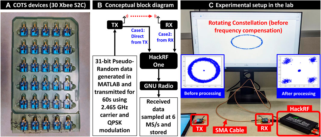
FIGURE 2. (A) Commodity off-the-shelf devices (30 Xbee S2C modules) used as transmitters for data collection. (B) Conceptual experimental setup. (C) Actual experimental setup in the lab. The TX and RX are placed 1 m apart (they are close here for image capturing purposes only) and a HackRF module was used to collect data either from the TX (case 1) or RX (case 2). GNU Radio records the collected data and shows a live constellation (visible on-screen). The rotating constellation is later processed in MATLAB through coarse and fine frequency compensation.

3.2 Data Collection and Filtering Noise

A 31-bit pseudo-random bit sequence (PRBS) is generated in MATLAB and fed to each TX which transmits this data for 60 s with QPSK modulation at 2.465 GHz and 230,400 bps baud rate. These data were captured in a Xbee RX module. Simultaneously, data were also captured by a HackRF one software-defined radio (SDR) module, sampled at 6 MSps, and stored by GNU Radio. The captured data are divided into several frames, each containing a number of samples. From the constellation diagram of the frame data (Figure 3), it is found that some frames have no significant data points and contain only noise as the Xbee devices transmit data intermittently due to their buffer limitation. These blank frames containing only noise were discarded.

FIGURE 3

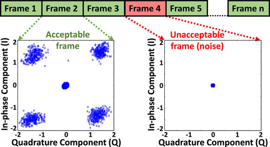
FIGURE 3. Grouping collected data in a number of frames and filtering of data for acceptable frames. This step is required as the Xbee module transmits data on an interval.

3.3 Public Dataset

This dataset contains raw data collected from 30 Xbee S2C transmitters for both cases (excluding and including the channel) in binary format. The total size of the dataset is 155.4 GB (each transmitter data is ∼2.5 GB). It can be downloaded from Sparclab RF-PUF Dataset (Bari and Sen 2022).

4 Feature Extraction

4.1 Initial Feature Set

In our work, CFO and I-Q data are taken as features just as in the original RF-PUF paper (Chatterjee et al., 2019). The previously generated frames are filtered using matched filtering, frequency compensated (both fine and coarse), and finally synchronized using timing recovery. In this process, CFO is found as a byproduct. Along with CFO, the compensated in-phase and quadrature-phase components in four quadrants are used as features. The 9 features (CFO + 4 I-components + 4 Q-components) from each frame and 1,000 frames from each TX lead to a feature set of 9 × 1000. The final feature matrix is a combination of these feature sets from all 30 devices and has a size of 9 × 30000.

4.2 Accuracy With Carrier Frequency Offset and I-Q Features

The whole feature data are divided into 70%, 15%, and 15% respectively for training, validation, and test purposes and fed into a neural network (NN). The performance of the neural network is tested by varying the number of neurons and hidden layers. Figure 4A shows the accuracy of the trained model for different neural networks. The accuracy is less than 75% in all test cases. Since exploring different NN configurations does not provide expected accuracy, our choice here is to: 1) form an improved feature set to be used with the NN 2) use different machine learning (ML) algorithms 3) use more data. We first search for an improved feature set for better accuracy. Later, the effect of more data is shown in subsection 5.1, 5.2 and a comparison of different ML algorithms and NN is discussed in subsection 5.4.

FIGURE 4

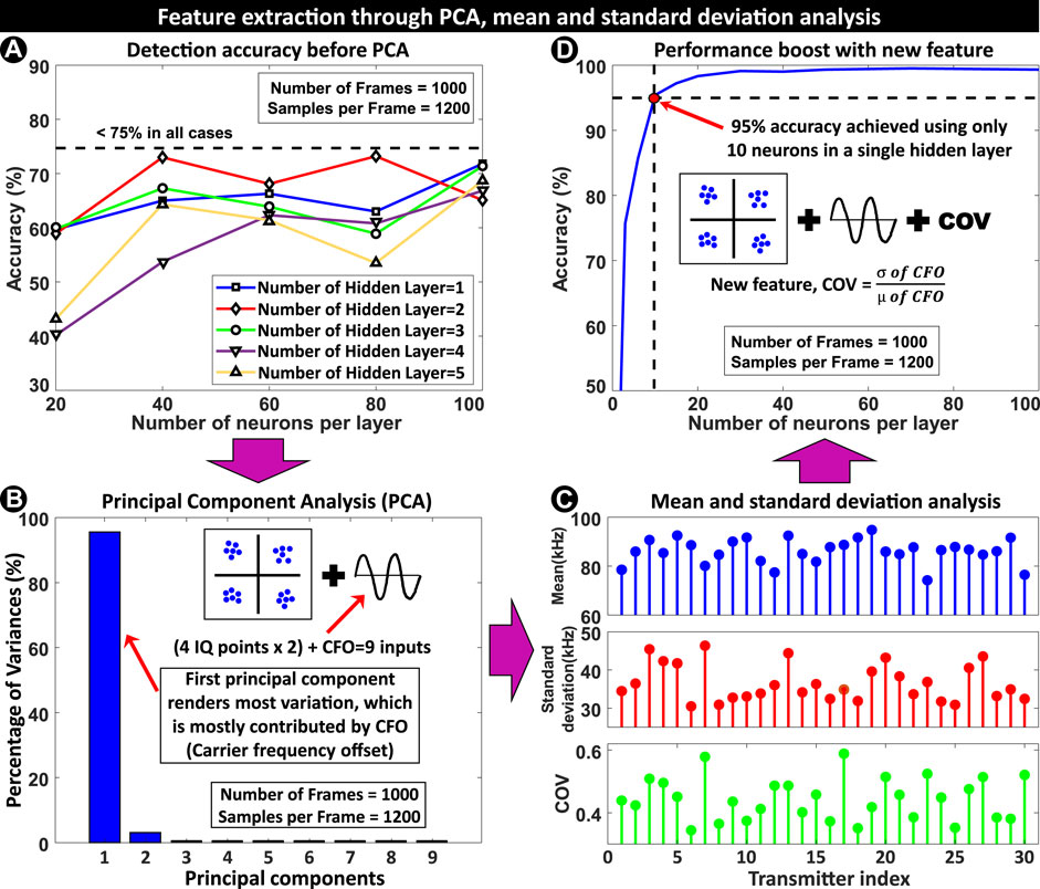
FIGURE 4. (A) Accuracy vs. the number of neurons in each hidden layer. Even after increasing the number of hidden layers, the accuracy remains $<75\%$. (B) Principal Component Analysis (PCA) reveals that the first principal component (PC) causes most variation, which in turn depends mostly on the carrier frequency offset, CFO. (C) Mean (μ) and standard deviation (σ) of the dominant feature (CFO) were analyzed in search of a new feature. It reveals that these statistical parameters vary significantly among transmitters. So, their ratio or coefficient of frequency offset variation, COV = $\frac{\text{standard\hspace{0.17em}deviation}(\sigma )\text{of\hspace{0.17em}CFO}}{\text{mean}(\mu )\text{of\hspace{0.17em}CFO}}$ is taken as the 10^th feature. (D) The inclusion of COV shows significant improvement in the detection accuracy. Using a single hidden layer with only 10 neurons, 95% accuracy is achieved, and $>99.8\%$ accuracy is reached for $>50$ neurons.

4.3 Statistical Analysis

4.3.1 Principal Component Analysis

We start the investigation by performing Principal Component Analysis (PCA) with feature matrix as input (each feature represents one input dimension). Figure 4B shows the principal components and their contribution to the variances. The first principal component (PC) contributes to most of the variances and the input to PC mapping reveals that the CFO is the most dominant feature. So, an in-depth statistical property analysis of the CFO can help in deriving a new feature.

4.3.2 Moment Analysis

Since CFO varies from frame to frame (i.e., with time), it is intuitive to look at the moments of their distribution. Specifically, we want to look at first and second-order moments (mean and variance). Figure 4C shows the absolute values of mean and standard deviation (square root of variance) of CFO. These parameters vary significantly from TX to TX in most cases. And even if for any two TX, the mean is similar, the standard deviation is different, and vice versa. If they can be combined to form a new feature, that can provide significant discrimination among transmitters and lead to much better accuracy. In statistics, the ratio of standard deviation and mean is known as the coefficient of variation. So, using this statistical parameter, we form a new feature named the coefficient of frequency offset variation (COV) which is defined as:

$COV=\left|\frac{\mathit{\text{Standard deviation of CFO}}}{\mathit{\text{Mean of CFO}}}\right|$

4.4 Performance Using Coefficient of Frequency Offset Variation Feature

COV is included as the 10^th feature in our existing feature matrix. From PCA analysis, it is already revealed that the I-Q features contribute to much fewer variances and can be discarded by trading some accuracy. Since our goal is to achieve maximum possible accuracy, we still keep them as features. Also, I-Q values contain channel information, which will help the NN to compensate for the wireless channel (channel effect is explained in subsection 5.5).

After including COV as the 10^th feature, our neural network was trained, validated, and tested again with the new feature matrix. Figure 4D shows that the performance of the network has improved drastically. With just a single hidden layer, $>95\%$ accuracy can be achieved using 10 neurons and can hit up to 99.9% accuracy by increasing the number of neurons.

5 Evaluation of Design Parameters

5.1 Effect of Number of Samples

Figure 5A shows the plot of detection accuracy versus the number of samples in each frame for different neural networks. The general trend (Bold red arrow) is that, for each NN configuration, detection accuracy improves with the increase in the number of samples (along the x-axis). This is expected because a higher number of samples provide more information and hence better performance. We want to mention that there might be some temporary sporadic drops in accuracy (as in the red line where accuracy slightly drops from 50 to 100 samples), but that does not represent the general trend which clearly shows that more samples translate to better accuracy. Also, $>95\%$ accuracy point is reached at around 150 samples per frame which is equivalent to 12.5 ms of total data (or 1.8 ms test data). Hence, we can reach the 95% accuracy bar using quite small test data.

FIGURE 5

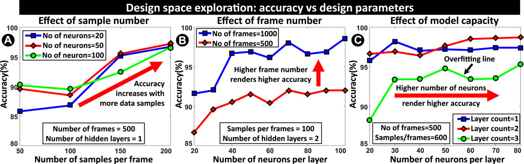
FIGURE 5. (A) Detection accuracy vs. the number of samples per frame for different neural networks which shows a trend of accuracy improvement (indicated by red arrow) with the increase in sample number. (B) Detection accuracy for different frame numbers shows higher frame number renders better performance. (C) Detection accuracy versus the number of neurons per layer. The general trend shows that accuracy improves with the increase in the number of neurons in each layer. Also, accuracy typically improves with more hidden layers until the higher model order causes overfitting and degrades performance.

5.2 Effect of the Number of Frames in Feature Set

Figure 5B shows accuracy versus the number of neurons per layer for two different frame numbers, 500 and 1000. With a higher frame number, the information content of each transmitter device increases. As the NN gets more information about the device, its performance improves and the detection accuracy gets better as shown by the blue (1000 frames) and red lines (500 frames) respectively. We can generalize the previous subsection (sample number effect) and this subsection as this: more data render better performance.

5.3 Effect of the Neural Network Parameters

Figure 5C shows the plots of accuracy versus the number of neurons in each hidden layer. As the number of neurons increases along the x-axis, accuracy, in general, gets better (there might be sporadic peaks or drops as in the case of the blue line with an outlier peak at 30 neurons, but this does not represent a general trend). Also, as the number of hidden layers increases, the network performs better initially (from blue to red line), but later it creates an overfitting problem (the green line) where the model capacity is too large compared to data. This phenomenon directly manifests itself as a degradation in performance. Hence, there is an optimum model capacity up to which accuracy increases, and beyond that accuracy drops.

5.4 Using Simple Machine Learning Algorithm

It has been observed that the COV values vary significantly among different transmitters. When a simple feature displays a significant separation among different classes, it can be modeled with a complex if-else ladder structure. This implies that even simple ML algorithms (e.g. Tree) can show good results. Figure 6A shows that some popular ML algorithm achieves $>95\%$ accuracy.

FIGURE 6

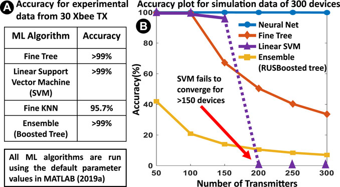
FIGURE 6. (A) Popular ML algorithms show high accuracy for 30 Xbee devices. (B) The accuracy of simple ML networks drops when the number of TX is large, wherein the neural network still holds up with $>99.9\%$ accuracy.

The true power of the neural network comes into play when the number of TX increases as shown in Figure 6B. For this, features are generated for 300 TX devices following a Gaussian distribution (as in (Chatterjee et al., 2019)) with the same mean and variance as that of the original 30 TX devices, for both inter and intra-class variations. Figure 6B shows that as the number of TX increases, accuracy falls after a certain point ($\sim 100$ TX) even for support vector machines (SVM), and it fails to converge for $>150$ TX.

5.5 Effect of Wireless Channel

So far, nonidealities due to TX were considered and the wireless channel was ignored (TX and RX are connected via SMA cable). But the channel itself adds some nonidealities. Here, the effect of a static wireless channel (1 m of fixed TX-RX separation) has been analyzed. Figure 7 shows accuracy versus neuron number in a single layer, with and without the wireless channel. For iso-accuracy of 95%, wireless channel demands slightly higher model capacity (10 vs. 15 neurons). But when the number of neurons increases $(>50)$, both curves merge and render similar accuracy.

FIGURE 7

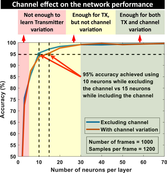
FIGURE 7. Comparison of the network performance in the cases of including and excluding the wireless channel data. The network needs 15 neurons compared to 10 neurons in a hidden layer to achieve 95% accuracy for the case where the channel is considered. But with higher model capacity, both lines converge and the network learns the channel effect on data. d the network learns the channel effect on data. The light red box shows the region where the network fails to learn transmitter variation, light yellow box shows the region where the network learns transmitter variation but fails to learn the variation due to the wireless channel. The light green box shows the region where the network learns both the transmitter and channel variation properly.

In one of our recent works (Bari et al., 2021b), we applied RF-PUF on the ORACLE dataset which contains data for 16 USRP X310 TX for both static and quasi-static (variable TX-RX separation) cases with a channel length varying from 2 to 62 ft. We have shown that RF-PUF achieves 100% accuracy up to 38 ft and $>95\%$ accuracy even at 62 ft channel length. This result confirms that the RF-PUF approach can make the channel compensation with the help of NN and render high performance even in a long wireless channel. On a side note, that work combined with current work, also confirms that RF-PUF achieves high accuracy on experimental data in different platforms (XBee vs. USRP radios using WiFi) for different devices.

5.6 Computational Complexity of RF-PUF

RF-PUF does not add any additional circuitry on the TX side. Hence there is no extra computational burden at the TX end. On the receiver side, it employs just a multilayer perceptron (MLP) or NN along with the standard receiver. The standard receiver corrects the received signal and in the process discards various system-level nonidealities which are used as features to the NN. Hence, the computational complexity of RF-PUF is that of a neural network. For an n-dimensional input (n = 10 for our case), the training phase (done only once) has a computational complexity on the order of $\mathcal{O}(n^5)$, whereas the inference phase has a computational complexity on the order of $\mathcal{O}(n^4)$ (a derivation of the orders can be found at (Fredenslund 2022)). Also, the statistical feature formation requires mean and standard deviation calculation which has computational complexity in the order of $\mathcal{O}(n^2)$, which is negligible compared to the inference order.

6 Analysis of PUF Properties

PUF response to a particular challenge is a probabilistic function. In this section, we will determine intra-PUF hamming distance and inter-PUF hamming distance and discuss various PUF properties ((Maes 2013; Plusquellic 2018)) in light of those distances.

6.1 Constructability

A PUF class $\mathbb{P}$ is constructible if we can create a new PUF instance $pu{f}_m\in \mathbb{P}$ through a process, $\mathbb{P}$.Create: $pu{f}_m\leftarrow \mathbb{P}\text{.Create}$, where puf_m has entropy that makes it distinct from other PUF instances puf_n,n≠m. In the case of RF-PUF, the source of entropy is the manufacturing process variation. During fabrication of ICs, we have within die and die-to-die variation which is due to the limitation of the manufacturing process. In contrast to many other PUF classes where we need a separate mechanism for PUF instance creation, the manufacturing process of the integrated circuit itself serves as the creation process for RF-PUF which is one of its advantages.

6.2 Evaluability

A PUF class $\mathbb{P}$ is evaluable if for a random PUF instance $pu{f}_m\in \mathbb{P}$ and a random challenge (x), we can evaluate a response y: y ← puf_m(x). In our case, the challenge is a randomly generated bitstream in MATLAB that is fed into the transmitter and the corresponding response is the analog signal that contains the unique physical signature of the transmitter.

6.3 Inter PUF Distance - Uniqueness

Uniqueness refers to how different each instance of a PUF class $\mathbb{P}$ is from each other. A measurement metric that is used to represent PUF uniqueness is called inter-PUF hamming distance and is defined as:

$H{D}_{inter}\cong distance\left[Y_m^{\alpha }\left(x\right),Y_n^{\alpha }\left(x\right)\right]$

Here, $Y_m^{\alpha }(x)$ and $Y_n^{\alpha }(x)$ are the responses from puf_m and puf_n (two instances of PUF class $\mathbb{P}$) under the same environmental condition α and same challenge x. Ideally, these inter-chip hamming distances should be much greater than any intra-chip hamming distances to distinguish them separately. In our experiment, our PUF class $\mathbb{P}$ = RF-PUF and puf_i, (where i = 1, 2, …, 30) are the instances of that class (30 Xbee devices).

To calculate HD_inter, the first 1000 frames from each of the transmitters are taken. Each frame contains 3600 samples. Our features remain unchanged: CFO, eight I-Q component values, and COV. But after taking 10 features from each of 1000 frames, instead of using them as a feature matrix for each transmitter, the mean values of the features are taken across all the frames. This means that instead of representing each transmitter as a 10 × 1000 feature matrix, it is represented as a 10 × 1 feature vector. The reason for taking the average value across the frames is that the frames have an associated timestamp with them i.e., each frame data are collected from time to time. So, each frame faces slightly different environmental conditions such as heating of the transmitter due to data transmission for a long time, external interference, noise, etc. Averaging the feature values across a large number of frames mitigates the environmental factors, especially noise. Also, taking the first 1000 frames from each transmitter ensures the same initial heating pattern across devices. So the final outcome is that the feature vector for each transmitter has a very similar environmental factor α, which is one of the conditions of inter-chip hamming distance calculation.

After taking the feature vector from each transmitter, the Euclidean distance was calculated in ten-dimensional feature space as hamming distance. For puf_m, let us denote CFO_m = carrier frequency offset, COV_m = coefficient of frequency offset variation, I_k,m = in-phase component in the k^th quadrant, and Q_k,m = quadrature-phase component in the k^th quadrant. Then distance d_m,n between puf_m and puf_n instances is given by:

$\begin{array}{cc}\hfill d_{m,n}^2=& {\left(CF{O}_m-CF{O}_n\right)}^2+{\left(CO{V}_m-CO{V}_n\right)}^2+\hfill \\ \hfill & \sum _{k=1}^4{\left(I_{k,m}-I_{k,n}\right)}^2+\sum _{k=1}^4{\left(Q_{k,m}-Q_{k,n}\right)}^2\hfill \end{array}(1)$

The inter-chip distances were calculated for each transmitter with respect to all 30 transmitters (including the chip under test), which leads to a 30 × 30 symmetric matrix (upper and lower triangular matrices with same values since d_m,n = d_n,m = inter-chip distance between puf_m and puf_n) with a principal diagonal of zeros (self-distance). It is found that the worst-case scenario with minimum distance, HD_inter,min = 0.2307, and the best-case scenario with maximum distance, HD_inter,max = 10.149.

In literature, often a mean inter-puf distance, μ_inter, is reported which is the average of all HD_inter. The formula is:

$\begin{array}{cc}\hfill {\mu }_{inter}& =\overline{H{D}_{inter}}\hfill \\ \hfill & =\frac{2}{N_{puf}\times \left(N_{puf}-1\right)\times N_{chal}}\sum H{D}_{inter}\hfill \end{array}$

Where N_puf is the number of puf instances (N_puf = 30 for us), and N_chal is the number of challenges (N_chal = 1, since we are not varying our challenge). Using this formula, we find that μ_inter = 3.703.

Figure 8C shows the probability mass function distribution of $435(=\frac{30\times 29}{2})$ inter-PUF distances. The density function is right-skewed, that’s why Weibull fitting (which is exponential in nature) fits it more accurately than normal distribution fitting. This fitting shows that on the right side the curve is more sparse but on the left side it is more centered instead of being sparse, which is good because that will ensure that the inter-PUF values don’t go to overlap intra-PUF distances which should ideally be at zero.

FIGURE 8

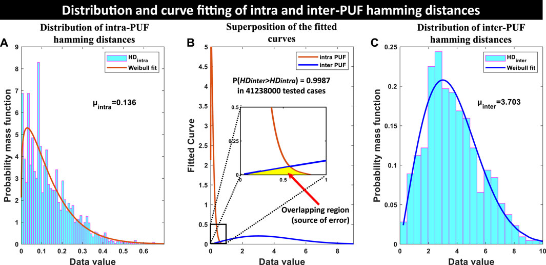
FIGURE 8. Data distribution of (A) intra-PUF hamming distances and (C) inter-PUF hamming distances. Due to skewness, Weibull distribution fitting is a more accurate representation in these cases. (B) The two Weibull curves are superimposed on top of each other. It is seen that there is a very slight overlap (yellow region) between the curves which is shown in a zoomed inset. Although trivial, this overlapping is the source of the detection error.

6.4 Intra PUF Distance–Reliability

PUF responses are in general dependent on various environmental factors that render any PUF instance response as a probabilistic function. This means that a particular PUF instance can provide slightly different values of features based on varying environmental conditions. For authentication purposes, this poses an issue. Reliability refers to how resilient a PUF instance is against environmental factors e.g. noise, interference, temperature, supply voltage, etc.

A measurement metric that is used to represent how reliable a particular instance of a PUF class $\mathbb{P}$ is intra-puf hamming distance and is defined as:

$H{D}_{intra}\cong distance\left[Y_m^{\alpha }\left(x\right),Y_m^{\beta }\left(x\right)\right]$

Here, $Y_m^{\alpha }(x)$ and $Y_m^{\beta }(x)$ are the responses from puf_m under two distinct environmental conditions α and β and same challenge x. Many HD_intra distances are calculated at different environmental conditions. Ideally, these intra-chip hamming distances should be zero.

To calculate HD_intra, we follow two steps. Let us consider one particular PUF instance puf_m. In step 1, the first 1000 frames (frame number 1 to frame number 1000) were taken from puf_m, each frame containing 3600 samples. Then mean values of the previously mentioned ten features were taken just as before to represent it as a 10 × 1 feature vector. Let us represent this vector as f_v,1. Then in step 2, the first 5 frames are skipped and the next 1000 frames are taken from frame number = 6 to frame number = 1005. Step 1 is repeated here to get the next feature vector f_v,2. Then next 1000 frames are taken from frame number = 11 to frame number = 1010 and a feature vector f_v,3 is formed. This process is repeated 80 times to form 80 different feature vectors f_v,α; α = 1, 2, … , 80. These 10 × 1 feature vectors are stacked together to form a feature vector set f_set,m of size 10 × 80 for puf_m. The whole process is then repeated for all 30 devices.

The purpose of taking frame-shifted or time-shifted frame groups is to consider the time factor. Each frame has a duration of 0.6 ms, so 5 frames gap in between two frame groups renders a time difference of at least 3 ms (in reality the difference is much larger since the transmitter transmits data for a small time and most of the frames are just noise which are filtered in data pre-processing step). The 80 time-spaced frames, in reality, cover almost half a minute. Our 2.4 GHz clock will have LO drift cycle time in the nanoseconds range. Hence, half-minute data can incorporate significant environmental factors into frame data. So, it can be assumed that the feature vectors f_v,α; α = 1, 2, … , 80 in feature vector set f_set,m of puf_m represents α = 80 different environmental conditions.

Now, for each instance puf_m, Euclidean distance is calculated in 10-dimensional feature space among the feature vectors in the feature vector set using Eq. 1. This results in a symmetric matrix of size 80 × 80 with a principal diagonal of zeros. This process is repeated for other transmitters as well. Essentially it gives us 30 matrices of size 80 × 80 for intra-PUF distances. In the best-case scenario, the minimum distance is HD_intra,min = 7.23 × 10^–5 and in the worst case scenario, the maximum distance is HD_intra,max = 0.73.

Figure 8A shows the probability mass function distribution of $94800(=\frac{30\times 80\times 79}{2})$ intra-PUF distances. The density function is right-skewed and Weibull distribution gives better fitting for it just like inter-PUF cases. This fitting shows that on the left side the curve is strongly centered towards zero, but has a diminishing trail on the right. this trail goes on to overlap inter-puf distances slightly and causes a few detection errors. Detection probability is discussed in the next subsection.

Finally, a mean intra-PUF distance, μ_intra, is calculated which is the average of all HD_intra. The formula is:

$\begin{array}{cc}\hfill {\mu }_{intra}& =\overline{H{D}_{intra}}\hfill \\ \hfill & =\frac{2}{N_{puf}\times N_{chal}\times \alpha \times \left(\alpha -1\right)}\sum H{D}_{intra}\hfill \end{array}$

Where N_puf is the number of puf instances (N_puf = 30 for us), N_chal is the number of challenges (N_chal = 1, since we are not varying our challenge) and α is the number of environmental conditions (α = 80 in our study). Using this formula, it is found that μ_intra = 0.136.

6.5 Identifiability

In the previous two subsections, both inter-PUF and intra-PUF hamming distances and their mean values: μ_inter = 3.703 and μ_intra = 0.136 are calculated. Their comparison shows that μ_inter > μ_intra, which establishes that on average the PUF instances can be distinguished from each other. But the mean value does not depict the full story. Figure 8B shows the fitted distribution curves superimposed on each other. The brown curve (intra-PUF distribution) is skewed to the left and the blue curve (inter-PUF distribution) is skewed to the right and they mostly cover different regions. However, there is slight overlapping between them which is shown in the inset as a zoomed version of the overlapping area. Ideally, there should be no overlapping. But in a practical scenario, this overlapping region is the source of detection error.

From the definition of identifiability, a PUF class $\mathbb{P}$ is identifiable if it is reliable as well as unique, and if the probability of inter-PUF variation being greater than intra-PUF variation is very high. Mathematically:

$Probability\left(H{D}_{inter}>H{D}_{intra}\right)\approx 1$

In the previous two subsections, $94800(=\frac{30\times 80\times 79}{2})$ intra-PUF distances and $435\left(=\frac{30\times 29}{2}\right.$ inter-PUF distances have been calculated. Now, each of these inter-puf distances is compared with each of the intra-PUF distances that leads us to 435 × 94800 = 41238000 cases, among which, HD_inter > HD_intra is found in 41184206 cases.

$\mathit{P}\mathit{r}\mathit{o}\mathit{b}\mathit{a}\mathit{b}\mathit{i}\mathit{l}\mathit{i}\mathit{t}\mathit{y}\left(\mathit{H}{\mathit{D}}_{\mathit{i}\mathit{n}\mathit{t}\mathit{e}\mathit{r}}>\mathit{H}{\mathit{D}}_{\mathit{i}\mathit{n}\mathit{t}\mathit{r}\mathit{a}}\right)=\mathbf{0.9987}$

This is a very high probability and close to 1. This proves that RF-PUF has strong identifiability and this property along with reliability, uniqueness, constructability, and evaluability manifests RF-PUF as a distinct PUF class. This is the first-ever experimental validation of RF-PUF as a distinct and strong PUF class by itself.

7 Possible Attack Models on RF-PUF

RF-PUF does not store any digital key and hence, is not susceptible to malicious PUF models which assume that the adversary can have access to all the challenge-response pairs through a built-in logger software/implanted Trojan. However, there is a possibility of a machine learning-based attack that needs to be discussed (Figure 10). For RF-PUF, ML attack is a two-step process:

• Step 1: model/profile the victim TX (Unsupervised)

• Step 2: use that model for spoofing/replay attacks

In step 1, the rogue device tries to learn the feature/parameter values of the victim TX. Unlike the intended RX, this is an unsupervised problem for the attacker. We have utilized k-means clustering to divide the feature map into 30 clusters and compare the predicted and true labels (Figure 9). The process was repeated 1,000 times as k-means isn’t unique without specific conditions. Our analysis shows that clustering achieves $\sim 3.63\%$ accuracy on average, which is very close to the probability of random detection $(\frac{1}{30}=3.3\%)$. So, practically it is almost impossible to get the right feature value and label.

FIGURE 9

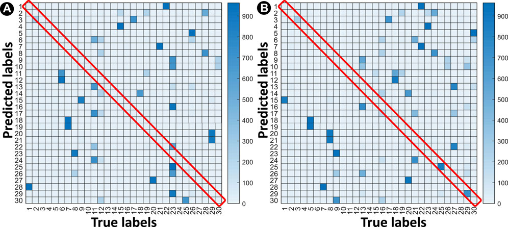
FIGURE 9. Heatmap of unsupervised learning in the attacker using k-means clustering. (A) The worst-case accuracy of 0.09% and (B) the best-case accuracy of 6.8%. Repeated clustering 1000 times shows 3.63% accuracy on average.

If somehow the attacker succeeds in step 1, then in step 2, the attacker needs to produce an RF signal that contains the same imperfections as the victim TX with high accuracy. This requires a high speed and high-resolution circuitry. Figure 10 shows that the physical signature of the transmitter, S, goes through transformation T_TX at TX and T_RX at RX. The transformations in the attacker are T_A, T_ML1, T_ML2, and T_D respectively. Full transformation for the original device is T_RX (T_TX(S)) and for the adversary is T_RX (T_D (T_ML2 (T_ML1 (T_A (T_TX(S)))))). The adversary ML2 framework needs to make these two transformations equal by undoing the effect of its ADC/DAC which requires almost infinite resolution, rendering it practically impossible (typical ADC/DAC are 8/16-bit). This Resolution limitation in ADC/DAC and bandwidth limitation in filters and other RF components also prevent replay attack, which requires the attacker to convert the TX signal in the digital domain, incorporate malicious contents and then transform it back into the RF domain with very high precision. Further analysis of precision requirements for a practical attack will be included in future work. The robustness of RF-PUF against malicious PUF model, ML attack, and replay attack proves its strong candidacy of employment for RF security.

FIGURE 10

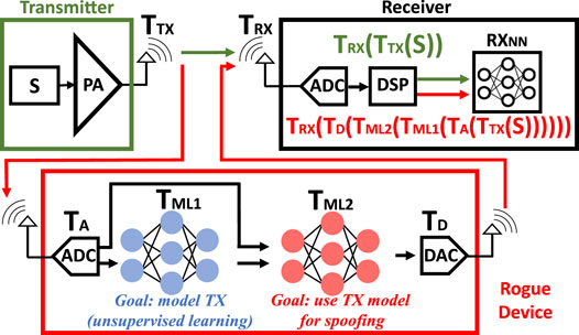
FIGURE 10. ML attack model. Adversary ML networks cannot undo the effect of ADC and DAC which requires extremely high precision and resolution, making the attack impractical.

8 Conclusion

In this work, data collected from off-the-shelf commodity components (30 Xbee modules) were used to develop a new feature called the coefficient of frequency offset variation (COV) through PCA and moment analysis. The new feature leads to 95% accuracy for a single hidden layer with 10 neurons and $>99.8\%$ accuracy for a single hidden layer with $>50$ neurons, for the first time in literature without any assisting digital preamble. The dataset containing 155.4 GB of data has also been released for public use. The design space has been explored and the effect of the wireless channel is analyzed to provide design insights. The scalability issue of simple ML algorithms for high accuracy has also been explored. The PUF properties of RF-PUF have been explored in detail. The inter-PUF and intra-PUF hamming distances are calculated and with their distribution, it has been shown that they have trivial overlapping. A detailed analysis reveals that the probability of HD_inter > HD_intra = 0.9987, which resonates with the claim that RF-PUF has a very high device authentication probability. Finally, possible important attack models are discussed and the robustness of RF-PUF against them is analyzed. This work experimentally validates RF-PUF with high accuracy, which can contribute to a secure authentication system using inherent physical signatures without extra power, area, or computational overhead on the resource-constrained IoT transmitter side.

Data Availability Statement

The datasets presented in this study can be found in online repositories. The names of the repository/repositories and accession number(s) can be found below: https://github.com/SparcLab/Sparclab-RF-PUF-Dataset.

Author Contributions

PA prepared an initial framework of 4 Xbee devices for data collection. MB has set up the test environment, prepared and conducted the experiment with 30 Xbee modules in a renewed framework, processed data, performed the statistical analysis, feature engineering, and evaluated performance. BC helped both PA and MB in setting up the experimental framework and data processing as well as guiding with technical feedback. SS supervised the whole work. MB wrote the manuscript while both BC and SS helped in writing the paper, reviewing and updating it as needed.

Funding

This work was supported in part by the National Science Foundation, under Grant 1935573.

Conflict of Interest

The authors declare that the research was conducted in the absence of any commercial or financial relationships that could be construed as a potential conflict of interest.

Publisher’s Note

All claims expressed in this article are solely those of the authors and do not necessarily represent those of their affiliated organizations, or those of the publisher, the editors and the reviewers. Any product that may be evaluated in this article, or claim that may be made by its manufacturer, is not guaranteed or endorsed by the publisher.

References

Albawi, S., Mohammed, T. A., and Al-Zawi, S. “Understanding of a Convolutional Neural Network,” in 2017 international conference on engineering and technology (ICET) (IEEE), 1–6. doi:10.1109/icengtechnol.2017.8308186

CrossRef Full Text | Google Scholar

Alotaibi, B., and Elleithy, K. (2016). A New Mac Address Spoofing Detection Technique Based on Random Forests. Sensors 16 (3), 281. doi:10.3390/s16030281

PubMed Abstract | CrossRef Full Text | Google Scholar

Bari, M. F., and Anowarul Fattah, S. (2020). Epileptic Seizure Detection in EEG Signals Using Normalized IMFs in CEEMDAN Domain and Quadratic Discriminant Classifier. Biomed. Signal Process. Control. 58, 101833. doi:10.1016/j.bspc.2019.101833

CrossRef Full Text | Google Scholar

Bari, M. F., Chatterjee, B., and Sen, S. (2021a). “DIRAC: Dynamic-IRregulAr Clustering Algorithm with Incremental Learning for RF-Based Trust Augmentation in IoT Device Authentication,” in 2021 IEEE International Symposium on Circuits and Systems (ISCAS) (IEEE), 1–5.

CrossRef Full Text | Google Scholar

Bari, M. F., Chatterjee, B., Sivanesan, K., Yang, L. L., and Sen, S. (2021b). “High Accuracy RF-PUF for EM Security through Physical Feature Assistance Using Public Wi-Fi Dataset,” in 2021 IEEE MTT-S International Microwave Symposium (IMS), 108–111. doi:10.1109/ims19712.2021.9574917

CrossRef Full Text | Google Scholar

Bari, M. F., and Sen, S. (2022). Sparclab RF-PUF Dataset,” GitHub. [Online]. Available at: https://github.com/SparcLab/Sparclab-RF-PUF-Dataset (Accessed March 6, 2022).

Google Scholar

Barth, A., Jackson, C., and Mitchell, J. C. (2008). “Robust Defenses for Cross-Site Request Forgery,” in Proceedings of the 15th ACM conference on Computer and communications security, 75–88. doi:10.1145/1455770.1455782

CrossRef Full Text | Google Scholar

Bertoncini, C., Rudd, K., Nousain, B., and Hinders, M. (2012). Wavelet Fingerprinting of Radio-Frequency Identification (Rfid) Tags. IEEE Trans. Ind. Electron. 59 (12), 4843–4850. doi:10.1109/tie.2011.2179276

CrossRef Full Text | Google Scholar

Bihl, T. J., Bauer, K. W., and Temple, M. A. (2016). Feature Selection for RF Fingerprinting with Multiple Discriminant Analysis and Using ZigBee Device Emissions. IEEE Trans. Inf. Forensics Secur. 11 (8), 1862–1874. doi:10.1109/TIFS.2016.2561902

CrossRef Full Text | Google Scholar

Brik, V., Banerjee, S., Gruteser, M., and Oh, S. (2008). “Wireless Device Identification with Radiometric Signatures,” in Proceedings of the 14th ACM International Conference on Mobile Computing and Networking (MobiCom ’08) (New York, NY, USA: Association for Computing Machinery), 116–127. doi:10.1145/1409944.1409959

CrossRef Full Text | Google Scholar

Chacko, J. (2017). “Physical Gate Based Preamble Obfuscation for Securing Wireless Communication,” in International Conference on Computing, Networking and Communications (ICNC), 293–297.

CrossRef Full Text | Google Scholar

Chatterjee, B., Das, D., Maity, S., and Sen, S. (2019). RF-PUF: Enhancing IoT Security through Authentication of Wireless Nodes Using In-Situ Machine Learning. IEEE Internet Things J. 6 (1), 388–398. doi:10.1109/JIOT.2018.2849324

CrossRef Full Text | Google Scholar

Chomsiri, T. (2007). “HTTPS Hacking protection,” in 21st International Conference on Advanced Information Networking and Applications Workshops (AINAW’07), 590–594.1

CrossRef Full Text | Google Scholar

Creswell, A., White, T., Dumoulin, V., Arulkumaran, K., Sengupta, B., and Bharath, A. A. (2018). Generative Adversarial Networks: An Overview. IEEE Signal. Process. Mag. 35 (1), 53–65. doi:10.1109/msp.2017.2765202

CrossRef Full Text | Google Scholar

Danev, B., and Capkun, S. (2009). “Transient-based Identification of Wireless Sensor Nodes,” in 2009 International Conference on Information Processing in Sensor Networks, 25–36.

Google Scholar

Danev, B., Heydt-Benjamin, T. S., and Capkun, S. (2009). “Physical-layer Identification of Rfid Devices,” in USENIX Security Symposium, 199–214.

Google Scholar

Ding, L., Wang, S., Wang, F., and Zhang, W. (2018). Specific Emitter Identification via Convolutional Neural Networks. IEEE Commun. Lett. 22 (12), 2591–2594. doi:10.1109/lcomm.2018.2871465

CrossRef Full Text | Google Scholar

Fredenslund, K. (2022). Computational Complexity of Neural Networks. [Online]. Available at: https://kasperfred.com/series/introduction-to-neural-networks/computational-complexity-of-neural-networks (Accessed March 6, 2022).

Google Scholar

Guo, X., Zhang, Z., and Chang, J. (2019). “Survey of mobile Device Authentication Methods Based on Rf Fingerprint,” in IEEE INFOCOM 2019 - IEEE Conference on Computer Communications Workshops (Infocom Wkshps), 1–6. doi:10.1109/infocomwkshps47286.2019.9093755

CrossRef Full Text | Google Scholar

Hall, J., Barbeau, M., and Kranakis, E. (2003). Detection of Transient in Radio Frequency Fingerprinting Using Signal Phase. Wireless Opt. Commun., 13–18.

Google Scholar

Hanna, S. S., and Cabric, D. (2019). “Deep Learning Based Transmitter Identification Using Power Amplifier Nonlinearity,” in 2019 International Conference on Computing, Networking and Communications (HonoluluHI, USA: ICNC), 674–680. doi:10.1109/ICCNC.2019.8685569

CrossRef Full Text | Google Scholar

Hospodar, G., Gierlichs, B., Mulder, E. D., Verbauwhede, I., and Vandewalle, J. (2011). Machine Learning in Side-Channel Analysis: a First Study. J. Cryptographic Eng. 1 (4), 293. doi:10.1007/s13389-011-0023-x

CrossRef Full Text | Google Scholar

Huang, N. E. (2014). Hilbert-huang Transform and its Applications, 16. New Jersey: World Scientific.

Google Scholar

Huang, Y., and Zheng, H. (2012). “Radio Frequency Fingerprinting Based on the Constellation Errors,” in 2012 18th Asia-Pacific Conference on Communications (APCC), 900–905. doi:10.1109/apcc.2012.6388238

CrossRef Full Text | Google Scholar

Jian, T., Rendon, B. C., Ojuba, E., Soltani, N., Wang, Z., Sankhe, K., et al. (2020). Deep Learning for Rf Fingerprinting: A Massive Experimental Study. IEEE Internet Things M. 3 (1), 50–57. doi:10.1109/iotm.0001.1900065

CrossRef Full Text | Google Scholar

Jagannath, A., Jagannath, J., and Kumar, P. S. P. V. (2022). A Comprehensive Survey on Radio Frequency (RF) Fingerprinting: Traditional Approaches, Deep Learning, and Open Challenges. arXiv [Preprint]. doi:10.48550/arXiv.2201.00680

CrossRef Full Text | Google Scholar

Kennedy, I. O., Scanlon, P., Mullany, F. J., Buddhikot, M. M., Nolan, K. E., and Rondeau, T. W. (2008). “Radio Transmitter Fingerprinting: A Steady State Frequency Domain Approach,” in 2008 IEEE 68th Vehicular Technology Conference, 1–5.

CrossRef Full Text | Google Scholar

Kim, P. (2017). “Convolutional Neural Network,” in MATLAB Deep Learning: With Machine Learning, Neural Networks and Artificial Intelligence (Berkeley, CA: Apress), 121–147. doi:10.1007/978-1-4842-2845-6_6

CrossRef Full Text | Google Scholar

Klein, R. W., Temple, M. A., and Mendenhall, M. J. (2009). Application of Wavelet-Based Rf Fingerprinting to Enhance Wireless Network Security. J. Commun. Netw. 11 (6), 544–555. doi:10.1109/jcn.2009.6388408

CrossRef Full Text | Google Scholar

Kocher, P., Jaffe, J., and Jun, B. (1999). “Differential Power Analysis,” in Annual International Cryptology Conference (Berlin, Heidelberg: Springer), 388–397. doi:10.1007/3-540-48405-1_25

CrossRef Full Text | Google Scholar

Kumar, K., Kaur, P., and Amritsar, G. N. D. U. (2015). “Vulnerability Detection of International mobile Equipment Identity Number of Smartphone and Automated Reporting of Changed IMEI Number,” in International Journal of Computer Science and Mobile Computing, 527–533.45

Google Scholar

Liu, P., Qiu, X., and Huang, X. (2016). Recurrent Neural Network for Text Classification with Multi-Task Learning. arXiv [Preprint]. doi:10.48550/arXiv.1605.05101

CrossRef Full Text | Google Scholar

Lukacs, M., Collins, P., and Temple, M. (2015). Classification Performance Using 'RF‐DNA' Fingerprinting of Ultra‐wideband Noise Waveforms. Electron. Lett. 51 (10), 787–789. doi:10.1049/el.2015.0051

CrossRef Full Text | Google Scholar

Maes, R. (2013). Physically Unclonable Functions: Constructions, Properties and Applications. New York: Springer Science & Business Media. doi:10.1007/978-3-642-41395-7

CrossRef Full Text | Google Scholar

Mao, X., Li, Q., Xie, H., Lau, R. Y., Wang, Z., and Paul Smolley, S. (2017). “Least Squares Generative Adversarial Networks,” in Proceedings of the IEEE international conference on computer vision, 2794–2802. doi:10.1109/iccv.2017.304

CrossRef Full Text | Google Scholar

Medsker, L. R., and Jain, L. C. (2001). Recurrent Neural Networks. Des. Appl. 5, 64–67.

Google Scholar

Nguyen, N. T., Zheng, G., Han, Z., and Zheng, R. (2011). “Device Fingerprinting to Enhance Wireless Security Using Nonparametric Bayesian Method,” in 2011 Proceedings IEEE INFOCOM, 1404–1412. doi:10.1109/infcom.2011.5934926

CrossRef Full Text | Google Scholar

OAuth 2.0, OAuth (2022). [Online] Available at: https://oauth.net/2/(Accessed 14Jan, 2022).

Ometov, A., Bezzateev, S., Mäkitalo, N., Andreev, S., Mikkonen, T., and Koucheryavy, Y. (2018). Multi-factor Authentication: A Survey. Cryptography 21 (1), 1. doi:10.3390/cryptography2010001

CrossRef Full Text | Google Scholar

ORBIT (2022). Open-access Research Testbed for Next-Generation Wireless Networks (Orbit). Available at: https://www.orbit-lab.org/.

Google Scholar

O’Shea, T., and Hoydis, J. (2017). An Introduction to Deep Learning for the Physical Layer. IEEE Trans. Cogn. Commun. Netw. 3 (4), 563–575. doi:10.1109/TCCN.2017.2758370

CrossRef Full Text | Google Scholar

Pal, M. (2005). Random forest Classifier for Remote Sensing Classification. Int. J. remote sensing 26 (1), 217–222. doi:10.1080/01431160412331269698

CrossRef Full Text | Google Scholar

Patel, H. (2015). “Non-parametric Feature Generation for Rf-Fingerprinting on Zigbee Devices,” in 2015 IEEE Symposium on Computational Intelligence for Security and Defense Applications (CISDA), 1–5. doi:10.1109/cisda.2015.7208645

CrossRef Full Text | Google Scholar

Peng, L., Hu, A., Zhang, J., Jiang, Y., Yu, J., and Yan, Y. (2018). Design of a Hybrid RF Fingerprint Extraction and Device Classification Scheme. IEEE Internet Things J. 6 (1), 349–360. doi:10.1109/JIOT.2018.2838071

CrossRef Full Text | Google Scholar

Peng, L., Zhang, J., Liu, M., and Hu, A. (2020). Deep Learning Based Rf Fingerprint Identification Using Differential Constellation Trace Figure. IEEE Trans. Veh. Technol. 69 (1), 1091–1095. doi:10.1109/tvt.2019.2950670

CrossRef Full Text | Google Scholar

Plusquellic, J. (2018). Physical Unclonable Functions 1. [Online]. Available at: http://ece-research.unm.edu/jimp/HOST/slides/PUF1.pdf (Accessed = Feb 6, 2022).

Google Scholar

Quisquater, J.-J., and Samyde, D. (2001). “Electromagnetic Analysis (Ema): Measures and Counter-measures for Smart Cards,” in International Conference on Research in Smart Cards (Berlin, Heidelberg: Springer), 200–210. doi:10.1007/3-540-45418-7_17

CrossRef Full Text | Google Scholar

Rasmussen, K. B., and Capkun, S. (2007). “Implications of Radio Fingerprinting on the Security of Sensor Networks,” in 2007 Third International Conference on Security and Privacy in Communications Networks and the Workshops-Secure Comm 2007 (IEEE, Sep.), 331–340. doi:10.1109/seccom.2007.4550352

CrossRef Full Text | Google Scholar

Robinson, J., Kuzdeba, S., Stankowicz, J., and Carmack, J. M. (2020). “Dilated Causal Convolutional Model for Rf Fingerprinting,” in roc. of 10th Annual Computing and Communication Workshop and Conference (CCWC), 0157. doi:10.1109/ccwc47524.2020.9031257P

CrossRef Full Text | Google Scholar

Roy, D., Mukherjee, T., Chatterjee, M., and Pasiliao, E. (2019). “Detection of Rogue Rf Transmitters Using Generative Adversarial Nets,” in 2019 IEEE Wireless Communications and Networking Conference (WCNC), 1–7. doi:10.1109/wcnc.2019.8885548

CrossRef Full Text | Google Scholar

Sankhe, K., Belgiovine, M., Zhou, F., Angioloni, L., Restuccia, F., D'Oro, S., et al. (2020). No Radio Left behind: Radio Fingerprinting through Deep Learning of Physical-Layer Hardware Impairments. IEEE Trans. Cogn. Commun. Netw. 6 (1), 165–178. doi:10.1109/TCCN.2019.2949308

CrossRef Full Text | Google Scholar

Scanlon, P., Kennedy, I. O., and Liu, Y. (2010). Feature Extraction Approaches to RF Fingerprinting for Device Identification in Femtocells. Bell Labs Tech. J. 15 (3), 141–151. doi:10.1002/bltj.20462

CrossRef Full Text | Google Scholar

Shaw, D., and Kinsner, W. (1997). “Multifractal Modelling of Radio Transmitter Transients for Classification,” in IEEE WESCANEX 97 Communications, Power and Computing. Conference Proceedings, 306–312.

Google Scholar

Siddiqui, M. S., and Verma, D. (2011). “Cross Site Request Forgery: A Common Web Application Weakness,” in 2011 IEEE 3rd International Conference on Communication Software and Networks (IEEE), 538–543. doi:10.1109/iccsn.2011.6014783

CrossRef Full Text | Google Scholar

Soltani, N., Reus-Muns, G., Salehi, B., Dy, J., Ioannidis, S., and Chowdhury, K. (2020). Rf Fingerprinting Unmanned Aerial Vehicles with Nonstandard Transmitter Waveforms. IEEE Trans. Vehicular Technology 69 (12), 15 518–615 531. doi:10.1109/tvt.2020.3042128

CrossRef Full Text | Google Scholar

Symanovich, S. (2019). The Future of IOT: 10 Predictions about the Internet of Things. Norton, 14. [Online]. Available at: https://us.norton.com/internetsecurity-iot-5-predictions-for-the-future-of-iot.html (Accessed Jan, 2022).

Google Scholar

Ting, D. M., Hussain, O., and LaRoche, G. (2015). Systems and Methods for Multi-Factor Authentication. Washington, DC: U.S. Patent and Trademark Office. U.S. Patent No. 9,118,656.

Google Scholar

Ur Rehman, S., Sowerby, K., and Coghill, C. (2012). “Rf Fingerprint Extraction from the Energy Envelope of an Instantaneous Transient Signal,” in 2012 Australian Communications Theory Workshop (CTW), 90–95. doi:10.1109/ausctw.2012.6164912

CrossRef Full Text | Google Scholar

Vo-Huu, T. D., Vo-Huu, T. D., and Noubir, G. (2016). “Fingerprinting Wi-Fi Devices Using Software Defined Radios,” in Proceedings of the 9th ACM Conference on Security & Privacy in Wireless and Mobile Networks, 3–14. doi:10.1145/2939918.2939936

CrossRef Full Text | Google Scholar

Wang, T., Wen, C.-K., Wang, H., Gao, F., Jiang, T., and Jin, S. (2017). Deep Learning for Wireless Physical Layer: Opportunities and Challenges. China Commun. 14 (11), 92–111. doi:10.1109/cc.2017.8233654

CrossRef Full Text | Google Scholar

Wang, X., Wang, X., and Mao, S. (2018). RF Sensing in the Internet of Things: A General Deep Learning Framework. IEEE Commun. Mag. 56 (9), 62–67. doi:10.1109/mcom.2018.1701277

CrossRef Full Text | Google Scholar

Wang, Y., and Yang, J. (2017). “Ethical Hacking and Network Defense: Choose Your Best Network Vulnerability Scanning Tool,” in 2017 31st International Conference on Advanced Information Networking and Applications Workshops (WAINA), 110–113. doi:10.1109/waina.2017.39

CrossRef Full Text | Google Scholar

Xie, F., Wen, H., Li, Y., Chen, S., Hu, L., Chen, Y., et al. (2018). Optimized Coherent Integration-Based Radio Frequency Fingerprinting in Internet of Things. IEEE Internet Things J. 5 (5), 3967–3977. doi:10.1109/jiot.2018.2871873

CrossRef Full Text | Google Scholar

Xu, Q., Zheng, R., Saad, W., and Han, Z. (2016a). Device Fingerprinting in Wireless Networks: Challenges and Opportunities. IEEE Commun. Surv. Tutorials. 18, 94–104. doi:10.1109/COMST.2015.2476338

CrossRef Full Text | Google Scholar

Xu, Q., Zheng, R., Saad, W., and Han, Z. (2016b). Device Fingerprinting in Wireless Networks: Challenges and Opportunities. IEEE Commun. Surv. Tutorials 18 (1), 94–104. doi:10.1109/comst.2015.2476338

CrossRef Full Text | Google Scholar

Yuan, Y., Huang, Z., Wu, H., and Wang, X. (2014). Specific Emitter Identification Based on Hilbert-Huang Transform‐based Time-Frequency-Energy Distribution Features. IET Commun. 8 (13), 2404–2412. doi:10.1049/iet-com.2013.0865

CrossRef Full Text | Google Scholar

Zhang, C., Patras, P., and Haddadi, H. (2019). Deep Learning in mobile and Wireless Networking: A Survey. IEEE Commun. Surv. Tutorials 21 (3), 2224–2287. doi:10.1109/comst.2019.2904897

CrossRef Full Text | Google Scholar

Zhao, C., Chen, C., Cai, Z., Shi, M., Du, X., and Guizani, M. (2018). “Classification of Small Uavs Based on Auxiliary Classifier Wasserstein gans,” in 2018 IEEE Global Communications Conference (GLOBECOM), 206–212. doi:10.1109/glocom.2018.8647973

CrossRef Full Text | Google Scholar

Zhuo, F., Huang, Y., and chen, J. (2017). Radio Frequency Fingerprint Extraction of Radio Emitter Based on I/q Imbalance. Proced. Computer Sci. 107, 472–477. doi:10.1016/j.procs.2017.03.092

CrossRef Full Text | Google Scholar

Zong, L., Xu, C., and Yuan, H. (2020). “A Rf Fingerprint Recognition Method Based on Deeply Convolutional Neural Network,” in Proc. of IEEE 5th Information Technology and Mechatronics Engineering Conference (ITOEC), 1778–1781. doi:10.1109/itoec49072.2020.9141877

CrossRef Full Text | Google Scholar