 Daniele Santi1,2*†
 Giorgia Spaggiari2
 Antonio R. M. Granata2
 Monica Setti3
 Simonetta Tagliavini4Tommaso Trenti4
 Manuela Simoni1,2
- 1Unit of Endocrinology, Department of Biomedical, Metabolic and Neural Sciences, University of Modena and Reggio Emilia, Modena, Italy
- 2Unit of Endocrinology, Department of Medical Specialties, Azienda Ospedaliero-Universitaria of Modena, Ospedale Civile of Baggiovara, Modena, Italy
- 3Service of Clinical Engineering, Azienda Ospedaliero-Universitaria of Modena, Modena, Italy
- 4Department of Laboratory Medicine and Anatomy Pathology, Azienda USL of Modena, Modena, Italy
Environmental rhythmicity is able to affect the hypothalamic-pituitary-gonadal axis in several animals to achieve reproductive advantages. However, conflicting results were obtained when assessing the environmental-dependent rhythmicity on reproductive hormone secretion in humans. This study was designed to evaluate seasonal fluctuations of the main hormones involved in the hypothalamic-pituitary-gonadal axis in men, using a big data approach. An observational, retrospective, big data trial was carried out, including all testosterone, luteinizing hormone (LH) and follicle-stimulating hormone (FSH) measurements performed in a single laboratory between January 2010 and January 2019 using Chemiluminescent Microparticle Immunoassay. Subjects presenting any factor interfering with the hypothalamic-pituitary-gonadal axis were excluded. The trend and seasonal distributions were analyzed using autoregressive integrated moving average (ARIMA) models. A total of 12,033 data, accounting for 7,491 men (mean age 47.46 ± 13.51 years, range 18–91 years) were included. Testosterone serum levels (mean 5.34 ± 2.06 ng/dL, range 1.70–15.80 ng/dL) showed a seasonal distribution with higher levels in summer and a direct correlation to environmental temperatures and daylight duration. LH levels (mean 4.64 ± 2.54 IU/L, range 1.00–15.00 IU/L) presented 2 peaks of secretion in autumn and spring, independently from environmental parameters. FSH levels (mean 5.51 ± 3.24 IU/L) did not show any seasonal distribution. A clear seasonal fluctuation of both LH and testosterone was demonstrated in a large cohort of adult men, although a circannual seasonality of hypothalamic-pituitary-gonadal hormones in humans could be not strictly evolutionarily required. Testosterone seasonality seems independent from LH fluctuations, which could be regulated by cyclic central genes expression, and more sensible to environmental temperatures and daylight duration.
Introduction
Life is strictly embedded in cyclic changes and several organisms have developed circadian and circannual clocks to adapt their physiological functions to external environmental changes. Accordingly, humans developed circadian clocks to synchronize biological functions to environmental rhythms (1, 2). While abundant evidence is available on daily rhythmicity, less is known about the circannual clock. In particular, the hypothalamic-pituitary-gonadal axis seems to be extremely susceptible to environmental rhythmicity (3), since annual hormone fluctuations are needed for several animals to optimize reproduction timing (4). This physiological mechanism has a genetic substrate, and several clock genes regulate the circadian hormone rhythmicity in a large number of organisms, including mammals (5–9). These genes are expressed in the human hypothalamus, which could be considered the pacemaker of the hypothalamic-pituitary-gonadal axis, and seem to be relevant not only in circadian rhythmicity, but also in seasonal fluctuations. Indeed, several trials confirm the key role of clock genes on both human fertility and testosterone seasonality (10). However, unlike most other animals, humans reproduce throughout the entire year, being able to shield themselves from harsh environmental conditions. Thus, a circannual seasonality of sexual hormones in the human species could not be, evolutionarily, strictly required.
Circannual rhythmicity of several hormones in humans was evaluated so far. Among these, gonadotropins, testosterone and prolactin are the mostly investigated hormones to detect the possible persistence of hormone seasonality. Different times of human life, such as prepuberty or adulthood, were studied to assess the environmental-dependent rhythmicity in hormone secretion (11) with conflicting results. Although hormone efficacy is often dependent on the temporal pattern of secretion (11), as confirmed in several animal models, the role of this ancestral evolutionary mechanism in humans is unclear.
With this in mind, this study was designed to investigate seasonality of reproductive hormones in humans. In particular, we applied a big data approach to highlight the possible circannual secretion of key hormones of the hypothalamic-pituitary-gonadal axis in men in a real-world setting. Indeed, an overall evaluation of the entire endocrine gonadal axis, considering both gonadotropins and testosterone, is needed to comprehensively evaluate whether seasonality still persists in human males. Moreover, this approach could give new light on the hierarchical organization regulating fluctuations in sexual hormone production. Although several papers have been published on this topic, this is the first study based on a big data approach, collecting real-world data and considering a very large dataset collected over a consecutive, 8-year period.
Materials and Methods
A retrospective observational analysis of a data warehouse was performed on patients living in the Province of Modena, Italy. All laboratory examinations performed from January 2010 to January 2019 at the Department of Clinical Pathology (Ospedale Civile of Baggiovara, Modena, Italy) were included in a large database, enclosing 990,904,591 records. This data warehouse was queried and data of all men older than 18 years who had testosterone, luteinizing hormone (LH) and follicle-stimulating hormone (FSH) measured in the same sample were extracted. All assays were measured on a venous sample taken in the morning after an overnight fast. For each record, the patients' age and the clinical diagnosis were recorded. After data extraction, the clinical data of each patient considered was evaluated according to inclusion and exclusion criteria. Afterwards, serum prolactin (PRL) levels were searched for patients included in the database. Thus, only a subgroup of patients enrolled showed testosterone, gonadotropins and PRL levels.
The resulting dataset was analyzed, calculating the confidence interval at 95% (95% CI) for testosterone, LH and FSH. Only data included in all three 95% CI were included in the final database.
Exclusion criteria were: any kind of hypogonadism, both primary (i.e., Klinefelter syndrome, unilateral and/or bilateral orchiectomy for any reason) and secondary (i.e., Kallmann syndrome, androgen-deprivation therapy for prostate cancer, hyperprolactinemia, complete or partial hypopituitarism). Patients with ongoing androgen replacement therapy were excluded from the dataset. Moreover, if the reason for referral was not available, the corresponding data were excluded from the analysis.
Hormone Assays
Total testosterone serum levels were measured by Chemiluminescent Microparticle Immunoassay (Architect, Abbott, Dundee, UK), with inter- and intra-assay coefficients of variation (CV) of 5.2 and 5.1%, respectively. FSH and LH were measured by Chemiluminescent Microparticle Immunoassay (Architect, Abbott, Longford, Ireland) with inter- and intra-assay CV of 4.1 and 3.1% for LH, and 4.6 and 4.2% for FSH, respectively. PRL was measured by Chemiluminescent Immunoassay (Beckman Coulter, Brea, CA, USA) with inter- and intra-assay CV of 4.2 and 1.6%, respectively.
The laboratory reference ranges were 2.2–8.7 ng/dL for testosterone, 1–9 IU/L for LH, 1–12 IU/L for FSH and 3–13 ng/mL for PRL. The assay methods and kits used did not change over the years for all hormones considered.
Semen Analysis
The data warehouse was queried to extract available semen analyses of patients with a complete hormonal evaluation of the pituitary-gonadal axis. Semen analyses were performed following the most recent World Health Organization (WHO) guideline (12). The following seminal parameters were included: volume (mL), total sperm number (millions), sperm concentration (millions/mL), percentage of normal/abnormal forms (%), percentage of motile sperms (%) and pH.
Seasonal Assessment
The effect of seasonal changes was considered connecting hormonal data to humidity and maximum, minimum, and mean daily temperatures registered on the day of blood sample collection. Temperature data were obtained using a meteorological model, CALMET, developed at the Hydro Meteorological Service of the Emilia-Romagna environmental protection agency (ARPA) (https://www.arpae.it). Sites of evaluation of environmental temperatures were used to localize the recording unit and connecting it to the residential address of each patient. In order to consider the diurnal rhythm, the number of daylight hours was calculated using the Sunrise-Sunset Calendar of SunEarthTools (https://sunrise-sunset.org/api).
Statistical Analysis
Data distribution was evaluated performing Kolmogorov-Smirnov test. Correlations among data were performed by Pearson or Spearman tests, for normal and not-normal distributed parameters, respectively. Considering that usual statistical analyses could be biased in large dataset, resampling methods were applied to confirm the regression analyses. To this purpose, the k-fold cross-validation method was selected (13, 14). We randomly split all data into 5 folds, then we used 4 folds for training and 1 fold for testing the result. This internal 5-fold cross-validation test was repeated 100 times. The average regressions obtained by each model were finally compared to the usual statistical approach.
Testosterone, LH and FSH distribution was evaluated considering the date of examination by autocorrelation analyses. Autocorrelation functions were first calculated as lag 1, which is the correlation between adjacent observations in a time series (15, 16). Autocorrelation function represents the statistical approach to measure the linear relationship between an observation at specific time and the observations at previous times. Since our dataset included a large number of data, autocorrelation functions were repeated increasing lag number, from 1 (default) to 100. Subsequently, the partial autocorrelation functions were calculated by the correlation of the transformed time series, aiming at identifying the order of an autoregressive model. The Box-Ljung test was used at inspecting the autocorrelations among residuals and to determine the seasonal model (17).
When the autocorrelation functions suggested a seasonality, seasonal decomposition was applied. The Wilcoxon Signed Rank test was used to detect seasonality (18). Once a seasonality was suggested, the autoregressive integrated moving average (ARIMA) model was used to quantify the seasonality pattern detected. ARIMA is a generalization of an autoregressive moving average (ARMA) model, created to better understand the series data distribution. ARIMA models were defined by three letters (p,d,q), where parameters p, d, and q are non-negative integers, p is the order (number of time lags) of the autoregressive model, d is the degree of differencing (the number of times the data have had past values subtracted), and q is the order of the moving-average model. The auto-ARIMA function was used to select the best model to be applied to describe time series distribution. Since the ARIMA models could have drawbacks when applied to large dataset (with more than 200 data), we re-tested the ARIMA model considering the last year of observation, reducing the sample size. The Holt Winters method was used to detect alpha coefficient for correction of distribution. The prediction of seasonality was considered for alpha coefficient between 0.01 and 0.30. Finally, the Ljung–Box test (h = 50) was used to detect seasonality, considering whether any of a group of autocorrelations of a time series was different from zero (19–21).
In order to investigate whether seasonal peaks were detectable, the entire original dataset was divided in four groups according to season in which the blood samples were taken: winter, spring, summer and autumn. The four seasons were recognized using the following solstices and equinoxes dates: 21st June, 22th December, 20th March, and 23th September. The mean values of testosterone, LH and FSH were compared among seasons by Kruskal-Wallis test. Post hoc analyses were performed by Tukey test. Moreover, in order to evaluate the role of age on sexual hormone variations, the entire cohort was divided in quartiles according to age distribution. Thus, testosterone, LH and FSH distribution among seasons was evaluated in each quartile of patient's age. In order to evaluate whether seasonal distribution was maintained considering only hormonal values within the laboratory reference ranges, patients were divided in 3 subgroups: (i) below, (ii) within, and (iii) above the laboratory reference ranges. These ranges are used to excluding outliers from the analysis.
In order to evaluate the role of environment on sexual hormones, bivariate correlations were performed among testosterone, LH and FSH from one side and maximum, minimum and mean temperatures, humidity and daylight duration using Rho's Spearman correlation. In this setting, in the subgroup of patients with available PRL measurements, the seasonal changes of PRL were evaluated. Thus, testosterone and gonadotropins were correlated to PRL serum levels using Rho's Spearman correlation.
Statistical analysis was performed using the “Statistical Package for the Social Sciences” software (version 25.0; SPSS Inc., Chicago, IL) [Research Resource Identifier (RRID):SCR_002865] and RStudio Server Open Source Edit Version 0.99.902 2016 and R programming software (RRID:SCR_000432). For all comparisons, p-values < 0.05 were considered statistically significant.
Ethical Statement
All procedures performed were in accordance with the ethical standards of the Helsinki Declaration of 1975 as revised in 2013. Considering the retrospective study design, it was not possible to obtain informed consent from all participants included in the study, but all examinations were approved by the Hospital management, since data were collected anonymously.
Results
From the 17,650 rows first extracted, 14,131 data remained after inclusion and exclusion criteria evaluation. 12,033 data were included in the final overall database, accounting for 7,491 men (mean age 47.46 ± 13.51 years, min 18, max 91 years). Mean testosterone serum levels ranged from 1.70 to 15.80 ng/dL (mean 5.34 ± 2.06 ng/dL), LH ranged from 1.00 to 15.00 IU/L (mean 4.64 ± 2.54 IU/L) and FSH from 0.40 to 16.30 IU/L (mean 5.51 ± 3.24 IU/L). The three parameters were not normally distributed (p < 0.001).
Semen analyses were available only in 2.6% of the cohort (317 patients), with a mean sperm concentration of 55.83 ± 26.48 millions/mL, progressive motility 35.75 ± 22.44%, non-progressive motility 9.22 ± 8.11%, typical forms 3.99 ± 3.09% and a mean volume of 3.64 ± 1.93 mL. PRL serum levels were available in 31.8% of the cohort (3,830 patients) with a mean of 11.50 ± 6.36 ng/mL (minimum 0.30 and maximum 62.20 ng/mL).
Seasonal Decomposition
Autocorrelation function was applied to testosterone distribution, identifying two significant peaks followed by a long exponential tail, typical of historical series (peak 1: 0.178, standard error 0.009, coefficient 380.13, Box-Ljung test, p < 0.001; peak 2: 0.045, standard error 0.009, coefficient 490.64, Box-Ljung test, p < 0.001). This double peak suggests the existence of a seasonal component in an annual period. Hypothesizing a monthly change, seasonal decomposition was applied, setting the correction factors for seasonality. The Wilcoxon Signed Rank test confirmed the seasonal distribution (p = 0.001). ARIMA models were applied to evaluate quantitatively the seasonal testosterone pattern. The auto-ARIMA test selected the ARIMA (2,0,9) as the best applicable model, with mean 4.59 and standard error 0.50, depicting following coefficients: sigma2 estimated 2.78 with log likelihood = −18.78, Akaike's information criterion (AIC) = 41.55 and Bayesian information criterion (BIC) = 42.16 (Figure 1). This result was confirmed considering only the last year of observation (sigma2 estimated 2.82 with log likelihood = −17.02). From the distribution analysis, testosterone showed a significant trend across the years (Figure 1B), together with a seasonal distribution (Figure 1A), confirmed at the Box-Ljung test (X-squared = 10.989, degrees of freedom = 8, p-value = 0.022). The d = 0 parameter represents the stationary time series, which was not confirmed by our results (Figure 1B). Thus, we run the ARIMA (1,1,1) model in which d = 1 represents a stochastic trending component, confirming the seasonality previously reported (mean 1.84 and standard error 0.10, sigma2 estimated 1.84 with log likelihood = 38.4, AIC = 61.39 and BIC = 75.18). The analysis of testosterone difference among seasons was performed to detect the zenith. Testosterone serum levels were significantly different among seasons (p = 0.013), with higher levels in summer compared to autumn (p = 0.008) (Table 1, Figure 2).
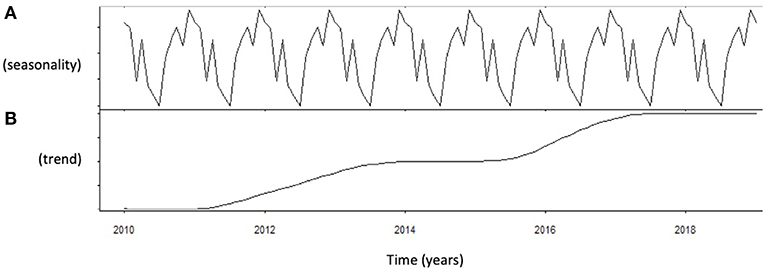
Figure 1. Analysis of serum testosterone level distribution using autoregressive integrated moving average (ARIMA) model. (A) Shows the data distribution across years, suggesting possible peak and nadir. (B) Shows the trend of data collected across years of observation.
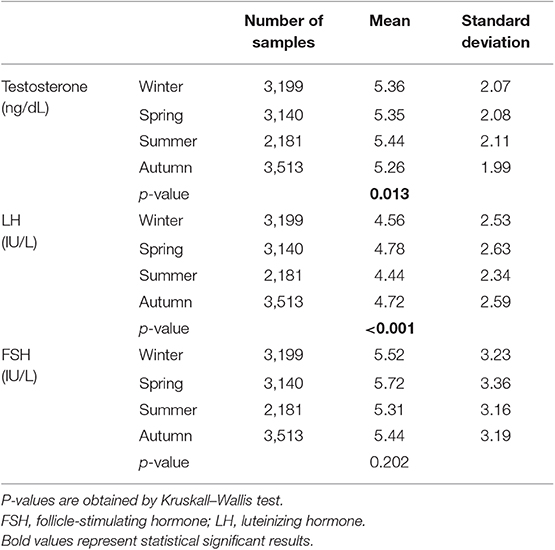
Table 1. Hormone serum levels in the four seasons across the study years.
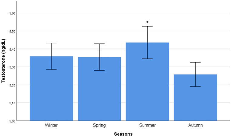
Figure 2. Comparison of mean testosterone serum levels among seasons. Comparison was performed by Kruskal-Wallis test. *Identifies the highest testosterone serum levels at post hoc Tukey test.
Autocorrelation function was applied to LH distribution, identifying two significant peaks followed by a long exponential tail, typical of historical series (peak 1: 0.216, standard error 0.009, coefficient 562.7, Box-Ljung test, p < 0.001; peak 2: 0.108, standard error 0.009, coefficient 1928.0, Box-Ljung test, p < 0.001). This double peak was confirmed using the Wilcoxon Signed Rank test (p = 0.001), confirming the seasonal LH distribution. Seasonal decomposition was applied with ARIMA (0,0,0), detecting mean value 3.91 and standard error 0.54, sigma2 estimated 3.29 with log likelihood = −19.62, AIC = 43.23, and BIC = 43.84. LH did not show any significant trend across the years (Figure 3B). This result was confirmed considering only the last year of observation (sigma2 estimated 3.11 with log likelihood = −18.30). A seasonal distribution was evident (Figure 3A), with two annual peaks. Mean LH levels confirmed a different distribution among the seasons (p < 0.001), with two peaks per year, in spring and autumn, respectively (Figure 4, Table 1). Indeed, LH serum levels were significantly higher in spring compared to summer and winter (p = 0.004 and p < 0.001, respectively) and in autumn compared to winter and summer (p = 0.044 and p < 0.001, respectively) (Figure 4, Table 1).
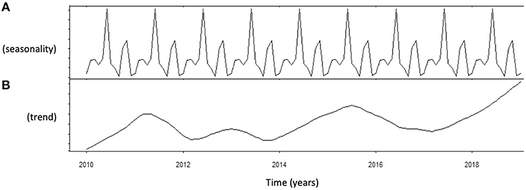
Figure 3. Analysis of luteinizing hormone (LH) levels distribution using autoregressive integrated moving average (ARIMA) model. (A) Shows the data distribution across years, suggesting possible peak and nadir. (B) Shows the trend of data collected across years of observation.
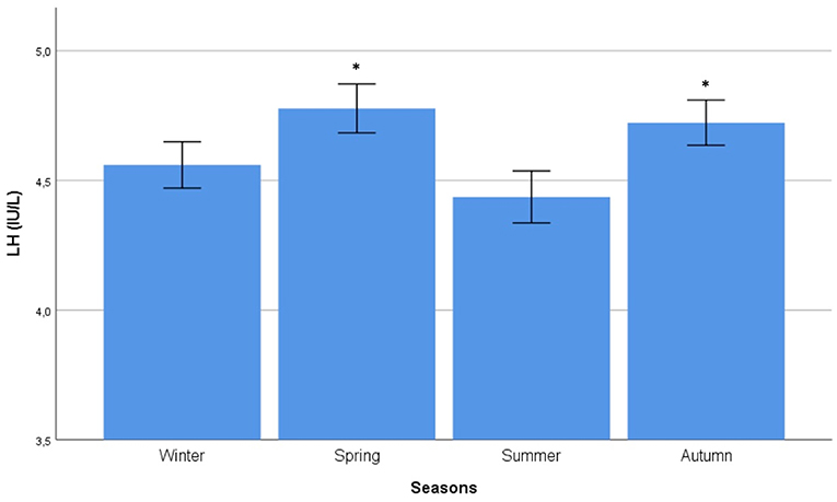
Figure 4. Comparison of mean luteinizing hormone (LH) serum levels among seasons. Comparison was performed by Kruskal–Wallis test. *Identifies the highest LH serum levels at post hoc Tukey test.
Considering FSH, no significant peaks were detected by autocorrelation functions. As a confirmation, ARIMA did not highlight any seasonal distribution of FSH (mean 3.82, standard error 0.44, sigma2 estimated 2.14, log likelihood = −17.47, AIC = 38.93 and BIC = 39.54), and the Box-Ljung test did not detect any significant seasonal distribution (X-squared = 9.44, degrees of freedom = 8, p = 0.306). Mean FSH levels differences among seasons confirmed the lack of seasonality (p = 0.202) (Table 1).
Considering patients' age, the following quartiles were created: (i) from 18 to 35 years (group 1 – 3145 data), (ii) from 35.1 to 48 years (group 2 2880 data), (iii) from 48.1 to 57 years (group 3 – 3310 data), and (iv) older than 57.1 years (group 4 – 2698 data). In the first group, LH and testosterone did not differ among seasons (p = 0.773 and p = 0.301, respectively). In group 2, LH was significantly different among seasons (p < 0.001), confirming the highest levels in spring and autumn (p < 0.001 and p = 0.005, respectively). However, annual peak of testosterone was not confirmed (p = 0.060). In group 3, the seasonal differences of both testosterone and LH were confirmed (p = 0.004 and p = 0.002, respectively). At post hoc analysis, the highest testosterone levels were detected in summer (p = 0.002) and the highest LH levels in spring and autumn (p = 0.004 and p = 0.006, respectively). Finally, in group 4, no seasonal differences were detected, neither for testosterone nor for LH (p = 0.155 and p = 0.080, respectively).
Considering semen analyses, sperm concentration was used to evaluate seasonality. Autocorrelation function did not detect significant peaks and no seasonality was detected at Box-Ljung test (p = 0.402). Finally, PRL did not show any seasonal fluctuation (p = 0.421), without significant differences among seasons (p = 0.181).
Correlations Among Hormones
Patients' age was inversely related to serum testosterone levels (R = −0–148, p < 0.001) and directly related to LH (R = 0.185, p < 0.001) and FSH (R = 0.281, p < 0.001). As expected, total testosterone serum levels were directly related to LH (R = 0.147, p < 0.001), but not to FSH (R = −0.006, p = 0.482). Finally, LH was directly related to FSH (R = 0.538, p < 0.001). The internal 5-fold cross-validation method confirmed the significant result obtained by conventional statistical analyses. No correlations among semen parameters and sexual hormones were detected.
Environmental Influence on Seasonality
Testosterone serum levels were within the laboratory reference range (2.2–8.7 ng/dL) in 10,905 patients (90.6%), while 311 patients (2.6%) and 817 patients (6.8%) showed testosterone levels lower and higher than the reference range. Although testosterone seasonality remained statistically significant considering only data within the reference range, a significant zenith was not detected by mean differences among seasons (p = 0.288) (Table 2), suggesting that the significant seasonal variability is evident including values that are outside the laboratory reference range. On the contrary, LH seasonality was confirmed for data within the reference range (1–9 IU/L) and higher levels were confirmed in spring and autumn (Table 2) (p = 0.001).
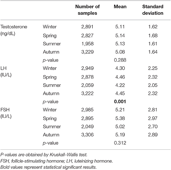
Table 2. Hormone serum levels in the four seasons across the study years considering only hormones within the laboratory reference ranges.
PRL serum levels did neither correlate with testosterone (Rho: 0.002, p = 0.804), nor LH (Rho: 0.005, p = 0.665) nor FSH (Rho: 0.006, p = 0.734). Serum total testosterone was directly related to maximum, minimum and mean daily temperatures (Rho: 0.019—p = 0.041, Rho: 0.023—p = 0.011, and Rho: 0.021—p = 0.024, respectively) (Figure 5), but not to humidity (Rho: −0.009, p = 0.340). Moreover, testosterone was directly related to daylight duration (Rho: 0.021—p = 0.020). LH was directly related to minimum temperatures (Rho: −0.022—p = 0.018), but not to maximum and mean temperatures, humidity and daylight duration (Rho: 0.012—p = 0.173, Rho: 0.016—p = 0.089, Rho: 0.012—p = 0.202, and Rho: 0.007 – p = 0–467, respectively). The cross-validation method confirmed the significant correlations, apart from the correlation between LH and minimum temperatures. Indeed, after cross-validation, this correlation was lacking, suggesting that the large amount of data biased this correlation. FSH was not related to environmental parameters. Finally, after seasonal decomposition, environmental temperatures (maximum, minimum and mean temperatures) showed a significant increasing trend across years (p < 0.001). In particular, the mean yearly temperature passed from 13.13 ± 8.28 °C in 2010 to 14.61 ± 7.81 °C in 2018. Thus, the increasing trend detected in testosterone distribution could be related to the increasing environmental temperature.
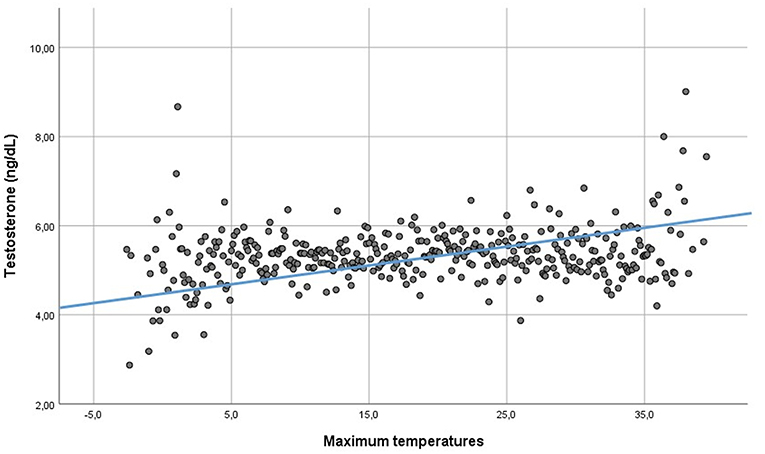
Figure 5. Linear regression between testosterone serum levels and environmental maximum temperatures.
Discussion
We demonstrate a clear seasonal fluctuation of both LH and testosterone in a large sample of adult human males. As expected, testosterone appears directly related to LH, but the annual fluctuation of these two hormones is not synchronous. LH shows a bi-annual fluctuation, with two peaks reached in spring and autumn, while testosterone shows only one summer peak. Moreover, the testosterone annual change shows a wider variability in annual values compared to LH, evident including levels below and above the laboratory reference ranges, while LH fluctuations remain irrespective of the reference range. Interestingly, the testosterone zenith is reached at least 3 months after the LH peak, a possible late consequence of the vernal LH peak. However, should this rhythmicity reflect a connection between the pituitary gland and the testicle, we should find two testosterone peaks every year. Rather, testosterone seasonal fluctuation could be mainly influenced by the environment. In particular, we show here an increasing trend of environmental temperatures across the years of observation, related to increasing testosterone serum levels. Moreover, when temperatures are higher during the year and the daylight duration is the longest (i.e., summer), testosterone serum levels reach their annual zenith. On the contrary, LH seasonality seems to be independent from environment, and a central mechanism, possibly regulating seasonal fluctuations of the hypothalamic gonadotropin-releasing hormone (GnRH), might be involved. It is well-known that LH secretion is the result of GnRH pulsatility, regulated by hypothalamic clock genes from one side (22) and pulsatile secretion of Kisspeptin on the other side (23), which is the main regulatory mechanism of GnRH secretion in vertebrates (24, 25). In seasonally breeding animals, the circadian and photoperiodic regulation of the neuroendocrine system is largely demonstrated to modulate diurnal and semilunar spawning rhythm (23). Similarly, a complex regulation of hormonal seasonality, involving the pineal pulse generator, is suggested in humans (26). In particular, the melatonin secretory cyclic pattern seems to be sufficient to compensate the physiological secretory pattern which is lacking in men with congenital GnRH deficiency (26). Our study does not show any influence of daylight duration on LH secretion, suggesting a mechanism probably independent from melatonin.
In the literature, 15 clinical trials investigated testosterone seasonality (Table 3). Ten studies detected testosterone fluctuations along the year (66.7%) (28–30, 35–41), with an annual pattern of testosterone secretion highlighted in most cases, and a bi-annual pattern detected only in 3 out of 10 studies (Table 3), whereas 5 did not (27, 31–34). Almost all previous studies evaluated small groups of men and only 3 studies considered more than one thousand subjects. Moreover, two of the most numerous casuistries enrolled older (32) and younger (30) men separately, whereas in our study we cover the entire life-time after puberty, from 18 to 91 years. Only Svartberg et al. evaluated a large cohort including men of all ages older than 25 years (41). However, the seasonal evaluation was limited to testosterone serum levels. A comprehensive assessment of the seasonal rhythmicity of the pituitary-gonadal axis requires not only a high number of adult patients without age limits but also all hormones involved. In our study we could evaluate how the seasonal hormonal changes were affected by age. Indeed, dividing the entire cohort of patients according to age, we highlight seasonal changes in men between 35 and 57 years, whereas no seasonal effect seems evident for men younger than 35 years or older than 57 years. This finding is novel and could explain the discrepancies of the results reported in the earlier literature. Hormones seasonality is lost after 57 years, when a progressive decline of testosterone occurs, probably limiting the yearly change (42).
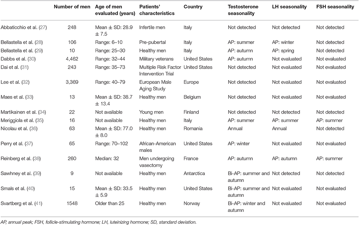
Table 3. Published trials on testosterone seasonality.
The seasonal variability could be due to environmental influence on the reproductive system (4). Available studies evaluating testosterone fluctuations are not homogeneously distributed across the world and only few latitudes have been studied so far. In this context, the lack of sun exposure for a long period of the year, as observed at high latitude countries (34, 39, 41), could represent a confounding factor in evaluating the hormonal seasonality. Indeed, daily hours of sunshine, minimum and maximum temperatures and humidity were demonstrated to influence annual rhythms of human reproduction already in the 1930s (4) and a relationship between testosterone and melatonin secretion has been suggested (43). However, after industrialization, humans are progressively and increasingly shielded from both daylight duration by indoor work, and environmental temperature by heating and air conditioning. These changes in life habits might result in a “de-seasonalization” of human reproduction and possibly in testosterone fluctuation. However, as shown in the majority of industrialized populations studied so far, we confirm the persistence of an annual pattern of testosterone fluctuation. Moreover, we confirm the correlation between testosterone and environmental temperatures, considering maximum, minimum and mean daily values. Increasing environmental temperatures, testosterone raises, reaching the highest values in summer. In this setting, there is large evidence of the detrimental effect of local heat on Leydig cells activity and survival in animal models (44, 45). In particular, heat-induced testicular damage is mediated by the activation of specific apoptotic pathways in animal models (46, 47). However, less is known about the possible effect of environmental temperature on Leydig cells activity in humans. Here we detect a direct linear correlation between testosterone and environmental temperatures, suggesting that low environmental temperatures may be less favorable for testicular steroidogenesis.
Apart from the seasonal fluctuation, testosterone showed a significant increasing trend during years, from 2010 to 2018. This trend could be explained by the increasing environmental temperatures, recorded in the years of the study. Indeed, we demonstrated a direct relationship between testosterone and environmental temperatures in our cohort. Accordingly, environmental temperatures increased in the 9-years interval of the study, with a mean increase of 1.48°C. This increase goes along with a mean testosterone increase of 0.44 ng/dL detected after 9 years of evaluation.
In our cohort, FSH does not fluctuate and a seasonal change in sperm parameter is not detected. However, semen analyses were available only in 2.6% of the entire group, limiting the statistical power. Indeed, increasing the sample size (5,573 semen analyses), we previously detected semen seasonality, with higher sperm number in winter/spring seasons compared to summer/autumn (48). Moreover, in this previous work, a significant correlation between semen analyses and environmental parameters was evident (48). Thus, a larger dataset, containing both semen analyses and hormone evaluations, is needed to completely understand the environmental influence on reproduction along the seasons.
Our study has some strengths. We evaluated (i) a large number of men, (ii) living at the same latitude, (iii) in a long time-frame interval, (iv) without known diseases affecting the hypothalamic-pituitary-gonadal axis, and (v) considering both testosterone and gonadotropins serum levels. However, several limitations should be considered. First, patients were evaluated only once, thus a longitudinal evaluation of testosterone changes in the same patient is not possible. Second, testosterone serum levels were assayed using commercially available kits and not the gold-standard liquid-chromatography tandem mass-spectrometry (LC-MS/MS). Third, no information is available about liver function. Thus, we are not able to consider possible sex hormone binding globulin (SHBG) changes and, consequently, whether these fluctuations are reflected in a seasonal variation of bioavailable testosterone. Finally, semen analyses were available only in a small subgroup of patients and an overall assessment of the seasonality of FSH and semen parameters together is prevented. An accurate evaluation of the seasonal influence on spermatogenesis could elucidate the possible residual role of environmental exposure in terms of reproductive advantage. In this context, the coeval fluctuation of androgens could be involved, maybe influencing libido to optimize conceptions.
Conclusions
In conclusion, our results demonstrate biannual/circannual fluctuations of serum LH and testosterone, suggesting a seasonal influence on the pituitary-gonadal axis in the human species. The circannual testosterone and LH fluctuation is possibly subjected to different regulation mechanisms (central for LH vs. environmental for testosterone). Considering the limited amplitude of the testosterone and LH fluctuation across the year, the absence of seasonality in the youngest and oldest age groups, and the reduced exposure to environmental factors in the industrialized era, we could speculate that the ancestral secretory pattern adaptive toward seasons in various animal species is (gradually?) disappearing in the human.
Data Availability Statement
The data that support the findings of this study are available on request from the corresponding author. The data are not publicly available due to privacy or ethical restrictions.
Ethics Statement
Ethical approval was not provided for this study on human participants because considering the retrospective, big data study design, it was not possible to obtain informed consent from all participants included in the study, but all examinations were approved by the Ospedale Civile of Baggiovara management, since data were collected anonymously. Written informed consent for participation was not required for this study in accordance with the national legislation and the institutional requirements.
Author Contributions
DS conceived the study, analyzed the data, and wrote the manuscript. GS analyzed the data and wrote the manuscript. MSe coordinated the data extraction. ST and TT performed laboratory assays. AG and MSi contributed wrote the manuscript. All authors edited the manuscript or revised it critically for important intellectual content and approved the final draft.
Conflict of Interest
The authors declare that the research was conducted in the absence of any commercial or financial relationships that could be construed as a potential conflict of interest.
References
1. Minors DS, Waterhouse JM. Anchor sleep as a synchronizer of rhythms on abnormal routines. Int J Chronobiol. (1981) 7:165–88.
2. Minors DS, Waterhouse JM. Endogenous and exogenous components of circadian rhythms when living on a 21-hour day. Int J Chronobiol. (1981) 8:31–48.
3. Wehr TA. Photoperiodism in humans and other primates: evidence and implications. J Biol Rhythms. (2001) 16:348–64. doi: 10.1177/074873001129002060
4. Roenneberg T, Aschoff J. Annual rhythm of human reproduction: II. Environmental correlations J Biol Rhythms. (1990) 5:217–39. doi: 10.1177/074873049000500304
5. Dunlap JC. Molecular bases for circadian clocks. Cell. (1999) 96:271–90. doi: 10.1016/S0092-8674(00)80566-8
6. Doi M, Hirayama J, Sassone-Corsi P. Circadian regulator CLOCK is a histone acetyltransferase. Cell. (2006) 125:497–508. doi: 10.1016/j.cell.2006.03.033
7. Hirayama J, Sahar S, Grimaldi B, Tamaru T, Takamatsu K, Nakahata Y, et al. CLOCK-mediated acetylation of BMAL1 controls circadian function. Nature. (2007) 450:1086–90. doi: 10.1038/nature06394
8. Dibner C, Schibler U, Albrecht U. The mammalian circadian timing system: organization and coordination of central and peripheral clocks. Annu Rev Physiol. (2010) 72:517–49. doi: 10.1146/annurev-physiol-021909-135821
9. Li Y, Li G, Wang H, Du J, Yan J. Analysis of a gene regulatory cascade mediating circadian rhythm in zebrafish. PLoS Comput Biol. (2013) 9:e1002940. doi: 10.1371/journal.pcbi.1002940
10. Kovanen L, Saarikoski ST, Aromaa A, Lonnqvist J, Partonen T. ARNTL, (BMAL1) and NPAS2 gene variants contribute to fertility and seasonality. PLoS ONE. (2010) 5:e10007. doi: 10.1371/journal.pone.0010007
11. Urbanski HF. Role of circadian neuroendocrine rhythms in the control of behavior and physiology. Neuroendocrinology. (2011) 93:211–22. doi: 10.1159/000327399
13. Jensen RL, Kline GM. The resampling cross-validation technique in exercise science: modelling rowing power. Med Sci Sports Exerc. (1994) 26:929–33. doi: 10.1249/00005768-199407000-00019
14. Shimodaira H. Cross-validation of matching correlation analysis by resampling matching weights. Neural Netw. (2016) 75:126–40. doi: 10.1016/j.neunet.2015.12.007
15. Ke Z, Zhang ZJ. Testing autocorrelation and partial autocorrelation: asymptotic methods versus resampling techniques. Br J Math Stat Psychol. (2018) 71:96–116. doi: 10.1111/bmsp.12109
16. Batt RD, Eason T, Garmestani A. Time scale of resilience loss: implications for managing critical transitions in water quality. PLoS ONE. (2019) 14:e0223366. doi: 10.1371/journal.pone.0223366
17. Box GE, Jenkins GM. Time Series Analysis: Forecasting and Control. Englewood Cliffs: Prentice Hall (1994).
19. Jain RK, Sharma RD, Jain S. Application of ARIMA model in adjustment of seasonal and non-seasonal variations in births of Ontario. Genus. (1985) 41:127–33.
20. Jensen L. Guidelines for the application of ARIMA models in time series. Res Nurs Health. (1990) 13:429–35. doi: 10.1002/nur.4770130611
21. Delavary Foroutaghe M, Mohammadzadeh Moghaddam A, Fakoor V. Time trends in gender-specific incidence rates of road traffic injuries in Iran. PLoS ONE. (2019) 14:e0216462. doi: 10.1371/journal.pone.0216462
22. Simoni M, Montanini V, Fustini MF, Del Rio G, Cioni K, Marrama P. Circadian rhythm of plasma testosterone in men with idiopathic hypogonadotrophic hypogonadism before and during pulsatile administration of gonadotrophin-releasing hormone. Clin Endocrinol. (1992) 36:29–34. doi: 10.1111/j.1365-2265.1992.tb02899.x
23. Ando H, Ogawa S, Shahjahan M, Ikegami T, Doi H, Hattori A, et al. Diurnal and circadian oscillations in expression of kisspeptin, kisspeptin receptor and gonadotrophin-releasing hormone 2 genes in the grass puffer, a semilunar-synchronised spawner. J Neuroendocrinol. (2014) 26:459–67. doi: 10.1111/jne.12165
24. Hussain MA, Song WJ, Wolfe A. There is kisspeptin - and then there is kisspeptin. Trends Endocrinol Metab. (2015) 26:564–72. doi: 10.1016/j.tem.2015.07.008
25. Ando H, Shahjahan M, Kitahashi T. Periodic regulation of expression of genes for kisspeptin, gonadotropin-inhibitory hormone and their receptors in the grass puffer: implications in seasonal, daily and lunar rhythms of reproduction. Gen Comp Endocrinol. (2018) 265:149–53. doi: 10.1016/j.ygcen.2018.04.006
26. Luboshitzky R, Herer P, Lavie P. Pulsatile patterns of melatonin secretion in patients with gonadotropin-releasing hormone deficiency: effects of testosterone treatment. J Pineal Res. (1997) 22:95–101. doi: 10.1111/j.1600-079X.1997.tb00309.x
27. Abbaticchio G, de Fini M, Giagulli VA, Santoro G, Vendola G, Giorgino R. Circannual rhythms in reproductive functions of human males, correlations among hormones and hormone-dependent parameters. Andrologia. (1987) 19:353–61. doi: 10.1111/j.1439-0272.1987.tb02314.x
28. Bellastella A, Criscuolo T, Mango A, Perrone L, Sinisi AA, Faggiano M. Circannual rhythms of plasma luteinizing hormone, follicle-stimulating hormone, testosterone, prolactin and cortisol in prepuberty. Clin Endocrinol. (1983) 19:453–9. doi: 10.1111/j.1365-2265.1983.tb00019.x
29. Bellastella G, Pane E, Iorio S, De Bellis A, Sinisi AA. Seasonal variations of plasma gonadotropin, prolactin, and testosterone levels in primary and secondary hypogonadism: evidence for an independent testicular role. J Endocrinol Invest. (2013) 36:339–42. doi: 10.3275/8620
30. Dabbs JM Jr. Age and seasonal variation in serum testosterone concentration among men. Chronobiol Int. (1990) 7:245–9. doi: 10.3109/07420529009056982
31. Dai WS, Kuller LH, LaPorte RE, Gutai JP, Falvo-Gerard L, Caggiula A. The epidemiology of plasma testosterone levels in middle-aged men. Am J Epidemiol. (1981) 114:804–16. doi: 10.1093/oxfordjournals.aje.a113251
32. Lee DM, Tajar A, Pye SR, Boonen S, Vanderschueren D, Bouillon R, et al. Association of hypogonadism with vitamin D status: the European Male Ageing Study. Eur J Endocrinol. (2012) 166:77–85. doi: 10.1530/EJE-11-0743
33. Maes M, Mommen K, Hendrickx D, Peeters D, D'Hondt P, Ranjan R, et al. Components of biological variation, including seasonality, in blood concentrations of TSH, TT3, FT4, PRL, cortisol and testosterone in healthy volunteers. Clin Endocrinol. (1997) 46:587–98. doi: 10.1046/j.1365-2265.1997.1881002.x
34. Martikainen H, Tapanainen J, Vakkuri O, Leppaluoto J, Huhtaniemi I. Circannual concentrations of melatonin, gonadotrophins, prolactin and gonadal steroids in males in a geographical area with a large annual variation in daylight. Acta Endocrinol. (1985) 109:446–50. doi: 10.1530/acta.0.1090446
35. Meriggiola MC, Noonan EA, Paulsen CA, Bremner WJ. Annual patterns of luteinizing hormone, follicle stimulating hormone, testosterone and inhibin in normal men. Hum Reprod. (1996) 11:248–52. doi: 10.1093/HUMREP/11.2.248
36. Nicolau GY, Haus E, Lakatua DJ, Bogdan C, Sackett-Lundeen L, Popescu M, et al. Circadian and circannual variations of FSH, LH, testosterone, dehydroepiandrosterone-sulfate (DHEA-S), and 17-hydroxy progesterone, (17 OH-Prog) in elderly men and women. Endocrinologie. (1985) 23:223–46.
37. Perry HMIII, Miller DK, Patrick P, Morley JE. Testosterone and leptin in older African-American men: relationship to age, strength, function, and season. Metabolism. (2000) 49:1085–91. doi: 10.1053/meta.2000.7710
38. Reinberg A, Smolensky MH, Hallek M, Smith KD, Steinberger E. Annual variation in semen characteristics and plasma hormone levels in men undergoing vasectomy. Fertil Steril. (1988) 49:309–15. doi: 10.1016/S0015-0282(16)59721-0
39. Sawhney RC, Malhotra AS, Prasad R, Pal K, Kumar R, Bajaj AC. Pituitary-gonadal hormones during prolonged residency in Antarctica. Int J Biometeorol. (1998) 42:51–4. doi: 10.1007/s004840050083
40. Smals AG, Kloppenborg PW, Benraad TJ. Circannual cycle in plasma testosterone levels in man. J Clin Endocrinol Metab. (1976) 42:979–82. doi: 10.1210/jcem-42-5-979
41. Svartberg J, Jorde R, Sundsfjord J, Bonaa KH, Barrett-Connor E. Seasonal variation of testosterone and waist to hip ratio in men: the Tromso study. J Clin Endocrinol Metab. (2003) 88:3099–104. doi: 10.1210/jc.2002-021878
42. Zirkin BR, Tenover JL. Aging and declining testosterone: past, present, and hopes for the future. J Androl. (2012) 33:1111–8. doi: 10.2164/jandrol.112.017160
43. Luboshitzky R, Levi M, Shen-Orr Z, Blumenfeld Z, Herer P, Lavie P. Long-term melatonin administration does not alter pituitary-gonadal hormone secretion in normal men. Hum Reprod. (2000) 15:60–5. doi: 10.1093/humrep/15.1.60
44. Kanter M, Aktas C. Effects of scrotal hyperthermia on Leydig cells in long-term: a histological, immunohistochemical and ultrastructural study in rats. J Mol Histol. (2009) 40:123–30. doi: 10.1007/s10735-009-9222-5
45. Kim JH, Park SJ, Kim TS, Kim JM, Lee DS. Testosterone production by a Leydig tumor cell line is suppressed by hyperthermia-induced endoplasmic reticulum stress in mice. Life Sci. (2016) 146:184–91. doi: 10.1016/j.lfs.2015.12.042
46. Yin Y, DeWolf WC, Morgentaler A. Experimental cryptorchidism induces testicular germ cell apoptosis by p53-dependent and -independent pathways in mice. Biol Reprod. (1998) 58:492–6. doi: 10.1095/biolreprod58.2.492
47. Yin Y, Stahl BC, DeWolf WC, Morgentaler A. P53 and Fas are sequential mechanisms of testicular germ cell apoptosis. J Androl. (2002) 23:64–70. doi: 10.1002/jand.2002.23.1.64
Keywords: luteinizing hormone, follicle stimulating hormone, testosterone, seasonal variation, daylight cycle
Citation: Santi D, Spaggiari G, Granata ARM, Setti M, Tagliavini S, Trenti T and Simoni M (2020) Seasonal Changes of Serum Gonadotropins and Testosterone in Men Revealed by a Large Data Set of Real-World Observations Over Nine Years. Front. Endocrinol. 10:914. doi: 10.3389/fendo.2019.00914
Received: 31 July 2019; Accepted: 16 December 2019;
Published: 10 January 2020.
Edited by:
Ren-Shan Ge, Wenzhou Medical University, ChinaReviewed by:
Watanabe Gen, Tokyo University of Agriculture and Technology, JapanPeter Stanton, Hudson Institute of Medical Research, Australia
Copyright © 2020 Santi, Spaggiari, Granata, Setti, Tagliavini, Trenti and Simoni. This is an open-access article distributed under the terms of the Creative Commons Attribution License (CC BY). The use, distribution or reproduction in other forums is permitted, provided the original author(s) and the copyright owner(s) are credited and that the original publication in this journal is cited, in accordance with accepted academic practice. No use, distribution or reproduction is permitted which does not comply with these terms.
*Correspondence: Daniele Santi, daniele.santi@unimore.it
†ORCID: Daniele Santi orcid.org/0000-0001-6607-7105