The Optimal Design of a Distillation System for the Flexible Polygeneration of Dimethyl Ether and Methanol Under Uncertainty

Introduction

Flexible Polygeneration

Colloquially, the term polygeneration refers to chemical plants that generate more than one kind of product. However, a recent review of polygeneration concluded that, in practice, the term in the taxonomical sense refers to chemical plants that produce electricity and at least one kind of chemical product, and also do not fall into other taxonomies such as biorefinery, co-generation, tri-generation, or petrochemical refinery (Adams and Ghouse, 2015). The reason for this is in large part because of the nature of chemical processing and its relationship to economics. If the goal of a company is to produce both chemicals A and B continuously and in particular amounts, a company could choose to create two chemical plants independent from each other, one that always produces A and one that always produces B. However, if A and B have some common upstream processing steps, for example, sharing the same intermediate reaction steps or reagents, then there is significant benefit to integrating the two into a polygeneration process with one common upstream step to produce those intermediate components and two separate downstream processing steps that produce the different chemicals A and B. A common example might be where A and B are chemicals that are made via the syngas route (syngas being the common intermediate), such as methanol, dimethyl ether, synthetic transportation fuels, olefins, aromatics, ethanol, etc. (Chen et al., 2011b). This is usually what is meant colloquially by polygeneration. The primary benefit here is usually economy of scale of the shared upstream portion. It is usually much less expensive to have one process train at a large capacity than to have two process trains of half the capacity in parallel.

However, when the goal of the company is not to make certain amounts of A and B, but to make whichever combination is the most profitable or the best investment, the resulting design is very different. A review of studies of this optimal polygeneration problem found that overwhelmingly, the optimal chemical process was the one that produced only A or B, but not both, with the choice determined by expected market conditions (Adams and Ghouse, 2015). In most studies, there simply just was not enough synergy to exploit between the two downstream process trains for A and B such that there was any financial reason to produce both A and B when only one would do. Usually, there happened to be sufficient waste gases produced from the production of the chemical to be used for electricity production in meaningful quantities. These results were so common across researchers that the term polygeneration in the taxonomical sense was defined to be the co-production of electricity and only a minimum of one chemical or fuel product, not two.

However, because market conditions can change frequently and significantly over the many decades a large-scale chemical plant is expected to operate, there is a substantial incentive for flexible polygeneration. This is the idea that a chemical plant is designed with the capability of producing both A and B, but then the amounts of A or B produced are changed at various times in the lifetime of the plant depending on the market conditions at the time. This essentially amounts to overdesigning the system, creating extra capacity which will never be fully used at any given time but having it ready for when the time is right. Despite the very high capital cost this approach, the net financial benefits of this can be very significant, with one study putting the upper bound for a plant of industrially relevant size at a 63% boost in net present value (NPV) compared to a static polygeneration plant, worth up to $1 billion in extra net value (Chen et al., 2011a).

Even so, flexible polygeneration optimization research results usually show that, in the general case, it is still better to produce either entirely A or entirely B at any one time, and then switch completely between them when market conditions shift between certain critical points (Chen et al., 2012). The only exceptions are usually when there are limits to the turndown ratio (the amount that a process train can be turned down before it becomes too hard to turn it back up again without major expense), or when the problem is otherwise somewhat arbitrarily imposed with constraints that require a certain minimum amount of each product to be made at any given time, or when there is a fixed upper limit on capital expenditure. These constraints are commonly imposed in academic studies precisely to arrive at solutions that do not completely eliminate one of the chemicals in order to make the results more interesting. Even so, the optimal flexible solution is to maximize the production of one chemical and minimize the other at any one time depending on current market condition.

In all of the above cases, these optimization results are a direct result of the inherent nature of the design itself, in which each chemical train is decoupled from the others in the downstream portion due to a lack of meaningful process synergies between them. All of the advantages of flexible polygeneration arise from a combination of the shared upstream components and the ability to profit from market volatility, rather than any synergy exploitation between process trains. However, in this work, we examine how there are synergies that can be exploited between process trains in some cases by looking at the level of the individual equipment. For example, if the trains for chemical A and chemical B both use distillation columns, and since we know from the survey of the literature that the optimum flexible polygeneration process tends to operate with only one kind of product at a time, we can then design flexible distillation columns which could be used for different purposes depending whether we were currently producing A or B. The principle here is that instead of constructing two separate column sequences for train A and train B that are each used only a portion of their lifetime, we construct just one distillation sequence and use it at all times, albeit for different purposes. This may of course mean that it is optimal or inefficient at any one time, but on the whole, the savings from constructing only half as many columns might be a sufficient cost incentive.

This work examines this idea and quantifies the benefit of this flexible design for an illustrative case study. One key challenge is that in order to do this, there must be a sufficiently rigorous model in place, which can make optimization difficult. Note that most flexible polygeneration optimization studies use reduced or lumped models for process units or sections, which is reasonable in those cases when process trains are uncoupled. In addition, the optimal design of this flexible distillation system is now dependent on expected market conditions. For example, if one expected to make chemical A for the majority of the process lifetime and spend only a small amount of time making chemical B, one might design the columns to be very efficient at making chemical A knowing full well that although it was inefficient at making B, this will happen infrequently. On the other hand, if you expect to make about as much A as B over the lifetime of the plant, then perhaps a more balanced design is more economical. Thus, the problem of designing this flexible distillation system is coupled with the consideration of market expectation and therefore market uncertainty in order to be meaningful.

This work presents an optimization framework and method which can be used to tackle this problem quickly and quantifies the benefits of this integration. To the authors' knowledge, it is the first work concerning optimal flexible polygeneration that examines integration at the individual equipment level with rigorous unit operation models and no shortcut approximations when considering integer variables. It achieves this by reducing all uncertainty related to future markets and business behavior to one uncertainty variable and by decomposing the problem into small, tractable pieces. It is also the first such work for DME and Methanol.

Flexible Design Under Uncertainty

Process plants typically operate in an environment of change (such as feed type and rate, and market conditions), often coupled with uncertainty. A design that is optimal under nominal conditions may be grossly suboptimal, or even infeasible, as process conditions change. This has led to the development of design formulations in which change and uncertainty are directly taken into account.

Grossmann and coworkers (Halemane and Grossmann, 1983; Swaney and Grossmann, 1985) define flexibility in design as the ability to maintain feasible operation over a range of uncertain parameter realizations, and proposed a mathematical formulation and solution strategies for flexibility assessment. An important feature of their formulation is its allowance for adjustment of operating conditions through control variables for a given uncertain parameter realization. Extensions of the method include alternative solution strategies (Grossmann and Floudas, 1987), application to dynamic systems (Dimitriadis and Pistikopoulos, 1995) and consideration of joint confidence regions of uncertain parameters (Rooney and Biegler, 1999). Several applications have been reported, including flexibility analysis of air separation systems (Sirdeshpande et al., 2005), plant waste management policies (Chakraborty and Linninger, 2003), and process supply chain networks (Wang et al., 2016). A recent review of the flexibility analysis framework is given in Grossmann et al. (2014).

The above described flexibility analysis framework has parallels with two-stage stochastic optimization (Birge and Louveau, 1997) that has been quite widely applied to design under uncertainty. Here, decision variables are partitioned into first-stage decision variables that are made prior to the uncertain event taking place, and second-stage or recourse decisions that are made in response to uncertainty realizations. A widely used implementation strategy is to discretize the uncertainty region to yield a multiscenario optimization formulation. Within a plant design context, first-stage decisions are typically associated with design variables that are fixed throughout the horizon under consideration, and second-stage decisions with operating or control variables than can be changed in response to varying conditions. Zhu et al. (2010) apply a two-stage stochastic formulation to the design of a cryogenic air separation unit in which uncertainty in demand and a physical property parameter is considered. Five first-stage design variables are considered, and five control variables are selected to compensate for variation in product demand. Liu et al. (2010) present a two-stage stochastic formulation for polygeneration energy systems, and apply a decomposition strategy to solve the resulting multiperiod optimization problem. Chen et al. (2011a) formulate the design of a flexible polygeneration system under market uncertainty as a two-stage stochastic programming problem, and demonstrate superior net present values of flexible designs over static designs. In Chen et al. (2012) a decomposition strategy is proposed for global solution of the flexible design problem, which yields significantly faster solutions than a commercial global optimization solver. Two-stage stochastic programming has also been quite widely applied to supply chain operation and design. This includes contributions in supply chain planning under uncertainty (Gupta and Maranas, 2003), multi-echelon supply chain network design under uncertainty (Tsiakis et al., 2001), and dynamic operability analysis of process supply chain systems (Mastragostino and Swartz, 2014). An overview of two-stage stochastic programming formulations, solution approaches, and process systems applications is given in Grossmann et al. (2016).

In this work, we explore flexible distillation design configurations for two feed conditions (parameter realizations), and thereafter investigate a scenario-based two-stage stochastic formulation for consideration of uncertainty in the total length of time that the distillation systems process the specific feed types. This uncertainty parameter is used to describe all unknown factors that would impact the operating decision to produce one product versus another at any given time, including market conditions and other external factors. This work does not explore uncertainty in the model parameters. Although uncertainty in parameters such as thermodynamic properties (Whiting, 1996), phase equilibria (Burger and Schwarz, 2018), or process model-mismatch play a role in any process design problem, the focus in this work is on uncertainty in operational decision factors.

Case Study

Flexible Base Case Design

In this work, we consider the production of DME from syngas through the two-step route, as shown in Figure 1. Synthesis gas (or “syngas”) is produced from the gasification of coal, biomass, or petcoke, or via methane reforming (or some combination thereof) such that after certain cleaning steps (such as the removal of water, CO₂, H₂S, and various pollutants), the syngas is composed of a mixture of H₂ and CO with a molar H₂:CO ratio of about 2:1. Although it is possible to produce DME directly in a single reactor (Ogawa et al., 2003) or through catalytic distillation (An et al., 2004; Kiss and Suszwalak, 2012), for the purposes of this example, we have chosen the two-step route in which methanol is first produced from the syngas and then DME is dehydrated from the methanol (Xu et al., 1997). For the flexible polygeneration base case, the product stream from the first reactor can optionally be either sent in total to the DME synthesis reactor when in “Maximize DME Mode,” or, to a distillation sequence for purification when in “Maximize Methanol Mode.” Everything upstream of this decision point is always operating at the same condition. During the DME Mode the DME reactor output is sent to a different distillation sequence.

FIGURE 1

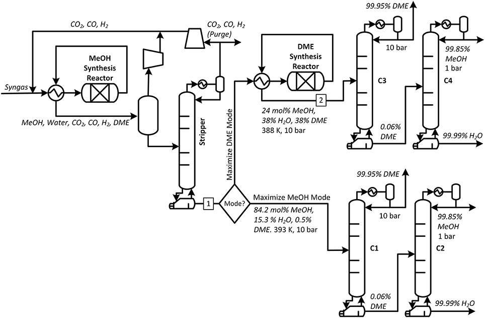
Figure 1. Process overview for the base case design. In this system, syngas is converted to methanol (as well as DME, Water, and gaseous by-products) at steady state and uses a total of four distillation columns. During operation, the system can either be switched into Maximize DME Mode or Maximize Methanol Mode.

Both reactor outputs are first degassed with a flash drum to remove unreacted syngas for recycle/electricity production, and then any gases remaining in the liquid product (mostly CO₂) is removed in a cryogenic distillation column. The bottoms product from the CO₂ removal columns, for both trains, consists of DME, methanol, and water to be separated. The key difference is in content. In this work, we have chosen to use the conditions suggested by Zhang et al. (2010). Under these conditions, the stream leaving the methanol synthesis train (stream 1) contains 84.2 mol% methanol, 15.3 mol% water, and 0.5 mol% DME at 388 K and 10 bar with a total rate of 22,880 kg/h. The corresponding stream leaving the DME synthesis train (stream 284.2) contains 24 mol% methanol, 38% DME, and 38% water at 393 K and 10 bar at the same rate of 22,880 kg/h.

In this study, either the reactor product stream is sent to a conventional distillation sequence (also known as the “direct sequence”) in which DME is recovered in the distillate of the first column and in which the bottoms product is sent to a second column where methanol is removed at the top and water is removed at the bottom¹. Although there are process intensification techniques to perform this three component separation in only one column (such as semicontinuous distillation Pascall and Adams, 2013 or dividing wall distillation Kiss, 2013), we have chosen the classic approach for illustrative purposes. In both trains, the columns are designed to meet the following specifications: the DME product must be chemical grade purity (99.95 mol% Müller and Hübsch, 2000), the methanol product must be chemical grade purity (99.85 mol% Ott et al., 2011), the water product should be 99.99 mol% pure. By mass balance, this means that the bottoms product of the DME removal column should have no more than 0.06 mol% DME in it depending on the mode. The first distillation column in each sequence (C1 and C3) operates at 10 bar while the second column in each sequence (C2 and C4) operates at 1 bar. All columns in the simulation use sieve trays with a tray spacing of 2.0 ft (0.610 m).

Flexible Design A

The alternative flexible polygeneration design is shown in Figure 2. The upstream portions are essentially the same as the Flexible Base Case. The primary difference is that the methanol product and DME product streams (depending on whether the plant is operating in Maximize Methanol Mode or Maximize DME Mode, respectively) are both sent to the same set of distillation columns. The columns must then be designed such that the purity requirements stated in the previous paragraph are met in both Methanol Mode and DME mode. This means that the number of stages above and below the feed, the size of the condenser and reboiler, and the diameter of the column must be chosen such that it is possible to obtain the product purities in either mode only by changing the reflux and reboil ratios in the mode. Essentially, the column must be large enough to both provide the necessary heat duties and prevent flooding in both modes.

FIGURE 2

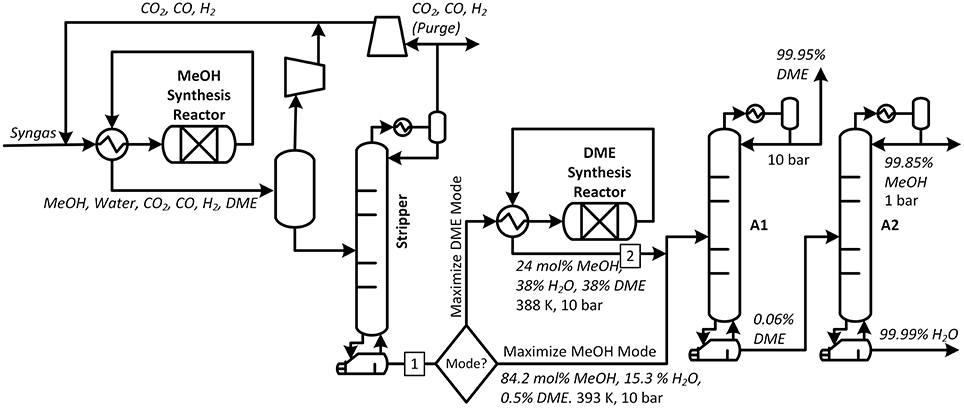
Figure 2. Process overview for Flexible Design A design. In this system, syngas produces methanol (as well as DME, Water, and gaseous by-products) at steady state. During operation, the system can either be switched into Maximize DME Mode or Maximize Methanol Mode, but the same two distillation columns are used in either mode.

Process Simulations

In this study, only the final two distillation columns of each product train are considered for comparison because the upstream unit operations do not differ significantly (or at all) between the Base Case and Flexible Design A. All of the process simulations in this work use the RADFRAC block in Aspen Plus v9.0 in equilibrium mode. Murphree tray efficiencies are set to 85%, which has been shown in other works to be a reasonable number for estimation of sub-equilibrium conditions in similar systems (Tock et al., 2010). The UNIQ-RK method using UNIFAC predicted coefficients for Water + DME binary vapor-liquid equilibria and Aspen Plus default parameters for Water + Methanol and Methanol + DME was used. This method was chosen as the physical property package because we found it to match very well with the ternary experimental vapor-liquid phase equilibria at 9.74 bar and 353 K (Song et al., 2006; close to the feed conditions), with an R² above 0.993. It should be noted that the PRWS method is also an appropriate choice (Pascall and Adams, 2013). For a given number of stages above and below the feed, the Design Spec tool is used to ensure that the product purity specifications are met for each column by varying the reflux and boilup ratios. Of course, when the number of stages above and/or below the feed were too low, product purity constraints could not be met, resulting in an infeasible design. No solution multiplicity was observed. The DISTWU block, which uses shortcut methods for column design, was used to estimate the lower bounds on the total number of column stages and the reflux ratio, as well as generate initial guesses for column parameters and conditions. RADFRAC convergence was aided by a combination of good initial guesses for the internal tray variables (composition, temperature, and flow rates) and occasional manipulation of the convergence algorithm parameters.

Cost Computations

The total annualized cost (TAC) of the DME-Methanol-Water separation section is used in this study as the quality metric for comparison between design choices. Utility costs are computed using $3.36/GJ for refrigeration (needed for the DME product condensers), $0.21/GJ for cooling water (for the methanol product condensers), $2.20/GJ for medium pressure steam (for all reboilers), which were the default values suggested by the Utilities feature in Aspen Plus. It is also assumed that the process operates on-spec for 8,400 h per year. The total direct costs of the distillation columns and heat exchangers are estimated by using fresh-on-board equipment purchase cost curves provided in Turton et al. (2003) multiplied by an installation factor of 2.96. The fresh-on-board cost estimates for the equipment considers factors such as equipment size and dimensions, tray counts, steel thickness, welding efficiency, and maximum allowable stress according to the procedures outlined in that text. The installation factor considers the costs of installation, labor, paint, electrical work, etc., and was determined using an average of various sample cases predicted in Aspen Capital Cost Estimator, noting that it is very close to the corresponding value of the Lang factor suggested in Seider et al. (2008). The Fair method was used in Aspen Plus to compute the column diameters that prevent flooding within a safety factor of 80%, rounded up to the nearest six inch increment. To compute the total surface area of the heat exchangers, an overall heat transfer coefficient of 788 W/(m²-°C) was used, which was the default provided by Aspen Capital Cost Estimator and compares well against values for similar situations in the open literature (Edwards, 2005). All costs in this study are in 2015 US Dollars.

The TAC is computed as a function of the Total Direct Costs (TDC) in dollars and the Annual Operating Cost (AOC) in dollars per year as follows (Smith, 2014):

$\begin{array}{l}TAC=a_{f}TDC+AOC\end{array}$

Where a_f is the annuity factor given by:

$\begin{array}{l}{a}_f=\frac{i{(1+i)}^t}{{(1+i)}^t-1}\end{array}$

Where i is the interest rate per year and t is the total number of years in the lifetime of the plant. For example, for an interest rate of 10% and a lifetime of 15 years, the annuity factor is 0.1314 year⁻¹, which was used in this study. This is roughly equal to using an 8 year lifetime with no interest rate. The annuity rate ultimately determines the weighting between capital and operating costs. For brevity, we only show the results for one annuity factor in this study. A sensitivity analysis was conducted showing that extreme changes in annuity factor affects the design of some columns more than others, but ultimately the same methodology applies for each.

It is assumed that the time required to transition between operating modes (and subsequent off-spec product) is small compared to time spent in on-spec operation since the number of transitions is expected to be relatively small. As such all costs of transitions between operating modes are ignored for this study. Were this information to be included, this would add the additional complexity of needing to estimate the number of transitions expected per year, which would be somewhat arbitrary, and ultimately change the methodology and results very little.

Flexible Polygeneration Optimization Formulation and Solution

Production Expectations

Because of flexible nature of the design, the optimal design for either the Base Case or Case A will depend on how much time the process spends in either Methanol Mode or DME Mode during the lifetime of the facility. For this study, we define two important parameters. First, we define ϕ_Exp,D ∈ [0, 1] to be percentage of the plant's lifetime spent in Maximize DME Mode that we expect during the design phase, prior to the construction of the plant. This number would typically be chosen based on long term predictions of the market, business plans, and other factors. This contrasts with ϕ_Act,D ∈ [0, 1], which is the actual percentage of the time spent in Maximize DME Mode over the course of the plant's entire lifetime. This an uncertain parameter that can only be known at the end of the plant's lifetime because the decision to operate in either mode will change in real time depending on a large number of factors. These factors include market forces such as sale prices, contracts, utility costs, consumer demand, and contracts. However, it also includes other factors such as disaster, plant failures, business goals, and regulations.

Other studies which consider flexible polygeneration under uncertainty use primarily a market-based approach (Chen et al., 2011a; Cheali et al., 2014; Li and Barton, 2015), where the uncertainty in the market prices is considered directly and represented by a probability distribution. This approach is often characterized by having many uncertain market-based parameters which are sampled in some fashion (e.g., through a Monte Carlo method or a scenario-based approach) in order to make design decisions for a process that is intended to last for many decades. Although this formulation can be complex and require novel and advanced techniques to solve, it can result in good designs, and is often a good way to consider factors such as uncertainties in the parameters of the model or process units.

Here, we employ an alternative approach that does not require multiple probability distributions, for which characterization is difficult for typical design horizons of 20–30 years. For example, operating decisions may not in practice be based on optimization of an anticipated performance criterion such as a predefined economic objective, but a reaction to an unanticipated business opportunity or threat. Uncertain factors are consequently combined into the single parameter, ϕ_Act,D, that greatly simplifies the uncertainty characterization and problem formulation, with arguably little or no loss in the adequacy of the design under uncertainty. If desired, the engineer can still use stochastic models, market predictions, price histories, and other such methods to try to predict ϕ_Act,D by determining either a single guess for ϕ_Exp,D (see section Naïve Designs) or a probability distribution function P(ϕ_Exp,D) (see section Formulations for Designs Considering Uncertainty). Other factors such as uncertainty in the model parameters, especially any parameter which is immediately measurable or computed scientifically without forecasting such that distribution functions can be made with high confidence, should still be considered using existing methods such as the one presented by Cheali et al. (2014).

Problem 1 Formulation for Flexible Base Case

Problem Formulation 1 is constructed by assuming that one should find the design with the minimum TAC for a given ϕ_Exp,D without any consideration of uncertainty in the value of ϕ_Act,D. It is a reasonable starting point, because if we had perfect foresight such that ϕ_Exp,D turns out to be exactly equal to ϕ_Act,D, then we will have chosen the absolute best possible design for that plant's lifetime. The minimum TAC for the total system of interest (the four columns C1-C4) is actually the sum total of the minimum TACs for each of the columns independently. This is because each column can be designed completely independently of the others, since feed conditions are fixed to the same conditions for each mode in all cases and the target product specifications are also fixed in all cases. For each individual column, there are only two degrees of freedom: the number of stages above the feed (N_A) and the number of stages below the feed (N_B). For example, in column C1, the feed conditions will always be the same when it is running (in Maximize Methanol Mode), otherwise, it will not be running at all because the system is in DME Mode. Therefore, for any given N_A and N_B for C1, there is only one meaningful set of reflux ratio and boilup ratio pairs that will satisfy the product purity constraints (otherwise, such a column is too short and it is physically impossible to use). However, as long as C1 is feasible, the actual choice of N_A and N_B for C1 has no impact on C2, because reflux and boilup ratio of C1 will always be chosen such that the bottoms product stream will be essentially identical in all cases (except for trivially small differences in DME content). As such, the optimization problem can be formulated as follows:

$\begin{array}{rc}TA{C}_{BaseCase,Exp}={{\displaystyle \sum }}_{c=C1..C4}{Z}_c& (1)\end{array}$

$\begin{array}{rc}{Z}_c={\displaystyle \underset{N_{A,c},N_{B,c}}{min}}TA{C}_{c,Exp}& (2)\end{array}$

$\begin{array}{rc}s.t.TA{C}_{c,Exp}=a_{f}TD{C}_c+AO{C}_{c,Exp}& (3)\end{array}$

$\begin{array}{l}AO{C}_{c,Exp}=h\left(Q_{H,c}{U}_{H,c}+Q_{C,c}{U}_{C,c}\right)\left(1-{\varphi }_{Exp,D}\right)\left(1-{\delta }_c\right)\\ +h\left(Q_{H,c}{U}_{H,c}+Q_{C,c,}{U}_{C,c}\right)\left({\varphi }_{Exp,D}\right){\delta }_c\\ {\delta }_c=\{\begin{array}{ll}0\hfill & forc=C1,C2(MeOHMode)\hfill \\ 1\hfill & forc=C3,C4(DMEmode)\hfill \end{array}& (4)\end{array}$

$\begin{array}{r}TD{C}_c=f_1(A_{C,c})+f_2(A_{H,c})+f_3(N_{A,c}+N_{B,c},D_c)\\ h(x,N_{A,c},N_{B,c})=0\hfill & (5)\end{array}$

$\begin{array}{rc}x=\left[A_{C,c},A_{H,c},D_c,Q_{H,c},Q_{C,c},\dots \right]& (6)\end{array}$

Where c is the column (C1 through C4); Z_c is the minimum TAC of column c; N_A,c and N_B,c are the number of stages above and below the feed for column c, respectively; TDC_c is the total direct cost of column c; TAC_c,Exp and AOE_c,Exp are the expected TAC and AOC of column c respectively; h is the number of hours per year the plant operates on-spec (as defined in section Cost Computations); Q_H,c and Q_C,c are the hourly heat duties of the reboiler and condenser of column c respectively; U_H,c and U_C,cis the cost of utility (per energy basis) of the reboiler and condenser of column c, respectively as given in section Cost Computations; δ_c is a switching parameter that indicates that columns only operate during particular modes; f₁, f₂, and f₃ are polynomial functions for total direct costs of the condenser, reboiler, and column (including trays) for column c, respectively, as described in section Cost Computations; A_C,c and A_H,c are the heat exchanger areas of the condenser and reboiler of column c, respectively; D_c is the diameter of column c; and x is the vector of continuous variables which includes all tray compositions, pressures, temperatures, molar flow rates, reflux and reboil ratio, in addition to the most important variables listed above.

In Problem 1, Equations (3) through (5) are used to compute the total direct costs. Equations (6) are the nonlinear rigorous model equations for distillation column c in RadFrac, including the condenser and reboiler, and also including the constraint equations for the distillate and bottoms purity specifications for column c. These specifications were implemented as design specification within RadFrac. Equation (6) also include the Fair correlation for computing the minimum column diameter necessary to prevent flooding, which is rounded up to nearest six-inch increments to meet typical size standards. As such, (6) is non-smooth. Also, the heat exchanger design equations are included in (6) which relates heat exchanger surface area to the column conditions. There are no explicit inequality equations except for bounds on the continuous variables implicit in the model (for example, mole fractions are between 0 and 1, flow rates are nonnegative, etc.). N_A,c and N_B,c are positive integers, but again, feasible lower bounds can be estimated using shortcut methods such as the DistWU model as a guide.

The above formulation is a non-smooth MINLP, which in general can be difficult to solve. However, for a given instance of N_A,c and N_B,c, Equations (3) through (6) form a square system of equations with respect to the continuous variables which are independent of ϕ_Exp,D. If a feasible solution exists, it can be solved directly (in our case, by converging the Aspen Plus simulation for column c). As such, the problem can be reformulated as follows:

Problem 1

$\begin{array}{rc}TA{C}_{BaseCase,Exp}={{\displaystyle \sum }}_{c=C1..C4}{Z}_c& (7)\end{array}$

$\begin{array}{rc}{Z}_c={\displaystyle \underset{N_{A,c},N_{B,c}}{min}}TA{C}_{c,Exp}& (8)\end{array}$

$\begin{array}{rc}s.t.TA{C}_{c,Exp}=a_{f}TD{C}_c+AO{C}_{c,Exp}& (9)\end{array}$

$\begin{array}{l}AO{C}_{c,Exp}=h(Q_{H,c}{U}_{H,c}+Q_{C,c}{U}_{C,c})\left({1-\varphi }_{Exp,D}\right)(1-{\delta }_c)\\ +h(Q_{H,c}{U}_{H,c}+Q_{C,c,}{U}_{C,c})({\varphi }_{Exp,D}){\delta }_c\hfill & (10)\\ {\delta }_c=\{\begin{array}{l}\mathrm{0 }forc=C1,C2\left(MeOHMode\right)\\ \mathrm{1 }forc=C3,C4\left(DMEmode\right)\end{array}\end{array}$

$\begin{array}{rc}TD{C}_c=f_1(A_{C,c})+f_2(A_{H,c})+f_3(N_{A,c}+N_{B,c},D_c)& (11)\end{array}$

$\begin{array}{rc}{A}_{C,c}=f_{4,c}(N_{A,c},N_{B,c})& (12)\end{array}$

$\begin{array}{rc}{A}_{H,c}=f_{5,c}(N_{A,c},N_{B,c})& (13)\end{array}$

$\begin{array}{rc}{D}_c=f_{6,c}(N_{A,c},N_{B,c})& (14)\end{array}$

$\begin{array}{rc}{Q}_{H,c}=f_{7,c}(N_{A,c},N_{B,c})& (15)\end{array}$

$\begin{array}{rc}{Q}_{C,c}=f_{8,c}(N_{A,c},N_{B,c})& (16)\end{array}$

In Problem 1, the key continuous variables can all be written in explicit form in Equations (12) through (16). The functions f_4,c through f_8,c are dependent on N_A,c and N_B,c only, and are found through exhaustive tabulation for all combinations of N_A,c and N_B,c within the domain of interest. Because there are only two parameters, this can be found relatively quickly by automating a process in which the Aspen Plus simulations are converged for each parameter combination and the pertinent resulting continuous values recorded. For four columns, the total amount of time required to generate this database (approximately 8,000 simulations) is approximately 1 cpu-h, but only needs to be generated one time in total. Once the database has been generated, Problem 1 can be solved in less than a second for any given ϕ_Exp,D by exhaustive search and direct computation of Equations (9) through (11) using a simple MATLAB script, thereby guaranteeing the global optimal solution.

An example result for ϕ_Exp,D = 0.5 is shown in Figure 3. This figure shows expected TAC of each of the four columns as a function of the number of stages above and below the feed of each column. The red square indicates the location of the global optimum. The infeasible region is shown, indicating that the column had too few column sections in order to achieve the product purity constraints—it is a well-known phenomena that any ordinary distillation column requires a certain minimum number of stages to achieve particular purity constraints given certain feed conditions and chemical properties. The area to the upper right of the hypotenuse of the triangle is feasible, but was not explored. In general, for fixed product purity constraints, adding more stages to a distillation column increases capital costs with each stage but yields diminishing returns on condenser and reboiler duty reduction (directly correlated with reflux and boilup ratio). Conversely, as the number of stages decreases, the energy requirement increases, and asymptotically approaches infinity as the number of stages approaches the theoretical minimum. As such, the optimization has only one local minimum within the entire feasible space of N_A,c and N_B,c, and so this local minimum is also the global minimum.

FIGURE 3

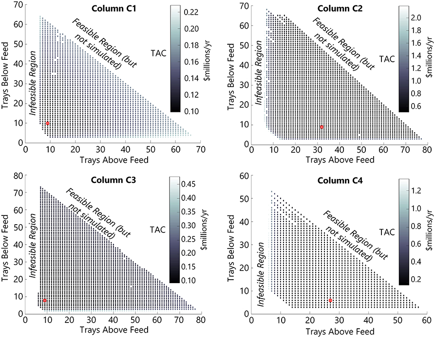
Figure 3. A plot of the expected TAC of each of the four columns (TAC_Exp,C1… TAC_Exp,C4) for the Base Case as a function of N_A,c,N_B,c for ϕ_Exp,D = 0.5. The red square indicates the optimal N_A,c,N_B,c found after solving Problem 1.

Problem 1 was solved on the range of 0 ≤ ϕ_Exp,D ≤ 1 in steps of 0.01, with the results of key parameters shown in Figure 4 as a function of ϕ_Exp,D. Figure 4A shows the optimal expected TAC (shown as the sum total of the TAC of the Methanol Mode and DME Mode sections) is not quite linear as a function of ϕ_Exp,D, but generally monotonically decreasing as the expected percentage of time spent in Maximize DME mode increases. Note that in these plots, there is a sudden drop in the TAC for the ϕ_Exp,D = 0 and ϕ_Exp,D = 1 cases. These are special cases such that if we expect to never actually operate in maximize DME mode (ϕ_Exp,D = 0), we should simply not bother to build the DME Mode section (columns C3 and C4) because it would never be used, and vice versa for ϕ_Exp,D = 1.

FIGURE 4

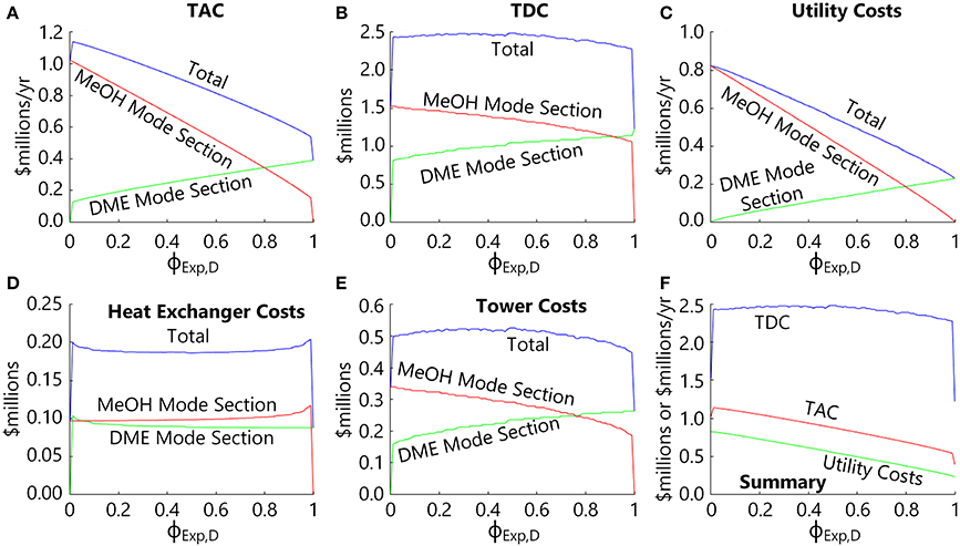
Figure 4. The optimization results of Problem 1 for the Base Case as a function of ϕ_Exp,D). (A) The expected TAC for the Base Case (TAC_BaseCase,Exp), the Methanol Mode section (TAC_C1,Exp + TAC_C2,Exp) and the DME Mode section (TAC_C3,Exp + TAC_C4,Exp). (B) The total direct costs for the Methanol Mode section (TDC_C1 + TDC_C2), the DME Mode section (TDC_C3 + TDC_C4) and their combined total. (C) The expected annual utility costs for the Methanol Mode section (AOC_C1,Exp + AOC_C2,Exp), the DME Mode section (AOC_C3,Exp + AOC_C4,Exp), and their combined total. (D) The heat exchanger capital costs (reboilers and condensers) of the Methanol Mode section (f₁(A_C,C1) + f₁(A_C,C2) + f₂(A_H,C1) + f₂(A_H,C2)), the DME Mode section (f₁(A_C,C3) + f₁(A_C,C4) + f₂(A_H,C3) + f₂(A_H,C4)), and their combined total. (E) The distillation column costs (shell and trays) of the optimal designs of the Methanol Mode section (f₃(N_A,C1, N_B,C1, D_C1) + f₃(N_A,C2,N_B,C2,D_C2)), the DME Mode section (f₃(N_A,C3, N_B,C3,D_C3) + f₃(N_A,C3,N_B,C3,D_C3)), and their combined total. (F) A comparison of the utility, total annualized, and total direct costs of the optimal designs.

Figure 4B shows the total direct costs, which exhibits a small amount of non-smoothness with respect to ϕ_Exp,D. This non-smoothness is not due to the contribution of the heat exchanger capital costs (Figure 4D), but rather the distillation column costs (Figure 4E) which show a distinct non-smoothness with respect to ϕ_Exp,D. This non-smoothness is not due to numerical error (since convergence tolerances are sufficiently tight such that numerical inaccuracy would not appear on the plot) or the finding of a sub-optimal result (since global optimality is guaranteed). Rather, this is due to the discrete nature of the optimization variables N_A,c and N_B,c. For example, as ϕ_Exp,D increases (spending more time in maximize DME mode), it becomes optimal to invest more into the Maximize DME Mode section distillation columns (C3 and C4) by using a greater number of trays in order to save on energy costs, with the opposite effect on the Maximize Methanol Mode section columns (C1 and C2). As shown in (Figure 4E), the costs of C3 + C4 (the DME Mode Section) increases monotonically with ϕ_Exp,D but in a stepwise fashion as trays are added in discrete steps to either C3 or C4, while the costs of C1 + C2 (the Methanol Mode section) decreases monotonically in a similar stepwise fashion. In addition, some of these steps are due to increases in column diameter, which also occurs in discrete six-inch increments. Because the steps are uncorrelated, their sum, the total distillation column cost, either increases or decreases in small steps with respect to ϕ_Exp,D, which results in the “noisy” appearance.

This can be seen more clearly in Figure 5, which shows the individual number of stages in each column independently in Figure 5A, the discrete changes in diameter in Figure 5B, as well as the condenser and reboiler areas. The heat exchanger areas and column diameters change rapidly near ϕ_Exp,D = 0 for the DME Mode columns (C3 and C4) and change rapidly near ϕ_Exp,D = 1 for the Methanol Mode columns (C1 and C2). For example, the condenser area, reboiler area, and minimum diameter necessary to prevent flooding of C2 increases rapidly from 0.9 ≤ ϕ_Exp,D ≤ 1. This is because the number of stages of C2 is relatively small in that region, and so to achieve the same specified product purities with a smaller column, the reflux and reboil ratios must be greatly increased, requiring larger heat exchangers and a wider column to accommodate the larger extra internal column flow rates that results from large reflux ratios.

FIGURE 5

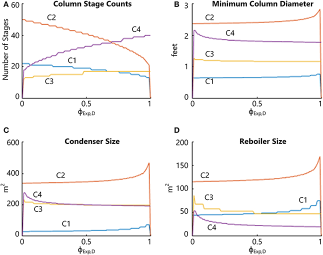
Figure 5. Selected optimal design parameters for the Base Case as a function of ϕ_Exp,D. (A) The number of stages of each distillation column (N_A,c + N_B,c). (B) The minimum diameter of each distillation column before rounding up to the nearest 0.5 ft (0.152 m). increment (D_c). (C) The surface area of the condenser of each distillation column (A_C,c). (D) The same for the reboiler (A_H,c).

Problem 2 Formulation for Flexible Case A—The Integrated Case

For Case A, in which only 2 columns are used, but within different modes of operation, the problem formulation is somewhat different:

Problem 2

$\begin{array}{rc}TA{C}_{CaseA,Exp}={{\displaystyle \sum }}_{c=A1,A2}{Z}_c& (17)\end{array}$

$\begin{array}{rc}{Z}_c={\displaystyle \underset{N_{A,c},N_{B,c}}{min}}TA{C}_{c,Exp}& (18)\end{array}$

$\begin{array}{rc}s.t.TA{C}_{c,Exp}=a_{f}TD{C}_c+AO{C}_{c,Exp}& (19)\end{array}$

$\begin{array}{r}AO{C}_{c,Exp}=h(Q_{H,c,MeOH}{U}_{H,c}+Q_{C,c,MeOH}{U}_{C,c})({1-\varphi }_{Exp,D})\\ +h(Q_{H,c,DME}{U}_{H,c}+Q_{C,c,DME,}{U}_{C,c})({\varphi }_{Exp,D})\hfill & (20)\end{array}$

$\begin{array}{rc}TD{C}_c=f_1(A_{C,c})+f_2(A_{H,c})+f_3(N_{A,c}+N_{B,c},D_c)& (21)\end{array}$

$\begin{array}{ll}{A}_{C,c}=\{\begin{array}{l}\max \left[f_{4,C1}\left(N_{A,c},N_{B,c}\right),f_{4,C3}\left(N_{A,c},N_{B,c}\right)\right] forc=A1\hfill \\ \max \left[f_{4,C2}\left(N_{A,c},N_{B,c}\right),f_{4,C4}\left(N_{A,c},N_{B,c}\right)\right] forc=A2\hfill \end{array}& (22)\end{array}$

$\begin{array}{ll}{A}_{H,c}=\{\begin{array}{l}\max \left[f_{5,C1}\left(N_{A,c},N_{B,c}\right),f_{5,C3}\left(N_{A,c},N_{B,c}\right)\right] forc=A1\\ \max \left[f_{5,C2}\left(N_{A,c},N_{B,c}\right),f_{5,C4}\left(N_{A,c},N_{B,c}\right)\right] forc=A2\end{array}& (23)\end{array}$

$\begin{array}{ll}{D}_c=\{\begin{array}{l}\max \left[f_{6,C1}\left(N_{A,c},N_{B,c}\right),f_{6,C3}\left(N_{A,c},N_{B,c}\right)\right] forc=A1\hfill \\ \max \left[f_{6,C2}\left(N_{A,c},N_{B,c}\right),f_{6,C4}\left(N_{A,c},N_{B,c}\right)\right] forc=A2\hfill \end{array}& (24)\end{array}$

$\begin{array}{ll}{Q}_{H,c,MeOH}=\{\begin{array}{l}{f}_{7,C1}\left(N_{A,c},N_{B,c}\right) forc=A1\hfill \\ f_{7,C2}\left(N_{A,c},N_{B,c}\right) forc=A2\hfill \end{array}& (25)\end{array}$

$\begin{array}{ll}{Q}_{H,c,DME}=\{\begin{array}{l}{f}_{7,C3}\left(N_{A,c},N_{B,c}\right) forc=A1\hfill \\ f_{7,C4}\left(N_{A,c},N_{B,c}\right) forc=A2\hfill \end{array}& (26)\end{array}$

$\begin{array}{ll}{Q}_{C,c,MeOH}=\{\begin{array}{l}{f}_{8,C1}\left(N_{A,c},N_{B,c}\right) forc=A1\hfill \\ f_{8,C2}\left(N_{A,c},N_{B,c}\right) forc=A2\hfill \end{array}& (27)\end{array}$

$\begin{array}{ll}{Q}_{C,c,DME}=\{\begin{array}{l}{f}_{8,C3}\left(N_{A,c},N_{B,c}\right) forc=A1\hfill \\ f_{8,C4}\left(N_{A,c},N_{B,c}\right) forc=A2\hfill \end{array}& (28)\end{array}$

Where Q_H,c,MeOH is the reboiler heat duty of column c when in Maximize Methanol Mode and Q_H,c,DME is the reboiler heat duty of column c when in Maximize DME Mode, with similar definitions for Q_C,c,MeOH and Q_C,c,DME for the condenser. The key differences are that there are now only two columns in Equation (17), so that Equation (20) now reflects that both columns are always on, but in different modes of operation at different times of the year. Equation (22) indicates that during the two different modes of operation, the amount of condenser heat exchanger area actually needed will be different depending on the circumstances, such as the temperature driving force. Therefore, the larger of the two sizes is purchased to ensure that enough heat exchanger area will be available to provide the necessary duty in either case. This is true for both the first (A1) and second (A2) columns. Note that in this equation, f_4,C1 represents the heat exchanger area of the condenser of the first column running in MeOH mode, and f_4,C3 represents the heat exchanger area of the condenser of the first column running in DME mode. In the evaluation of A_C,c, we are able to utilize the tabulated data from the 4-column case considered in Problem 1. Equation (23) indicates a similar concept for the reboiler. Similarly, Equation (24) indicates that the minimum column diameter to prevent flooding may be different in each mode of operation, so that the column should be sized to the larger of the two to ensure that flooding is prevented in each mode. The key advantage of the above formulation is that Equations (22) through (28) use the same database tables as in Problem 1, such that no additional Aspen Plus simulations need to be run. Therefore, Problem 2 can be solved to global optimality in under 1 s for any given ϕ_Exp,D by a simple exhaustive search. Note that the search space is restricted to combinations of N_A,c and N_B,c that will be feasible for both modes of operation. For example, the combination N_A,A1 = 6, N_B,A1 = 14 is not considered because although having 6 stages above the feed and 14 below has a feasible set of operating conditions (condenser and reboiler duties) that meet the design objectives when operating in Methanol mode (see the plot for column C1 in Figure 3), there is no feasible set of operating conditions that will meet the design objectives when operating in DME mode (see plot for column C3 in Figure 3).

The results of the optimization for Flexible Case A as a function of ϕ_Exp,D are shown in Figure 6, with comparisons to the Base Case shown for convenience. Looking at (Figure 6A), it can be seen that the Flexible Case A design has a lower TAC than the Base Case at all ϕ_Exp,D (except for ϕ_Exp,D = 0 or 1, which reduce to the exact same design). The cost savings arises completely from capital cost reduction (Figure 6B) with virtually no savings in energy (Figure 6C). The capital cost savings is due to savings in both the tower costs (Figure 6D) and the heat exchanger costs (Figure 6E), with capital cost savings in the $800,000 to $1 million range (Figure 6F), despite having to oversize all of the equipment to accommodate both Methanol Mode and DME Mode conditions. Thus, this approach has a benefit of about 30–50% capital cost savings with no increase in operating costs.

FIGURE 6

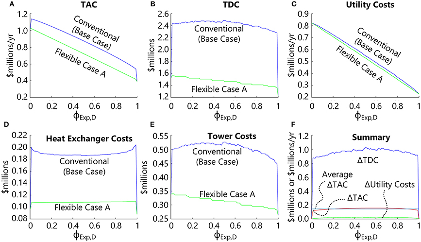
Figure 6. Optimization results for Problem 2 for Flexible Case A as a function of ϕ_Exp,D compared against the optimal Base Case results (see Figure 4). (A) The expected TAC for the Base Case and Case A (TAC_{BaseCase, Exp} and TAC_CaseA,Exp). (B) The total direct costs for the Base Case (TDC_C1 + … + TDC_C4) and Case A (TDC_A1 + TDC_A2). (C) The expected annual utility costs for the Base Case (AOC_C1,Exp + … + AOC_C4,Exp) and for (Case A AOC_A1,Exp + AOC_A2,Exp). (D) The total distillation column costs for the two cases, (E) the total heat exchanger capital costs for the two cases, and (F) the cost difference of the Base Case minus Case A for the utilities (green line), total annualized costs (red line), and total direct costs (blue). The average of the cost difference for TAC (cyan line) is shown to better see the curvature of the red line.

Problem 3 Formulation for Flexible Case B—An Alternative Flexible Design

Although the Case A results are promising, there is another potential area for improvement. The design concept for Case A uses one column (A1) for DME product recovery and the second column (A2) for methanol and water product recovery. However, as shown in Figure 5, the optimal column diameters, stage counts, and heat exchanger sizes can be very different when comparing the same column under the different feed conditions experienced in the Methanol or DME modes. Thus, it may be better in some cases to design a different flexible design with two columns which instead of having one column dedicated to DME product recovery and the other dedicated to Methanol and water recovery, one column is dedicated to the larger job and one is dedicated to the smaller job. This might result in additional capital cost savings because one column would have a large diameter and the other could have a small diameter.

This approach is called Flexible Case B. Here, the products collected in the distillate and bottoms streams of the columns would actually switch depending on the mode of operation, as shown in Figure 7. During Maximize Methanol Mode, the feed is fed to B1 (the “narrow” column) with DME collected in the distillate. The bottoms product is fed to B2 (the “wide” column) where methanol and water are recovered to the desired purities. During Maximize DME Mode, the DME reactor product is sent to B2 instead, with DME collected in the distillate of B2, and the bottoms product sent to B1 to remove methanol and water.

FIGURE 7

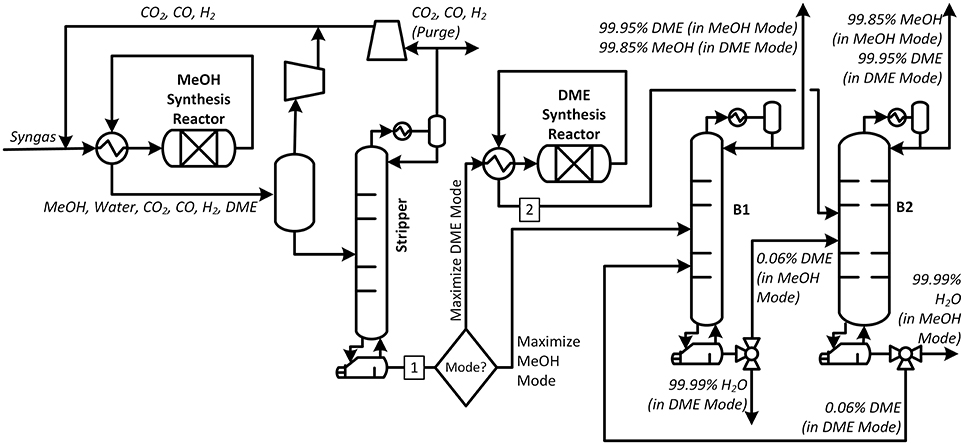
Figure 7. The process for Flexible Case B. The feed is routed to column B1 when in Maximize Methanol Mode and to column B2 when in Maximize DME Mode.

Because of the feed switching manifold, it seems prudent to allow the feed tray to differ at each connection point, since the feed compositions will vary significantly between the two modes. The reboiler and condenser use the same utilities (steam and cooling water, respectively) for both feed modes, although the composition of the stream being serviced will change. The resulting optimal design problem (Problem 3) can be formulated as follows:

Problem 3

$\begin{array}{rc}TA{C}_{CaseB,Exp}={{\displaystyle \sum }}_{c=B1,B2}{Z}_c& (29)\end{array}$

$\begin{array}{rc}{Z}_c={\displaystyle \underset{N_{A,c,MeOH},N_{B,c,MeOH}{,N}_{A,c,DME}}{min}}TA{C}_{c,Exp}& (30)\end{array}$

$\begin{array}{rc}s.t.N_{B,c,DME}=N_{A,c,MeOH}+N_{B,c,MeOH}-N_{A,c,DME}& (31)\end{array}$

$\begin{array}{rc}TA{C}_{c,Exp}=a_{f}TD{C}_c+AO{C}_{c,Exp}& (32)\end{array}$

$\begin{array}{r}AO{C}_{c,Exp}=h(Q_{H,c,MeOH}{U}_{H,c}+Q_{C,c,MeOH}{U}_{C,c})({1-\varphi }_{Exp,D})\\ +h(Q_{H,c,DME}{U}_{H,c}+Q_{C,c,DME,}{U}_{C,c})({\varphi }_{Exp,D})\hfill & (33)\end{array}$

$\begin{array}{rc}TD{C}_c=f_1(A_{C,c})+f_2(A_{H,c})+f_3(N_{A,c,MeOH}+N_{B,c,MeOH},D_c)& (34)\end{array}$

$\begin{array}{ll}{A}_{C,c}=\{\begin{array}{l}\max \left[f_{4,C1}\left(N_{A,c,MeOH},N_{B,c,MeOH}\right),f_{4,C4}\left(N_{A,c,DME},N_{B,c,DME}\right)\right] forc=B1\\ \max \left[f_{4,C2}\left(N_{A,c,MeOH},N_{B,c,MeOH}\right),f_{4,C3}\left(N_{A,c,DME},N_{B,c,DME}\right)\right] forc=B2\end{array}& (35)\end{array}$

$\begin{array}{ll}{A}_{H,c}=\{\begin{array}{l}\max \left[f_{5,C1}\left(N_{A,c,MeOH},N_{B,c,MeOH}\right),f_{5,C4}\left(N_{A,c,DME},N_{B,c,DME}\right)\right] forc=B1\hfill \\ \max \left[f_{5,C2}\left(N_{A,c,MeOH},N_{B,c,MeOH}\right),f_{5,C3}\left(N_{A,c,DME},N_{B,c,DME}\right)\right] forc=B2\hfill \end{array}& (36)\end{array}$

$\begin{array}{ll}{D}_c=\{\begin{array}{l}\max \left[f_{6,C1}\left(N_{A,c,MeOH},N_{B,c,MeOH}\right),f_{6,C4}\left(N_{A,c,DME},N_{B,c,DME}\right)\right] forc=B1\hfill \\ \max \left[f_{6,C2}\left(N_{A,c,MeOH},N_{B,c,MeOH}\right),f_{6,C3}\left(N_{A,c,DME},N_{B,c,DME}\right)\right] forc=B2\hfill \end{array}& (37)\end{array}$

$\begin{array}{ll}{Q}_{H,c,MeOH}=\{\begin{array}{l}{f}_{7,C1}\left(N_{A,c,MeOH},N_{B,c,MeOH}\right) forc=B1\hfill \\ f_{7,C2}\left(N_{A,c,MeOH},N_{B,c,MeOH}\right) forc=B2\hfill \end{array}& (38)\end{array}$

$\begin{array}{ll}{Q}_{H,c,DME}=\{\begin{array}{l}{f}_{7,C4}\left(N_{A,c,DME},N_{B,c,DME}\right) forc=B1\hfill \\ f_{7,C3}\left(N_{A,c,DME},N_{B,c,DME}\right) forc=B2\hfill \end{array}& (39)\end{array}$

$\begin{array}{ll}{Q}_{C,c,MeOH}=\{\begin{array}{l}{f}_{8,C1}\left(N_{A,c,MeOH},N_{B,c,MeOH}\right) forc=B1\hfill \\ f_{8,C2}\left(N_{A,c,MeOH},N_{B,c,MeOH}\right) forc=B2\hfill \end{array}& (40)\end{array}$

$\begin{array}{ll}{Q}_{C,c,DME}=\{\begin{array}{l}{f}_{8,C4}\left(N_{A,c,DME},N_{B,c,DME}\right) forc=B1\hfill \\ f_{8,C3}\left(N_{A,c,DME},N_{B,c,DME}\right) forc=B2\hfill \end{array}& (41)\end{array}$

Problem 3 is similar to Problem 2, except that now there are three integer decision variables for each column: The number of stages above and below the feed when in Maximize Methanol Mode (N_A,c,MeOH and N_B,c,MeOH respectively), and the number of stages above the feed when in Maximize DME Mode (N_A,c,DME). There is a fourth new variable, the number of stages below the feed when in Maximize DME Mode (N_B,c,DME), but this is not independent because the total number of stages of a column in Methanol Mode must be the same as the total number of stages in DME Mode, and is instead calculated explicitly by the constraint in new Equation (31). The remainder of the problem is very similar. Equations (34) through (41) reuse the same functions f₁ through f₈ as tabulated in the previous problems, and do not have to be recomputed again. There are only slight changes in how they are used. For example, in Equation (35), the second term of the maximum functions swaps the calls to f_4,C3 and f_4,C4 to reflect that the columns receiving the primary feed now changes in Case B depending on the mode. Similar swaps are made in Equations (36), (37), (39), and (41). Note that like in Case A, the decision variables are restricted to combinations which result in feasible operation during both modes.

Even though the dimensionality is higher (3 independent variables per minimization problem) the number of individual instances that need to be enumerated is on the order of 50,000, which is still tractable. Since the same data tables can be reused from the previous simulations, Problem 3 can be solved to global optimality for a given ϕ_Exp,D in just a few minutes.

The key results are provided in Figure 8, showing Flexible Case B is actually slightly more expensive than Flexible Case A at any ϕ_Exp,D. Although heat exchanger and utility costs are essentially the same, Flexible Case B requires slightly larger distillation towers on the whole. In this case, Flexible Case A is clearly preferred, not just because of cost, but because transitions between modes are likely to be much easier to do because condenser utilities, feed location, and feed trays do not need to change. However, this result is case specific, and so the approach used in Flexible Case B is still worthy of consideration for other systems of interest. In section Design Under Uncertainty, we have chosen to use Flexible Case B for the design under uncertainty analysis even though it is slightly more expensive than Flexible Case A because Case B has more degrees of freedom and requires more computational power to solve, and therefore better demonstrates that optimal design under uncertainty problems can be solved to guaranteed global optimality using our approach within reasonable amounts of time.

FIGURE 8

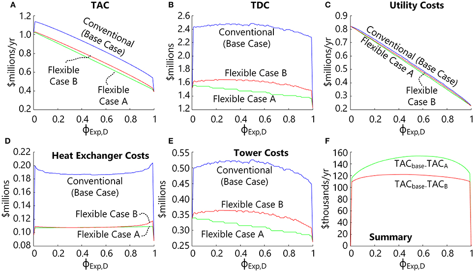
Figure 8. Optimization results for Problem 3 for Flexible Case B as a function of ϕ_Exp,D compared against the Base Case and Case A results (see Figures 4, 6). (A) The expected TAC, (B) the total direct costs, (C) the expected annual utility costs, (D) the total distillation column costs, (E) the total heat exchanger capital costs, and (F) the difference in TAC of the Base Case minus Case A or Case B.

Design Under Uncertainty

Naïve Designs

As demonstrated in section Flexible Polygeneration Optimization Formulation and Solution, the optimal design is a strong function of the expected amount of time spent in Maximize DME Mode over the course of its lifetime. However, this parameter is highly uncertain, and bad predictions can result in a significantly sub-optimal design, as demonstrated in Figure 9. In this figure, 99 Flexible Case B designs were made by solving Problem 3 on the range 0 < ϕ_Exp,D < 1 in steps of 0.01. Then for each of those designs, the actual TAC (TAC_CaseB,Act) was computed as a function of ϕ_Act,D, which is the actual percentage of time spent in Maximize DME mode experienced by the plant once constructed, as follows:

$\begin{array}{r}TA{C}_{CaseB,Act}=a_{f}TD{C}_{B1}+a_{f}TD{C}_{21}+AO{C}_{B1,Act}\\ +AO{C}_{B2,Act}\hfill & (42)\end{array}$

$\begin{array}{r}AO{C}_{c,Act}=h(Q_{H,c,MeOH}{U}_{H,c}+Q_{C,c,MeOH}{U}_{C,c})({1-\varphi }_{Act,D})\\ +h(Q_{H,c,DME}{U}_{H,c}+Q_{C,c,DME,}{U}_{C,c})({\varphi }_{Act,D})\hfill \\ forc=B1,B2\hfill & (43)\end{array}$

Where the Q, U, and a_fTDC_c values are the results from the original Problem 3 solution. As shown in the figure, the best outcome is to predict ϕ_Exp,D exactly, with the minimum TAC_CaseB,Act located along the ϕ_Exp,D = ϕ_Act,D line. For example, suppose after 15 years of use, ϕ_Act,D = 0.2, meaning that the plant operated in DME mode for 20% of its life and operated in Methanol mode for the remaining 80%. Suppose also that the designer of the process had predicted this exactly (in other words, the expected time in DME mode was 20%, or ϕ_Exp,D = 0.2), and chose to build the design that resulted from Problem 3 using ϕ_Exp,D = 0.2. The total actual TAC experienced over 15 years in this case (Point A in Figure 9) is about $0.928 million TAC/year, as shown in Figure 9. This is also the true global optimal design for the outcome/realization of ϕ_Act,D = 0.2, since there are no other designs that could have achieved a lower TAC for this outcome.

FIGURE 9

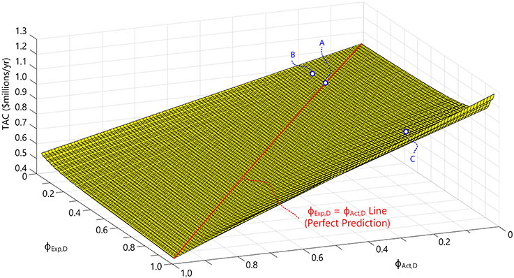
Figure 9. The actual TAC for Flexible Case B (TAC_CaseB,Act) as a function of the expected time spent in DME mode (ϕ_Exp,D) and the actual time spent in DME mode (ϕ_Act,D) if designed naïvely without consideration of uncertainty.

However, suppose that after 15 years of use, ϕ_Act,D = 0.2, but the designer had expected that the system would run in DME mode only 10% of the time, and so had chosen to build the design that resulted from solving Problem 3 using ϕ_Exp,D = 0.1 (point B in Figure 9). This is a suboptimal result, because the actual TAC experienced in this case is a little higher at $0.929 million TAC/year. The further ϕ_Exp,D deviates from ϕ_Act,D, the worse the prediction, and the higher the actual TAC goes. For example, suppose the prediction turned out to be very bad at ϕ_Exp,D = 0.8 since the actual time spent in DME mode was only 20% (point C in Figure 9). The actual TAC after 15 years in this case is much higher at $0.984 million TAC/year.

Formulations for Designs Considering Uncertainty

Uncertainty can be considered by slightly reformulating the objective function to minimize the expected costs considering a probability distribution instead of a single value of ϕ_Exp,D, as follows:

$\begin{array}{l}TA{C}_{CaseB,Exp}={{\displaystyle \sum }}_{c=B1,B2}{Z}_c\\ Z_c={\displaystyle \underset{N_{A,c,MeOH},N_{B,c,MeOH}{N}_{A,c,DME}}{min}}& (44)\end{array}$

$\begin{array}{rc}{\displaystyle {\int }_0^1}P({\varphi }_{Exp,D})TA{C}_{c,Exp}({\varphi }_{Exp,D})d{\varphi }_{Exp,D}& (45)\end{array}$

subject to the same Equations (31) through (41) above, where P(ϕ_Exp,D) is the probability distribution function such that ${\int }_0^{1}P({\varphi }_{Exp,D})d{\varphi }_{Exp,D}=1$ and all probabilities P are specified and P(ϕ_Exp,D) ≥ 0. In practice, the integral is intractable to compute analytically and so it is instead approximated numerically as a collection of discrete scenarios of possible ϕ_Exp,D. This change results in Problem 4 as shown:

Problem 4

$\begin{array}{l}TA{C}_{CaseB,Exp}={{\displaystyle \sum }}_{c=B1,B2}{Z}_c\\ Z_c={\displaystyle \underset{N_{A,c,MeOH},N_{B,c,MeOH}{N}_{A,c,DME}}{min}}& (46)\end{array}$

$\begin{array}{rc}{{\displaystyle \sum }}_{i=1}^{i=S}P({\varphi }_{Exp,D,i})TA{C}_{c,Exp,i}({\varphi }_{Exp,D,i})& (47)\end{array}$

$\begin{array}{rc}s.t.TA{C}_{c,Exp,i}=a_{f}TD{C}_c+AO{C}_{c,Exp,i}& (48)\end{array}$

$\begin{array}{r}AO{C}_{c,Exp,i}=h(Q_{H,c,MeOH}{U}_{H,c}+Q_{C,c,MeOH}{U}_{C,c})({1-\varphi }_{Exp,D,i})\\ +h(Q_{H,c,DME}{U}_{H,c}+Q_{C,c,DME,}{U}_{C,c})({\varphi }_{Exp,D,i})\hfill & (49)\end{array}$

plus Equations (31, 34) through (41) above, where ϕ_Exp,D,i is the expected time spent in DME Mode for scenario i, S is the number of scenarios considered, and $\sum _{i=1}^{i=S}P({\varphi }_{Exp,D,i})=1$ where all probabilities P are specified and P(ϕ_Exp,D,i) ≥ 0. The expected TAC and AOC must be enumerated by scenario, but otherwise the remainder of the equations are the same. Again, this problem makes use of the same database tables, and so no additional simulations need to be performed and the global optimal solution can again be found feasibly by enumeration. Problem 4 reduces to Problem 3 for a single scenario (S = 1). Problem 4 required about 17 cpu-s to solve for S = 99 per instance of the distribution function. However, Problem 4 is also embarrassingly parallel (except for overhead) in the individual scenarios (since they can be computed in parallel), as well as the individual instances of the three decision variables when solving by enumeration.

A second, robust formulation can be also made which does not require any guessing of the probability distribution at all. This is useful to generate a worst-case estimate of the optimal design, such that the optimal design chosen is the one that has the cheapest worst-case TAC for any distribution of the Methanol / DME Modes. This results in Problem 5:

Problem 5

$\begin{array}{ll}TA{C}_{CaseB,Exp}={{\displaystyle \sum }}_{c=B1,B2}{Z}_c& (50)\end{array}$

$\begin{array}{ll}\begin{array}{c}{Z}_c=\underset{N_{A,c,MeOH}, N_{B,c,MeOH}{N}_{A,c,DME}}{\min }\underset{i=\mathrm{1..}s}{\max }TA{C}_{c,Exp,i}({\varphi }_{Exp,D,i})\end{array}& (51)\end{array}$

Subject to all of the constraints of Problem 4: Equations (31), (34) through (41), (48), and (49).

Problem 5 requires essentially the same computation time as Problem 4 and can be solved to guaranteed global optimality.

Comparison of Designs Under Uncertainty

Problem 4 was solved for a uniform distribution function with S = 99 evenly-spaced scenarios of equal probability ranging from 0 < ϕ_Exp,D,i < 1 and compared to the results of Problem 5 with the same scenario distribution. Both approaches can be used to select a single design without any prior knowledge of its final use. S = 99 was chosen as the result of starting with lower resolutions (i.e., S = 9) and increasing the resolution until the results no longer changed. The final design resulting from the solution of Problem 4 uses B1 with 22 stages with a diameter of 2 ft. (0.610 m) and B2 with 51 stages and a diameter of 2.5 ft (0.762 m). The Problem 5 result was a little bit different, with B1 having 33 stages at 2 ft. (0.610 m) diameter and B2 having 41 stages at 2.5 ft (0.762 m) diameter. Figure 10 shows the TAC of those two designs as a function of ϕ_Act,D. The results show that both approaches are comparable, since either one or the other results in lower actual TAC depending on the actual amount of time spent in each mode over its lifetime (ϕ_Act,D), but both give similar performance in all cases anyway. However, both are preferable to the naïve approach used in Problem 3. For example, when comparing to Figure 9, although guessing ϕ_Exp,D,i = ϕ_Act,D exactly correct during the design phase results in the lowest TAC possible (or the “true” optimum), these two design under uncertainty approaches which require no a piori knowledge of the market at all are not very far from the “true” optimum. In fact, the uniform distribution result at ϕ_Act,D = 0.5 is exactly the same as the true optimum design for ϕ_Act,D = 0.5, and the robust min-max formulation result at ϕ_Act,D = 0.5 has only 4.3% higher TAC than the true optimum for ϕ_Act,D = 0.5. Both methods avoid bad results when bad guesses for ϕ_Exp,D,i are used in the naïve approach.

FIGURE 10

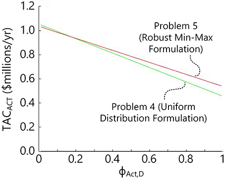
Figure 10. The actual TAC of Flexible Case B when designed by solving Problem 4 with a uniform probability distribution and by solving Problem 5 (the robust min-max formulation), as a function of ϕ_Act,D.

In addition, we performed a sensitivity analysis on Problem 5 by varying the annuity factor, with results shown in the Supplementary Material. The design of column B1 changed little over the range, but B2 changed more significantly (larger columns were favored with lower annuity factor).

Although the robust approach can be used to prevent extreme circumstances, having good predictive knowledge of the future market can lead to cost savings. Problem 4 was re-run repeatedly using a normal distribution centered around different mean expected percentage of time spent in DME Mode (${\overline{\varphi }}_{Exp,D}$) with a standard deviation of σ = 0.5 (absolute). The distributions were truncated on the range 0 < ϕ_Exp,D < 1 and normalized such that $\sum _{i=1}^{i=S}P({\varphi }_{Exp,D,i})=1$. Each different distribution examined used 99 scenarios. This represents the case that we have good predictions of the expected ϕ_Exp,D but with a reasonable amount of uncertainty. The results are shown in Figure 11, with the Figure 9 results shown again for ease of comparison.

FIGURE 11

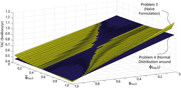
Figure 11. The actual TAC as a function of the mean expected ${\overline{\varphi }}_{Exp,D}$ of the prediction and the actual ϕ_Act,D using the Problem 4 formulation, with the results from the naïve approach from Figure 9 included.

The results confirm that when the guesses for ${\overline{\varphi }}_{Exp,D}$ are accurate, it is better to use the naïve approach (the yellow surface), noting that it has lower TAC just below the blue hourglass-shaped region that runs axial to the ${\overline{\varphi }}_{Exp,D}={\varphi }_{Act,D}$ line. This is easiest to see in the bottom corner of Figure 11 at the point (${\overline{\varphi }}_{Exp,D}=1$, ϕ_Act,D = 1), where the yellow surface is just slightly below the blue surface. However, the more inaccurate the predicted ${\overline{\varphi }}_{Exp,D}$ is, the better the design under uncertainty approach with a normal distribution will be since it will have the lower TAC. This is easiest to see on the left and right corners of Figure 11 [the points (${\overline{\varphi }}_{Exp,D}=0$, ϕ_Act,D = 1) and (${\overline{\varphi }}_{Exp,D}=1$, ϕ_Act,D = 0), respectively], where the blue surface is the below the yellow surface by a relatively large amount. Therefore, the key advantage of the design under uncertainty approach is that large penalties from very bad guesses are avoided, and yet when guesses are good, there is only a slight penalty for “over design” compared to the naïve approach. Thus, on the whole, the design under uncertainty approach better manages the risk.

Although not shown in Figure 11 for brevity, Problem 4 was repeated several times using a normal distribution function with different assumed standard deviations in uncertainty. As σ increased, the results converged toward the uniform distribution solution, and as σ decreased, the results converged toward the naïve solution. This is interesting because in practice, even with good long-term predictive models, σ is itself uncertain. In this example, this means that it is probably not worth the expense of creating good long-term predictive models to predict ${\overline{\varphi }}_{Exp,D}$ with high confidence (small σ), because the uniform distribution approach provides results that are nearly as good when predictions are accurate and yet the savings achieved by avoiding large penalties when predictions are bad (even if unlikely) are quite large. Although this might not be true for some other systems, the methodology presented in this work can be used to make those assessments rather quickly because of the problem formulation and solution strategy.

In addition, we note that only issues related to market uncertainty were addressed in this work, but other kinds of uncertainties, were not. Depending on the type uncertainty considered, the above methods can be adapted in various ways. For example, resolving Problems 3–5 using different annuity factors or utility costs (or scenario-based probability functions of them) requires relatively little additional computational effort because none of the tabulated functions f ₁ through f ₉ need to be recomputed. When changing capital cost estimates, only f ₁ through f ₃ need to be retabulated or rewritten as continuous functions, which is relatively fast since the simulations do not need to be rerun. However, considering uncertainty in the model itself may require repeated re-simulation of the distillation columns, for which our approach may not be suitable.

Conclusions

This study presented two flexible versions of a distillation process designed to handle large changes in feed composition in order to produce different chemical products based on market demand. The study addressed the question of how to best design the process by using a design under uncertainty approach, since the market conditions that the plant will experience over its long lifetime are highly uncertain. In this work, we demonstrated a methodology which breaks down an otherwise complex problem into discrete, rigorously modeled subproblems that allows us to find global optimal solutions quickly, which is summarized in Figure 12. In this way, different design under uncertainty approaches could be directly and fairly compared with a minimum number of assumptions.

FIGURE 12

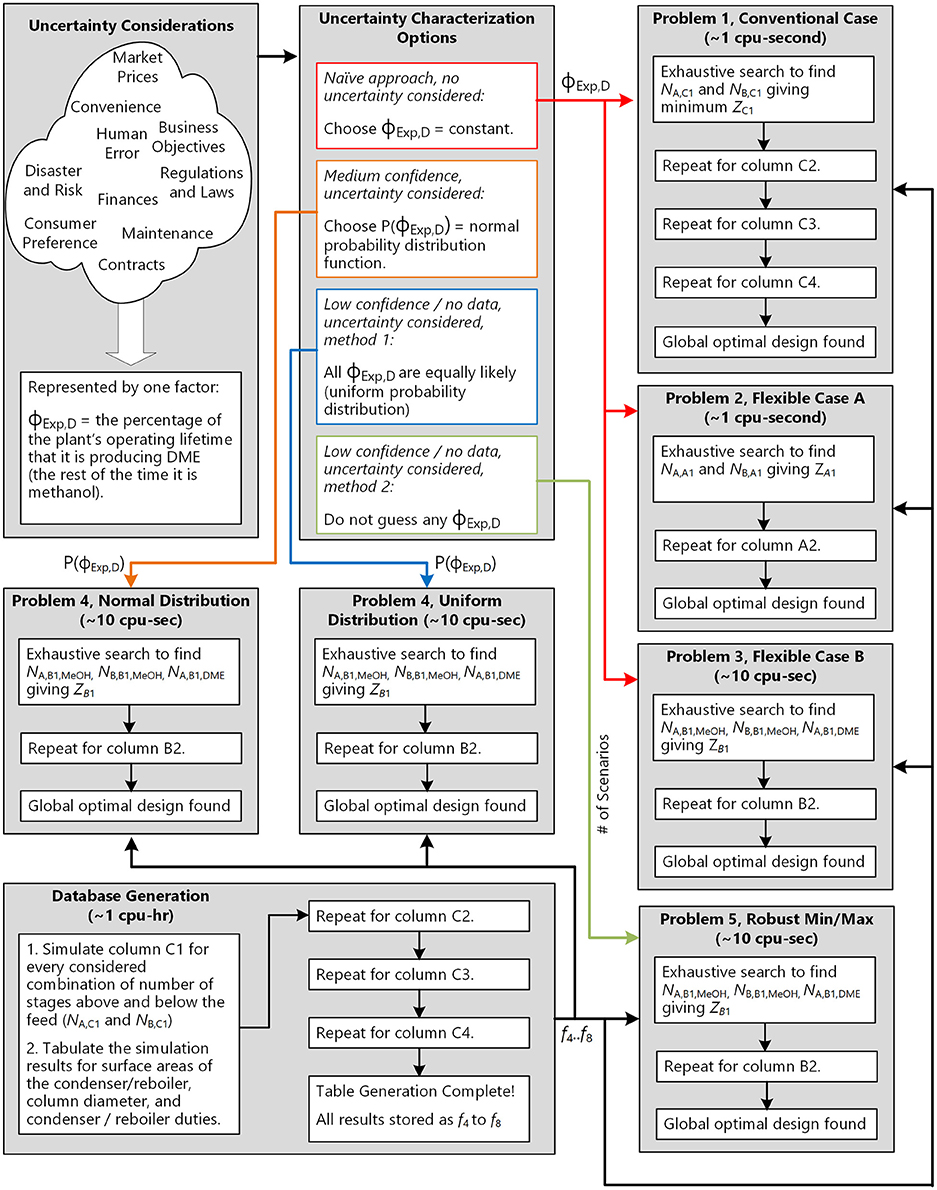
Figure 12. A summary of the methodology used in this work. Essentially, the results of the single database generation step can be re-used in a variety of different problem formulations based on the design concept and the market uncertainty characterization.

The study found that using two “over-designed” distillation columns capable of achieving product purities under both feed scenario required between 30 and 40% lower total depreciable capital than using four distillation columns which were specifically tailored to best suit each feed scenario. The operating costs, however, were approximately the same. The optimal choice of which specific design was best was strongly related to the expected market conditions during the lifetime of the plant, which is highly uncertain. The results showed that using a design under uncertainty uniform distribution function or using a robust min-max approach both resulted in very good individual designs that performed well no matter how often one mode was used versus the other. The results also showed that choosing a process based on guesses (even considering uncertainty) for the percentage of time that each mode would actually be used in practice resulted in only slight gains when the guesses were accurate but large losses where the guesses were inaccurate. Therefore, the uniform distribution approach was recommended as the best design methodology for this scenario.

Although the results are interesting for the uncertain Methanol/DME market switching scenario, the methodology and optimization framework presented herein is useful for many other applications because it makes it possible to consider very large optimal design problems of this type under uncertainty in a very reasonable amount of CPU-time without loss of fidelity. For distillation trains in general, this approach could be used for any number of ordinary binary distillation columns in series in which their sequence was already known. Special configurations such as dividing wall columns and Petlyuk configurations may add more complexity but the general framework could still be used. Because our design approach decouples each column from the other, the computation time of the solution to the optimal design problem under uncertainty scales linearly with the number of distillation columns in sequence and linearly with the number of uncertainty scenarios considered. The solution algorithm is in theory almost embarrassingly parallel, although that was not experimentally verified in this work.

In addition, the methodology presented decouples the most computationally demanding portions of the optimization problem (rigorous tray-by-tray distillation column models in Aspen Plus) from the rest of the optimization, such that the results of the process simulations can tabulated off-line. Once tabulated, the optimal design problems under uncertainty can be solved extremely quickly because all important continuous variables can be computed explicitly via table lookup or a trivially simple calculation, and the same lookup tables can be re-used for a great many different optimization problems. Thus, the methodology makes it possible to solve each problem to global optimality via brute-force enumeration of the decision variables in a short amount of time.

Author Contributions

TA directed research and wrote the paper. TT and ML performed research. CS directed research and contributed to paper writing.

Funding

Funding for this work was provided by Ontario Research Fund–Research Excellence grant 05-072 and the McMaster Advanced Control Consortium.

Conflict of Interest Statement

The authors declare that the research was conducted in the absence of any commercial or financial relationships that could be construed as a potential conflict of interest.

Supplementary Material

The Supplementary Material for this article can be found online at: https://www.frontiersin.org/articles/10.3389/fenrg.2018.00041/full#supplementary-material

Abbreviations

AOC, annual operating cost; DME, dimethyl ether; NPV, net present value; TAC, total annualized cost; TDC, total direct costs; a_f, annuity factor; A_H,c, heat exchanger area of the reboiler of column c; A_C,c, heat exchanger area of the condenser of column c; AOE_c,Exp, expected annual operating cost for column c; c, subset variable, index for column number; D_c, diameter of column c; f, a function in the model, implemented either as set of equations or a lookup table; h, number of hours per year the plant operates on-spec; i, interest rate; N_A,c, number of stages above the feed for column c (does not change with mode); N_A,c,DME, number of stages above the feed for column c when in Maximize DME Mode; N_A,c,MeOH, number of stages above the feed for column c when in Maximize Methanol Mode; N_B,c, number of stages below the feed for column c (does not change with mode); N_B,c,DME, number of stages below the feed for column c when in Maximize DME Mode; N_B,c,MeOH, number of stages below the feed for column c when in Maximize Methanol Mode; P, a probability function or distribution; Q_H,c, heating duty for column c (does not change with mode); Q_H,c,DME, heating duty for column c when operating in Maximize DME Mode; Q_H,c,MeOH, heating duty for column c when operating in Maximize Methanol Mode; Q_C,c, cooling duty for column c (does not change with mode); Q_C,c,DME, cooling duty for column c when operating in Maximize DME Mode; Q_C,c,MeOH, cooling duty for column c when operating in Maximize Methanol Mode; S, number of scenarios considered; t, total plant lifetime (years); TAC_c,Exp, expected total annualized cost for column c; TAC_{CaseB, Act}, the actual TAC of the system of Case B over the plant's lifetime; TDC_c, total direct cost of column c; U_H,c, utility price for heating for column c ($/GJ); U_C,c, utility price for cooling for column c ($/GJ); x, vector of continuous variables in the model; Z_c, minimum TAC of column c; δ_c, switching parameter (binary) indicating that column c operates in a particular mode; σ, standard deviation of a normal probability distribution; ϕ_Exp,D, the percentage of the plant's lifetime that we expect to operate in Maximize DME Mode; ϕ_Exp,D, ϕ_Exp,D but specifically for scenario i; ϕ_Exp,D, the mean expected value in a normal probability distribution P(ϕ_Exp,D); ϕ_Act,D, the percentage of the plant's lifetime that actually operated in Maximize DME Mode.

Footnotes

1. ^It is likely in practice that in Maximize DME mode, the methanol recovered would be recycled to the DME synthesis reactor, but this is not considered in this study.

References

Adams, T. A. II., and Ghouse, J. H. (2015). Polygeneration of fuels and chemicals. Curr. Opin. Chem. Eng. 10, 87–93. doi: 10.1016/j.coche.2015.09.006

CrossRef Full Text | Google Scholar

An, W., Chuang, K. T., and Sanger, A. R. (2004). Dehydration of methanol to dimethyl ether by catalytic distillation. Can. J. Chem. Eng. 82, 948–955. doi: 10.1002/cjce.5450820510

CrossRef Full Text | Google Scholar

Birge, J. R., and Louveau, F. (1997). Introduction to Stochastic Programming. New York, NY: Springer-Verlag.

Google Scholar

Burger, L., and Schwarz, C. E. (2018). Sensitivity of process design to phase equilibrium uncertainty: study of isopropyl + DIPE + 2-methoxyethanol system. Fluid Phase Equilib 458, 234–242. doi: 10.1016/j.fluid.2017.11.027

CrossRef Full Text | Google Scholar

Chakraborty, A., and Linninger, A. A. (2003). Plant-wide waste management. 2. Decision making under uncertainty. Ind. Eng. Chem. Res. 42, 357–369. doi: 10.1021/ie020340o

CrossRef Full Text | Google Scholar

Cheali, P., Quaglia, A., Gernaey, K., and Sin, G. (2014). Effect of market price uncertainties on the design of optimal biorefinery systems – A systematic approach. Ind. Eng. Chem. Res. 53, 6021–6032. doi: 10.1021/ie4042164

CrossRef Full Text | Google Scholar

Chen, Y., Adams, T. A. II., and Barton, P. I. (2011b). Optimal design and operation of static energy polygeneration systems. Ind. Chem. Eng. Res. 50, 5099–5113. doi: 10.1021/ie101568v

CrossRef Full Text | Google Scholar

Chen, Y., Adams, T. A. II., and Barton, P. I. (2011a). Optimal design and operation of flexible energy polygeneration systems. Ind. Chem. Eng. Res. 59, 4553–4566. doi: 10.1021/ie1021267

CrossRef Full Text | Google Scholar

Chen, Y., Li, X., Adams, T. A. II., and Barton, P. I. (2012). Decomposition strategy for the global optimization of flexible energy polygeneration systems. AIChE J. 58, 3080–3095. doi: 10.1002/aic.13708

CrossRef Full Text | Google Scholar

Dimitriadis, V. D., and Pistikopoulos, E. N. (1995). Flexibility analysis of dynamic systems. Ind. Eng. Chem. Res. 34, 4451–4462. doi: 10.1021/ie00039a036

CrossRef Full Text | Google Scholar

Edwards, J. E. (2005). Design and Rating Shell-and-Tube Heat Exchangers. P I Des. Ltd, Teesside.

Grossmann, I. E., and Floudas, C. A. (1987). Active constraint strategy for flexibility analysis of chemical processes. Comp. Chem. Eng. 11, 675–693. doi: 10.1016/0098-1354(87)87011-4

CrossRef Full Text | Google Scholar

Grossmann, I. E., Apap, R. M., Calfa, B. A., Garcia-Herreros, P., and Zhang, Q. (2016). Recent advances in mathematical programming techniques for the optimization of process systems under uncertainty. Comp. Chem. Eng. 91, 3–14. doi: 10.1016/j.compchemeng.2016.03.002

CrossRef Full Text | Google Scholar

Grossmann, I. R., Calfa, B. A., and Garcia-Herreros, P. (2014). Evolution of concepts and models for quantifying resiliency and flexibility of chemical processes. Comp. Chem. Eng. 70, 22–34. doi: 10.1016/j.compchemeng.2013.12.013

CrossRef Full Text | Google Scholar

Gupta, A., and Maranas, C. D. (2003). Managing demand uncertainty in supply chain planning. Comp. Chem. Eng. 27, 1219–1227. doi: 10.1016/S0098-1354(03)00048-6

CrossRef Full Text | Google Scholar

Halemane, K. P., and Grossmann, I. E. (1983). Optimal process design under uncertainty. AIChE J. 29, 425–433. doi: 10.1002/aic.690290312

CrossRef Full Text | Google Scholar

Kiss, A. A., and Suszwalak, D. J. P. C. (2012). Innovative dimethyl ether synthesis in a reactive dividing-wall column. Comp. Chem. Eng. 38, 74–81. doi: 10.1016/j.compchemeng.2011.11.012

CrossRef Full Text | Google Scholar

Kiss, A. A. (2013). Novel applications of dividing-wall column technology to biofuel production processes. J. Chem. Technol. Biotechnol. 88, 1387–1404. doi: 10.1002/jctb.4108

CrossRef Full Text | Google Scholar

Li, X., and Barton, P. I. (2015). Optimal design and operation of energy systems under uncertainty. J. Proc. Cont. 30, 1–9. doi: 10.1016/j.jprocont.2014.11.004

CrossRef Full Text | Google Scholar

Liu, P., Pistikopoulos, E. N., and Li, Z. (2010). Decomposition based stochastic programming approach for polygeneration energy system design under uncertainty. Ind. Eng. Chem. Res. 49, 3295–3305. doi: 10.1021/ie901490g

CrossRef Full Text | Google Scholar

Müller, M., and Hübsch, U. (2000). “Dimethyl Ether,” Ullmann's Encyclopedia of Industrial Chemistry. Weinheim: Wiley-VCH Verlag GmbH & Co. KGaA.

Mastragostino, R., and Swartz, C. L. E. (2014). Dynamic operability analysis of process supply chains for forest industry transformation. Ind. Eng. Chem. Res. 53, 9825–9840. doi: 10.1021/ie500608w

CrossRef Full Text | Google Scholar

Ogawa, T., Inoue, N., Shikada, T., and Ohno, T. (2003). Direct dimethyl ether synthesis. J. Nat. Gas. Chem. 12, 219–227.

Google Scholar

Ott, J., Gronemann, V., Pontzen, F., Fiedler, E., Grossmann, G., Kersebohm, D. B., et al. (2011). “Methanol,” Ullmann's Encyclopedia of Industrial Chemistry, Vol 3. Weinheim: Wiley-VCH Verlag GmbH & Co. KGaA.

Pascall, A., and Adams, T. A. I. I. (2013). Semicontinuous separation of dimethyl ether (DME) produced from biomass. Can. J. Chem. Eng. 91, 1003–1021. doi: 10.1002/cjce.21813

CrossRef Full Text | Google Scholar

Rooney, W. C., and Biegler, L. T. (1999). Incorporating joint confidence regions into design under uncertainty. Comp. Chem. Eng. 23, 1563–1575. doi: 10.1016/S0098-1354(99)00311-7

CrossRef Full Text | Google Scholar

Seider, W. D., Seader, J. D., Lewin, D. R., and Widago, S. (2008). Product and Process Design Principles: Synthesis, Analysis and Design, 3rd Edn. Hoboken, NJ: Wiley.

Sirdeshpande, A. R., Ierapetritou, M. G., Andrecovich, M. J., and Naumovitz, J. P. (2005). Process synthesis optimization and flexibility evaluation of air separation cycles. AIChE J. 51, 1190–1200. doi: 10.1002/aic.10377

CrossRef Full Text | Google Scholar

Smith, R. (2014). Chemical Process Design and Integration. West Sussex: Wiley.

Google Scholar

Song, H., Zhang, H., Ying, W., and Fang, D. (2006). Measurement and calculation of vapor-liquid equilibrium for dimethyl ether-methanol-water ternary system. J. Chem. Ind. Eng. China 57, 1871–1876.

Swaney, R. E., and Grossmann, I. E. (1985). An index for operational flexibility in chemical process design. Part I: Formulation and theory. AIChE J. 31, 621–630. doi: 10.1002/aic.690310412

CrossRef Full Text | Google Scholar

Tock, L., Gassner, M., and Maréchal, F. (2010). Thermochemical production of liquid fuels from biomass: thermo-economic modeling, process design and process integration analysis. Biomass Bioenergy 34, 1838–1854. doi: 10.1016/j.biombioe.2010.07.018

CrossRef Full Text | Google Scholar

Tsiakis, P., Shah, N., and Pantelides, C. C. (2001). Design of multi-echelon supply chain networks under demand uncertainty. Ind. Eng. Chem. Res. 40, 3585–3604. doi: 10.1021/ie0100030

CrossRef Full Text | Google Scholar

Turton, R., Bailie, R. C., Whiting, W. B., and Shaeiwitz, J. A. (2003). Analysis, Synthesis and Design of Chemical Processes, 2nd Edn. Upper Saddle River, NJ: Prentice Hall.

Google Scholar

Wang, H., Mastragostino, R., and Swartz, C. L. E. (2016). Flexibility analysis of process supply chain networks. Comp. Chem. Eng. 84, 409–421. doi: 10.1016/j.compchemeng.2015.07.016

CrossRef Full Text | Google Scholar

Whiting, W. B. (1996). Effects of uncertainties in thermodynamic data models and models on process calculations. J. Chem. Eng. Data 41, 935–941. doi: 10.1021/je9600764

CrossRef Full Text | Google Scholar

Xu, M., Lunsford, J. H., Goodman, D. W., and Bhattacharyya, A. (1997). Synthesis of dimethyl ether (DME) from methanol over solid-acid catalysts. Appl. Catal. A Gen. 149, 289–301. doi: 10.1016/S0926-860X(96)00275-X

CrossRef Full Text | Google Scholar

Zhang, J., Liang, S., and Feng, X. (2010). A novel multi-effect methanol distillation process. Chem. Eng. Proces. 49, 1031–1037. doi: 10.1016/j.cep.2010.07.003

CrossRef Full Text | Google Scholar

Zhu, Y., Legg, S., and Laird, C. D. (2010). Optimal design of cryogenic air separation columns under uncertainty. Comp. Chem. Eng. 34, 1377–1384. doi: 10.1016/j.compchemeng.2010.02.007

CrossRef Full Text | Google Scholar