A Multi-Criteria Decision Analysis Approach to Facility Siting in a Wood-Based Depot-and-Biorefinery Supply Chain Model

Introduction

Annual feedstock supply variability and significant upfront capital costs can affect investor willingness to commit funds for the construction and operation of cellulosic and advanced biorefineries (Coyle, 2010). To mitigate supply risk in regions of low biomass availability, depots have been found useful for procuring and preprocessing feedstock (Hansen et al., 2015; Lamers et al., 2015a,b). Capital construction cost savings may be found through repurposing existing facilities into a biorefinery when the infrastructure and equipment are compatible with the biorefinery design (Martinkus and Wolcott, 2017). Additionally, operational cost savings may be gained through the selective siting of depots and biorefineries based on location-specific costs such as energy rates and delivered feedstock cost (Martinkus et al., 2017b). Prioritizing capital and operational cost savings during site selection can enable biorefineries and depots to be constructed with reduced financial risk.

Potential biorefinery locations are often selected based solely on general location characteristics (e.g., population, proximity to rail, etc.) with the assumption that a greenfield site can be found within the geographic boundaries (Panichelli and Gnansounou, 2008; Parker et al., 2008; Stephen et al., 2010; Zhang et al., 2011; Ng and Maravelias, 2016). Others assume every pixel, grid point, or county centroid is a potential biorefinery location in a study region or along a roadway (Graham et al., 2000; Noon et al., 2002; Wilson, 2009; Kocoloski et al., 2011; You et al., 2012; Lewis et al., 2014). Still others (Ma et al., 2005; Sultana and Kumar, 2012) expand on the pixel approach by performing an exclusion analysis using rasterized layers to identify potential biomass-based facilities. These approaches may be adequate when performing a scoping analysis for biorefinery siting as they broadly assume a suitable location can be found within the pixels or region identified as optimal. However, a strategic siting analysis should focus on reducing capital and operational biorefinery costs to lessen the barrier to entry into the fuels marketplace. Research has found that location characteristics and economic determinants influence site selection (Kenkel and Holcomb, 2006; Stewart and Lambert, 2011; Fortenbery et al., 2013). Therefore, strategic siting decisions must include considerations for location-specific cost variables to reduce capital and operational expenses.

A centralized, or integrated, biorefinery includes all biomass processing units from preprocessing through conversion into fuel, while in a distributed biorefinery, some of the initial processes occur at a separate location, such as a depot. The integrated biorefinery's feedstock collection area is the immediate radius surrounding the biorefinery, whereas depots can draw biomass from geographically separate locations and marginal lands previously inaccessible (Argo et al., 2013). The technical feasibility of depots in a biorefinery supply chain model has been explored in depth by others for preprocessing and pretreating cellulosic material to reduce the biorefinery footprint and operational costs (Carolan et al., 2007; Eranki et al., 2011; Bals and Dale, 2012; Argo et al., 2013; Hansen et al., 2015; Kim and Dale, 2015; Lamers et al., 2015a,b). All of these studies assume the biorefineries and depots would be greenfield facilities. Ng and Maravelias (2016) assume depots could co-locate with farms for biomass drying and densification, yet they do not provide siting criteria for farm selection. All facilities these studies are sited in optimized locations based on minimizing transportation and feedstock costs without considering other facility expenses that may impart additional influence on the overall cost to procure and process feedstock.

A multi-criteria decision analysis (MCDA) approach can be useful for facility siting analyses that utilize disparate siting criteria. The most-often used MCDA tool in biorefinery siting is the Analytic Hierarchy Process (Saaty, 2008; Sultana and Kumar, 2012; Van Dael et al., 2012). Stakeholders perform pairwise comparisons between all criteria in a siting analysis to determine the relative importance of each criterion, from which criteria weights are derived. Individual facilities or sites are then scored based on their location-specific criteria multiplied by the respective criteria weights. While this method provides a quantitative facility scoring method, the criterion weights are inherently biased due to the relative criteria importance determined qualitatively by the stakeholders.

Perimenis et al. (2011) developed an MCDA tool using a modified version of the AHP to aid users in selecting biofuel production pathways from multiple feedstock and conversion pathways. Production pathway criteria included qualitative and quantitative measures, and a pairwise comparison was performed by the researchers to determine the criteria weights. The range of values for each criterion was translated into a given grade scale. Production pathway scores were developed by multiplying criterion scaled values by their respective criterion weight.

Martinkus et al. (2017b) built on this approach by using economic and social metrics in a facility siting decision support tool (DST) to assess existing industrial facilities for their potential role as a repurposed biorefinery. Operational cost components that vary geospatially (such as feedstock cost or energy rates) were selected as the economic siting criteria. The range of values for the siting criteria in each metric were translated into a grade scale to assess the list of existing facilities within the region for their compatibility with the “biorefinery design case.” Economic siting criteria weights were developed through assessing the biorefinery techno-economic analysis (TEA) to determine the annual percentage cost of each geospatial operational cost out of the total geospatial operational costs. This approach to weight derivation removes inherent biases that may be present in pairwise comparisons. Existing facilities were scored based on how well their individual site characteristics compared to the biorefinery design case.

The aim of this research is to develop a methodology for assessing existing facilities for their potential role in a distributed supply chain for biomass processing and biofuel creation. The objectives are to (1) select existing facilities to serve as depots for a given potential biorefinery through considering location-specific operational costs, and (2) identify the depot-and-biorefinery configuration that provides the least processing and transportation costs from an array of potential depot and biorefinery locations for a given end user.

Researchers have studied the benefits of repurposing facilities into biorefineries, applied MCDA to biorefinery site selection, and utilized depots in biorefinery supply chain analysis, but none to our knowledge have combined all three approaches into one siting model. The MCDA approach utilized in this work is presented as a decision matrix developed to assess industrial facilities and primary biomass processing facilities for their potential inclusion in a biofuel supply chain. Coupled with a transportation cost model, supply chains are developed, and the supply chain that procures and processes biomass into biofuel at the least-cost for a given end user can then be identified. A case study is presented in the Inland Northwest region of the United States, and the results are compared against an optimization routine to determine how well facilities are selected by the decision support tool.

Methodology

Facility siting for both the depots and biorefinery is comprised of a series of steps (Figure 1) that center around two multi-criteria decision matrices, one for the assignment of depots to each potential biorefinery and one for the selection of a final biorefinery location based on the depots + biorefinery configuration. The following sections describe the general form of the decision matrix, a general overview of the depot-and-biorefinery site selection process, and the general form of the Total Transportation Cost Model that is used to develop delivered feedstock costs.

FIGURE 1

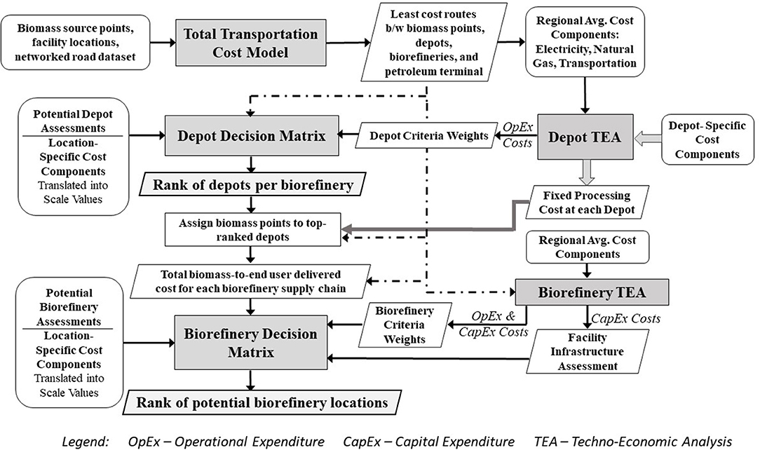
Figure 1. Process flow diagram for depot-and-biorefinery facility siting model.

Generalized Form of Decision Matrix

The decision matrix presented here (Table 1) is based on work by Martinkus et al. (2017b). The decision matrix defines facility siting criteria, weights, and scale values. Criteria are selected as geospatial metrics important in the siting of a biorefinery or depot, weights define the relative importance of each criterion, and scale values provide a means for assessing existing facilities against the design biorefinery case based on location-specific values relative to the range of regional values present.

TABLE 1

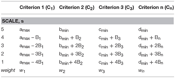
Table 1. Generalized form of the decision matrix.

The rationale behind using geospatial cost components as siting criteria stems from the knowledge that costs for feedstock, energy, and labor vary between locales. The infrastructure present at each facility also varies by facility. The decision matrix allows candidate facilities to be assessed based on their assets or rates in relation to the range of regional values for each cost component. Here, the scale values, s, range from 1 to 5. A “5” indicates a facility rate or asset that provides the least cost for a criterion component, and a “1” indicates an asset that may add significant additional cost to the construction or operation of a facility.

An average annual cost is determined for each geospatial cost component, c_i, through inputting regional average rates into the TEA and aggregating the total amount spent from all operational units in the facility. For example, a regional average electricity rate is input into the TEA, and the total annual amount of electricity used is summed over all units that require electricity. Weights, w_i, are determined by calculating each cost component's percentage of the total annual cost of all geospatial cost components used as siting criteria (n) (Equation 1). The maximum scale value in the decision matrix, s_max, is used to normalize the weights. Each facility j's score, F_j, is calculated by multiplying each weight by the location-specific scale value, s_ji, for each siting criterion using the Weighted Sum Method (Wang et al., 2009) (Equation 2).

$\begin{array}{rc}{w}_i=\left(\frac{c_i}{{\displaystyle {\sum }_{i=1}^n}{c}_i}\right)*\frac{100}{s_{max}}& (1)\end{array}$

$\begin{array}{rc}{F}_j={\displaystyle \sum _{i=1}^n}{w}_i*s_{ji}& (2)\end{array}$

Each criterion's range of regional values is used to determine its scale value designation in the decision matrix. These criterion “bin” values (B_i) are determined by dividing the range of regional values (a_{i, max}, a_{i, min}) by the maximum scale value (s_max) for each criterion i (Equation 3). For each criterion, the maximum scale value is assigned to the minimum or maximum range value that denotes the most positive influence on facility siting, such as high infrastructure repurpose potential or low electricity rate (Martinkus et al., 2017b). The subsequent scale values are calculated by either adding or subtracting B_i, depending on the positive or negative influence of the criterion (Table 1) (Martinkus et al., 2017b). Where regional values are not available or possible, as in infrastructure assessments or delivered feedstock cost, bin values are determined from the range of facility values (Martinkus et al., 2017b).

$\begin{array}{rc}{B}_i=\frac{a_{i,max}-a_{i,min}}{S_{max}}& (3)\end{array}$

General Overview of Depot and Biorefinery Site Selection Process

Potential depot and biorefinery locations are first identified in a region of interest based on their compatibility with the biorefinery feedstock and proximity to other facilities. For example, in a wood-based biofuel supply chain, potential depots are identified as active sawmills and potential biorefineries are identified as active or recently decommissioned pulp mills, since all are compatible with woody feedstock. All facilities are then assessed to ensure their site acreage is sufficient for the design depot and biorefinery footprints as well as for storing a percentage of the annual feedstock demand.

A Total Transportation Cost Model (TTCM) is used to determine the least-cost routes between biomass (feedstock) sources, depots, biorefineries, and the end user. The model is developed in a geographic information system (GIS) platform, and includes a networked road dataset with a cost per road segment for each truck type that will haul the biomass in its various forms along the supply chain. Point locations (or nodes) are added to represent the biomass sources, depots, biorefineries, and the end user. Results from the model include a total cost to transport the material along the shortest distance between each node of the supply chain.

Facility siting criteria selection and weight derivations for both the biorefinery and depot decision matrices are performed using their respective TEAs. Depot siting criteria are derived from the operational expenditures (OpEx) that vary geospatially, such as feedstock, energy, and labor. From the TTCM, a weighted average delivered feedstock cost is determined for each depot at a set annual feedstock demand. To develop criteria weights, the average of all depot weighted average delivered feedstock costs is determined and input into the depot TEA as the feedstock cost, along with regional average energy rates. The annual expense for each criterion is determined, and the percentage of each expense out of the sum of all geospatial expenses is calculated (Equation 1). These percentages are normalized and represent the criteria weights for use in the decision matrix.

One depot decision matrix is developed for each potential biorefinery to identify the top-ranking depots that will contribute biomass to the biorefinery most efficiently. Each potential depot is assessed using the depot decision matrix, and a scale value is assigned for each criterion in the matrix based on the depot's location-specific value relative to the range of values used to define the criterion. Each criterion scale value is multiplied by the respective criterion weight, and the numbers are summed to develop the facility score (Equation 2). The facilities are ranked from highest to lowest score, with the highest-ranking depots having lower energy, feedstock, and labor costs as compared to the range of potential locations assessed. The number of depots selected to provide preprocessed feedstock to a biorefinery is dependent on the size (i.e., feedstock demand) of the design depot modeled in the TEA and the annual feedstock demand of the biorefinery.

If top-ranking depots are located in close proximity to one another, only one will be chosen and the next-ranked depot on the list will be selected. This removes biomass competition between proximal facilities that would force feedstock costs higher. Each depot's delivered feedstock cost is initially determined without consideration for biomass competition from other depots. Once the final depots are selected for inclusion in a biorefinery supply chain, biomass source nodes must be assigned to each of the final depots to determine their final weighted average delivered feedstock cost. This can be performed using an optimization model.

A total cost for each depot-and-biorefinery supply chain is developed by first summing each selected depot's biomass processing cost with the cost to transport densified biomass to the biorefinery, then averaging the resulting costs, and finally, summing with the cost to transport biofuel to the end user. Each depot's processing cost is determined by inputting the depot-specific delivered feedstock cost and energy/labor rates into the TEA and calculating the minimum selling price of the densified feedstock.

The depot-and-biorefinery supply chain total cost is used as a siting criterion in the biorefinery decision matrix, along with other geospatial operational siting criteria identified in the biorefinery TEA, such as energy and labor. An additional siting criterion is included for assessing facility repurpose potential, as we assume that capital expenditure (CapEx) cost savings may be gained through repurposing an existing facility as opposed to constructing a greenfield biorefinery. Biorefinery siting criteria and weights are derived similarly as for the depot decision matrix, and the depot-and-biorefinery supply chains are assessed and scored similarly as well. The top-ranked depot-and-biorefinery supply chain procures, processes, and transports material at the least-cost for the region of interest. It must be noted that in this analysis depots are considered to be co-located with an existing facility, and the depot decision matrix may include a siting criterion to reflect facility repurpose potential if needed.

Total Transportation Cost Model, TTCM

The TTCM determines the delivered feedstock cost and volume between two nodes along the supply chain using a multiple-origin, multiple destination algorithm based on Dijkstra's algorithm for finding the shortest path between two points (Dijkstra, 1959; Esri, 2015). Nodes are locations of biomass procurement or processing, and linkages are the road or rail network that connect nodes.

A networked road dataset is utilized in a GIS environment, and includes a transport cost for each road or rail segment used in the analysis. The general form of the TTCM between two nodes for road or rail transport is represented in Equation (4) (Sultana and Kumar, 2012; Martinkus et al., 2017a).

$\begin{array}{rc}T{C}_{bj}=F_b+V_{bj}& (4)\end{array}$

where TC_bj is the total delivered feedstock cost between nodes b and j, F_b is the fixed cost associated with node b, and V_bj is the total variable transport cost for the least-cost route between nodes b and j. Each road segment is assigned a cost per unit of biomass based on the road type, truck type, biomass moisture content and density, and speed limit of the assumed truck type on the given road type. Variable cost is distance- and/or-time dependent, therefore V_bj is represented by an equation to solve for the cost along each road segment. Equation (5) represents the generic form of a variable cost equation, where 2*V_x is the roundtrip transport cost for road segment x, and n is the total number of road segments in the least-cost path between nodes b and j. If rail transport is used, V_x is not doubled as we assume there is no backhaul.

$\begin{array}{rc}{V}_{bj}=2{\displaystyle \sum _{x=1}^n}{V}_x& (5)\end{array}$

Equation (6) represents the weighted average delivered feedstock cost, WA_j, to a given depot j at a set facility design capacity (Sultana and Kumar, 2012).

$\begin{array}{rc}W{A}_j=\frac{\left({\displaystyle {\sum }_{i=1}^y}T{C}_{bj}{B}_b\right)}{B_j}& (6)\end{array}$

where TC_bj is the total delivered feedstock cost of biomass source point b to depot j, B_b is the biomass volume at source point b, y is the total number of biomass source points supplying depot j to meet facility demand, and B_j is the total volume of feedstock delivered to depot j (i.e., facility demand). Where rail and road are compared along a linkage, the minimum of the two transport methods is selected to provide the least-cost route along the supply chain.

Case Study

The depot-and-biorefinery siting model is applied in the Inland Northwest region of the United States, including western Montana, the panhandle of Idaho, and eastern Washington (Figure 2). Forest residues as a by-product of logging operations are assessed as a feedstock for the creation of isoparaffinic kerosene, or aviation biofuel. In this region where the Federal Government is the major landholder, forest residue is generated in significantly less quantities than regions where forests are primarily privately owned and where the climate is wetter (Martinkus et al., 2017a). Therefore, depots are proposed in this region to preprocess/pretreat residue.

FIGURE 2

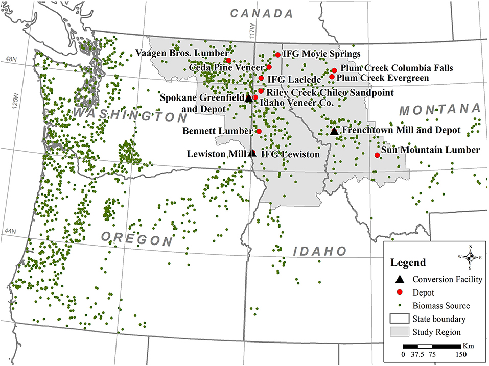
Figure 2. Biomass source nodes and potential biorefinery and depot locations.

The depots are modeled here using a three-stage dry-milling process to create micronized wood particles (~30 microns) as a means of pretreatment (Wang et al., 2018). This process is utilized as no chemicals are necessary to break down the crystalline microstructure of lignocellulose, thus producing a clean sugar with no potential for causing catalyst poisoning or enzyme inhibitors (Brandt et al., 2018). Additionally, water is not needed, which lowers the environmental impact and the need for a wastewater treatment plant at the depot.

The depots must collectively meet an annual biorefinery demand of 300,000 bone dry metric tons (BDMT), accounting for 9% losses through the depots. We assume one large depot with an annual demand of 180,000 BDMT is co-located at the biorefinery to capitalize on nearby biomass, while two smaller satellite depots each procure 60,000 BDMT of forest residue annually. The biorefinery will create ~11.3 million liters of aviation biofuel per year using an enzymatic hydrolysis, fermentation, and separation process (Gao and Neogi, 2015; Hawkins and Ley, 2016). The biofuel will supplement the Spokane, WA regional annual jet fuel demand with ~20% of their year 2025 demand (Macfarlane et al., 2011; Federal Aviation Administration, 2016). A petroleum terminal located near the town's airport and military base is assumed to receive, blend, and store the fuel.

Biorefinery site requirements include a minimum lot size of 40.5 ha, access to natural gas, and a rail spur. Three facilities are evaluated as potential biorefineries: a decommissioned pulp mill in Frenchtown, MT; an active kraft pulp mill in Lewiston, ID; and, a greenfield site in Spokane, WA. The greenfield site is included to assess the hypothesis that repurposed facilities provide significant capital cost savings over greenfields. Primary wood processors (e.g., sawmills and plywood mills) are considered as potential depot locations. Satellite depot siting considerations include access to natural gas, at least 5 ha of unused land for depot site development, and a rail spur. Additionally, where multiple mills reside in the same town or in close proximity, one representative mill is selected for analysis. Of the 27 primary processors in the region, 11 meet the siting requirements. The IFG Lewiston saw mill is co-located with the Lewiston pulp mill, therefore it acts as the large co-located depot as well as a potential satellite depot in this analysis. A large theoretical depot is assumed at the Spokane greenfield and at the Frenchtown Mill for co-location with the biorefineries (Figure 2).

Total Transportation Cost Model, TTCM

U.S. Forest Service Forest Inventory and Analysis (FIA) plots represent biomass source nodes (United States Forest Service, 2016). The Land Use Resource Allocation (LURA) bioeconomic model determines the projected 20-year average annual forest residue volume available at each FIA plot based on future timber market influences (Martinkus et al., 2017a; Latta et al., 2018). Similar to Chung and Anderson (2012), each FIA point is assumed to be a forest landing and is projected onto the nearest road for use in the TTCM. Each road segment is assigned a variable cost based on the material being hauled and associated truck type. Fixed and variable cost calculations for the three supply chain linkages are discussed below. See Martinkus et al. (2017a) for more detail on supply curve development.

Biomass Source-to-Depot

Based on work by Zamora-Cristales et al. (2013) and Martinkus et al. (2017a), a 6x4 chip van truck pulling a 13.7 m (45 ft) long drop center trailer is assumed for wood chip transport. The wood chips are assumed to have a moisture content of 35%, which translates into a payload of 14.1 BDMT. Fixed costs include transporting unmerchantable residue to a forest landing ($16.5/BDMT), grinding the residue into chips ($22.4/BDMT), and loading the chips onto a waiting chip van ($3.9/ BDMT). The speed limit of the networked road dataset was modified based on average chip van speed and tractor-trailer weight loaded and unloaded on paved (70 km/h), gravel (15 km/h), and dirt (10 km/h) roads (Zamora-Cristales et al., 2013). The roundtrip variable unit trucking cost for each road type is based on known truck operating costs when loaded and unloaded (Zamora-Cristales et al., 2013; Martinkus et al., 2017a) (Equation 7).

$\begin{array}{rc}T{C}_{bj}=47.2+0.258{\displaystyle \sum _{p=1}^n}{t}_p+0.194{\displaystyle \sum _{g=1}^n}{t}_g+0.184{\displaystyle \sum _{d=1}^n}{t}_d& (7)\end{array}$

where TC_bj is the total delivered feedstock cost ($/BDMT) along a least-cost route between FIA point b and depot j, t_p is the travel time (min) along all paved road segments, t_g is the travel time (min) along all gravel road segments, t_d is the travel time (min) along all dirt road segments, and n is the total number of road segments by type in the route.

Depot-to-Biorefinery

A 30,280 liter liquid tanker truck is assumed for transporting micronized wood to the biorefinery. This truck type was selected as a sealed vessel is needed to transport the wood particles and it must be pneumatically loaded and unloaded. Micronized wood has a moisture content of 10% and bulk density of 585 kg/m³ (Wang et al., 2018) which translates to a payload of 16.3 BDMT. The road network was modified with speeds representative of this truck type (interstate-−96.5 km/h, U.S. highways-−80.5 km/h, and local roads, state, and county highways-−48 km/h). Fixed and variable transportation costs are derived from Parker et al. (2008), with liquid truck capacity converted to dry capacity (Equation 8). The fixed cost represents loading and unloading wait time.

$\begin{array}{rc}T{C}_{jk,t}=8.54+2\left[1.98{\displaystyle \sum _{t=1}^n}{x}_t+0.05{\displaystyle \sum _{d=1}^n}{x}_d\right]& (8)\end{array}$

where TC_{jk, t} is the total delivered feedstock cost ($/BDMT) between depot j and biorefinery k using truck transport, x_t is the travel time (hrs) along road segment x, x_d is the distance (km) along road segment x, and n is the total number of road segments in the least-cost route.

Rail transport was also assessed for this linkage using an equation derived from Parker et al. (2008). A 124,740 liter rail tanker is assumed to haul the micronized wood with a payload of the 80.5 BDMT. The fixed cost includes loading, unloading, and a charge for use of the railcar (Equation 9).

$\begin{array}{rc}T{C}_{jk,r}=50.13+0.023{\displaystyle \sum _{r=1}^n}{y}_r& (9)\end{array}$

where TC_{jk, r} is the total delivered feedstock cost ($/BDMT) between depot j and biorefinery k using rail transport, y_r is the distance (km) along rail segment y, and n is the total number of rail segments in the least-cost route.

Biorefinery-to-Petroleum Terminal

The same rail and truck tanker types are assumed to transport aviation biofuel to the petroleum terminal in Spokane, WA. Therefore, the equations are the same with unit costs modified based on biofuel volume (Equations 10, 11).

$\begin{array}{rc}T{C}_{kl,t}=0.56+2\left[0.10{\displaystyle \sum _{t=1}^n}{x}_t+0.003{\displaystyle \sum _{d=1}^n}{x}_d\right]& (10)\end{array}$

$\begin{array}{rc}T{C}_{kl,r}=2.92+0.001{\displaystyle \sum _{r=1}^n}{y}_r& (11)\end{array}$

where TC_{kl, t} ($/BDMT) and TC_{kl, r} ($/BDMT) are the total delivered feedstock cost between biorefinery k and petroleum terminal l for truck and rail, respectively, x_t is the travel time (hrs) along road segment x, x_d is the distance (km) along road segment x, y_r is the distance (km) along rail segment y, and n is the total number of road or rail segments in the least-cost route.

Satellite Depot TEA and Decision Matrix

Table 2 lists the operational cost components as identified in the satellite depot TEA, which was developed through modifying Brandt et al. (2018)'s TEA based on depot size and regional energy rates. The Brandt et al. (2018) TEA may be viewed in that manuscript's Supplemental Information. The first four cost components vary geospatially, thus are the siting criteria in the depot decision matrix. The resulting annual geospatial operational costs are converted into percentages of the total cost and then into weights (Table 2, Equation 1). TEA inputs include average county-level energy data (2011-2015) (U.S. Energy Information Administration, 2014a,b), weekly labor rates (2012-2015) (U.S. Bureau of Labor Statistics, 2015), and the average of all weighted average delivered feedstock costs for 60,000 BDMT of forest residue to each potential satellite depot.

TABLE 2

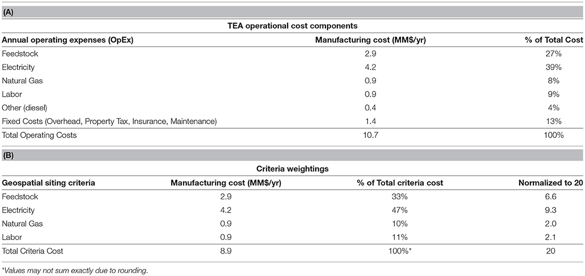
Table 2. (A) Satellite depot operational costs and (B) conversion into decision matrix weights.

Each criterion's range of regional or depot-specific values is additionally used to determine the depot decision matrix bin values (Equation 3) for use in facility assessments. The region is defined as all counties from which biomass is utilized in the supply chain or a potential depot resides (Figure 2). The feedstock criterion is measured as the weighted average delivered feedstock cost, WA_j, for 60,000 BDMT of forest residue to depot j plus the transportation cost to deliver micronized wood from depot j to biorefinery k, TC_jk (Equation 12). One depot decision matrix is created for each potential biorefinery, since the transportation cost from the depots to each biorefinery changes based on biorefinery location. Table 3 shows the decision matrix used to assess all potential depots for the Spokane biorefinery supply chain. See the Supplemental Information (SI) for the Lewiston and Frenchtown depot decision matrices, associated potential depot scaled values and final scores, and breakdown of transportation costs between biomass source points-to-depots, and depots-to-biorefineries.

$\begin{array}{rc}T{C}_{bk}=W{A}_j+T{C}_{jk}& (12)\end{array}$

While the regional weighted average delivered feedstock cost is used in the TEA, the “feedstock” criterion here gives preference to those facilities that are efficient at procuring biomass, processing it into micronized wood and transporting preprocessed material to a biorefinery. Depot-specific criterion values (Table 4) are translated into scale values based on their position relative to the range of regional values (Table 5). Facility scores are determined using Equation (2), and are ranked from greatest to least (Table 6). Facilities with the highest scores would operate at lesser annual operational costs than those with lower scores.

TABLE 3

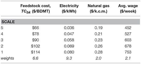
Table 3. Satellite depot decision matrix for spokane biorefinery.

TABLE 4

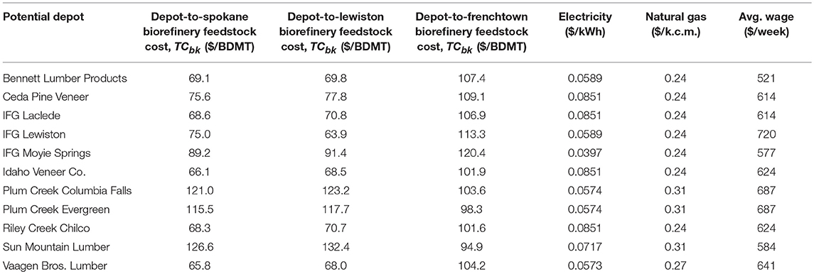
Table 4. Location-specific criterion values for each potential depot.

TABLE 5

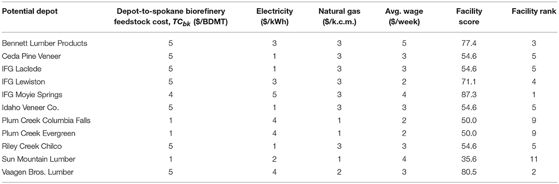
Table 5. Potential depot scaled values for spokane biorefinery supply chain.

TABLE 6

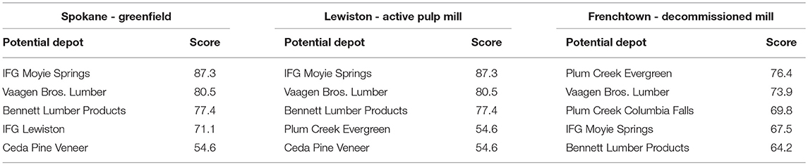
Table 6. Top 5 depot facility scores per biorefinery.

The top two depots for both the Spokane, WA and Lewiston, ID biorefineries are IFG Moyie Springs and Vaagen Brothers Lumber, and the top depots for Frenchtown, MT are Plum Creek Evergreen and Vaagen Brothers Lumber. IFG Moyie Springs was selected as a depot for both Spokane and Lewiston because of its significantly lower electricity cost as compared to all other locations, and Vaagen Brothers Lumber was selected as a depot for all three cases because of the low feedstock transportation and lower electricity costs. Even though feedstock transportation costs are higher, Vaagen Brothers Lumber was selected as a depot for Frenchtown because of its lower electricity and natural gas costs as compared to other locations. Further details are provided in the Supplemental Information.

After the initial depot ranks are completed, an optimization model is then used to assign biomass source points to each of the top two satellite depots and biorefinery co-located depot to meet the overall biorefinery demand of 300,000 BDMT based on minimizing the total delivered feedstock cost from each biomass source point to the biorefinery gate (Figure 3).

FIGURE 3

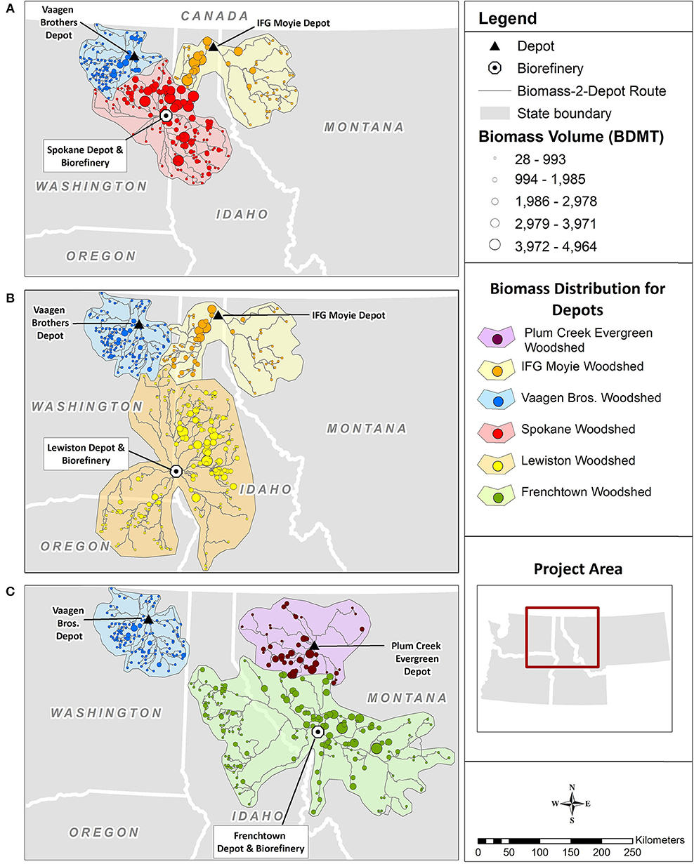
Figure 3. Biomass source point distribution and depot “woodshed” service areas for the (A) Spokane, (B) Lewiston, and (C) Frenchtown biorefinery.

Biorefinery TEA and Decision Matrix

The biorefinery TEA used in this analysis is a modified version a TEA developed by Marrs et al. (2016) for a large integrated biorefinery (757,500 BDMT/year of feedstock) that creates aviation biofuel using a mild bisulfite solution to pretreat wood chips. The major changes to the original TEA include removal of the chemical pretreatment technology to reflect pretreatment occurring at depots, and scaling each department to the smaller biorefinery size used in this analysis.

In addition to energy, labor, and feedstock as biorefinery siting criteria, the infrastructure present at each potential biorefinery is included as a siting criterion (Table 7). This criterion is quantified as the estimated percent reduction in capital construction costs from a greenfield biorefinery through repurposing an existing facility. Percent reductions are determined using a method presented by Martinkus and Wolcott (2017), where a factored analysis is used to estimate cost savings through similarities in infrastructure and assets to a greenfield biorefinery. The total delivered equipment cost for all major processing components in a greenfield biorefinery are required, and all other ancillary assets and infrastructure are estimated as percentages of the total delivered equipment cost. A yes/no analysis is employed for all facilities assessed, where equipment cost is assigned to those components in the assessed facility that are not similar to the greenfield, and no cost is assigned to equipment that is present. All costs are summed to determine the estimated percent savings over constructing a greenfield biorefinery.

TABLE 7

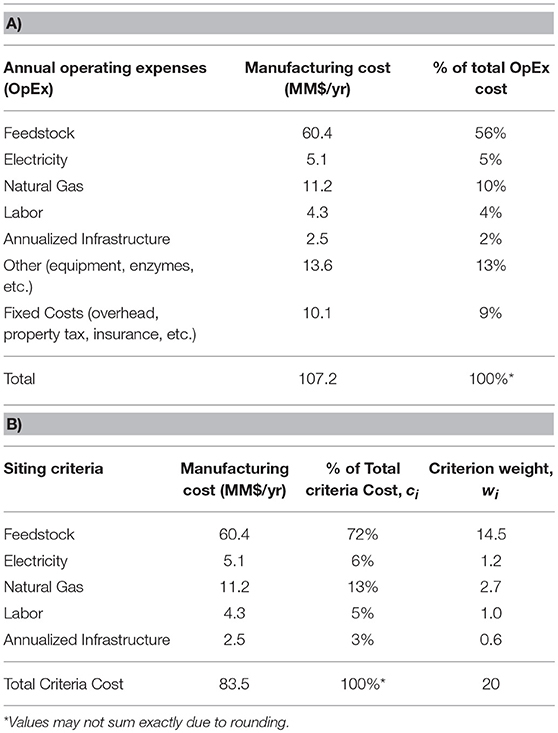
Table 7. (A) Biorefinery operational expenses and (B) Conversion to decision matrix weights.

Weights for the biorefinery decision matrix are developed using Equation (1). Regional average energy rates are input into the biorefinery TEA. The feedstock cost for the TEA (Equation 13) is the average of all potential biorefinery weighted average delivered feedstock costs (Equation 14).

$\begin{array}{rc}T{C}_{bjk}=P{C}_j+T{C}_{jk}& (13)\end{array}$

$\begin{array}{rc}W{A}_k=\frac{\left({\displaystyle {\sum }_{i=1}^y}T{C}_{bjk}{B}_j\right)}{B_k}& (14)\end{array}$

where TC_bjk is the total delivered feedstock cost from depot j to biorefinery k, PC_j is the processing cost, or minimum selling price, of micronized wood at depot j, TC_jk is the transportation cost to deliver micronized wood to biorefinery k, B_j is the volume of feedstock at depot j, B_k is the total volume of feedstock to meet biorefinery demand, and y is the total number depots in the depot-and biorefinery supply chain. PC_j is determined from the depot TEA by inputting depot-specific weighted average delivered feedstock cost and energy rates, which results in a final unit cost to produce one BDMT of milled wood plus profit. To determine the “facility infrastructure” criterion weight, the design biorefinery's total capital cost for construction, as identified in the TEA, is converted to an annualized cost assuming a plant life of 20 years and a discount rate of 8% (Martinkus et al., 2017b).

One decision matrix is developed to assess all three depot-and-biorefinery supply chains so the least-cost supply chain may be identified. Bin values for energy and labor rates are the same as for the depot decision matrix, as the region definition is the same. Feedstock is now measured by the weighted average total delivered feedstock cost of the two satellite depots and one large depot to the biorefinery gate (WA_k) plus the cost to transport biofuel to the petroleum terminal (TC_kl). Processing costs at the biorefinery are not included as they are reflected in the siting criteria. The range of facility values for feedstock and infrastructure assessment are used for their respective bin value determinations. Scoring and ranking of the proposed biorefinery supply chains is performed using the biorefinery decision matrix (Table 8A).

TABLE 8

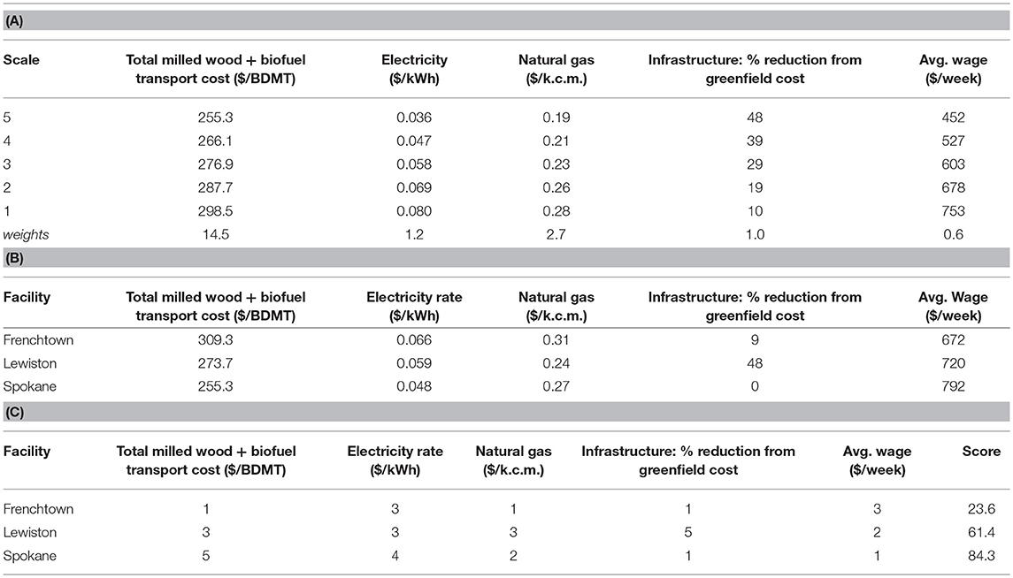
Table 8. (A) Biorefinery decision matrix, (B) Location-specific values, and (C) Scaled values with final facility scores.

Results and Sensitivity Analysis

Table 8 displays the biorefinery decision matrix and facility assessments. Spokane was found to be the least-cost location for processing feedstock into aviation biofuel, although it is a greenfield. Infrastructure was not found to be a significant annual expense due to pretreatment occurring in the depots and not at the biorefinery, as seen in the infrastructure criteria weight of 1.0. As evidenced in Figure 3, Spokane is centrally located among large amounts of biomass and near depots with lesser energy rates, while Frenchtown incurs the greatest expenses due to higher energy rates and its remote location, which increases transportation costs. It must be noted that the feedstock costs in Table 8B are higher than an integrated biorefinery would pay for raw feedstock due to the milled wood being pretreated and the bulk density increased at the depot. Thus, the cost for pretreatment is not represented in the capital and operational expenditures of the biorefinery, but in the cost for feedstock.

A sensitivity analysis was performed to assess the variables and assumptions that influence the decision matrix results, including biomass availability, bin designations, and weights. Additionally, the decision matrix results are compared against an optimization routine to assess the accuracy of the matrix at selecting depots for each supply chain, and the least-cost supply chain for supplying the Spokane market with aviation biofuel.

Sensitivity Analysis

Biomass Availability

Biomass availability is a function of biomass supply and the trucking assumptions represented in the TTCM. Biomass supply is considered to have a medium uncertainty due to the many variables that comprise it, including the seasonality of harvest operations and the amount of residue available and accessible at varying slopes and distances from the forest landing (Miller and Boston, 2017). Similar to Martinkus et al. (2017a), a high feedstock cost scenario was run to determine the increase in feedstock cost each biorefinery may incur to meet annual demand during years of low biomass availability. A low-cost scenario was run assuming the use of a blower for loading ground chips into the chip van at the forest landing, which was found to increase payload by 25% over traditional gravity-fed loading methods (Zamora-Cristales et al., 2014). The resulting delivered feedstock costs for each top-ranked depot were input into the depot TEA along with their respective electricity and natural gas rates to determine the revised fixed cost at each depot. This fixed cost was summed with the transport cost for hauling the micronized wood to each respective biorefinery to determine the total delivered feedstock cost (Equation 13, Figure 4).

FIGURE 4

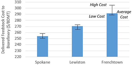
Figure 4. Biomass sensitivity analysis with low-cost, average, and high-cost results.

The fixed cost at the forest landing is based on an assumed off-road diesel cost, equipment types and efficiencies, and a landowner payment assuming a weak market for forest residue. The variable cost for residue transport to depots is based on a 30-year average diesel cost of $0.93/liter and a set chip van size. Han and Murphy (2011) found that a 10 percent increase in fuel cost resulted in a 3 percent increase in total transportation costs. The fixed and variable costs for the forest-to-depot linkage are used with low uncertainty, as time-motion studies were performed to develop the costs (Zamora-Cristales et al., 2013, 2015). The fixed and variable costs for the linkages between the depots, biorefineries, and petroleum terminal are used with medium uncertainty, as one reference was used (Parker et al., 2008) to develop the tanker truck total cost equation and only a diesel cost of $0.66/liter was provided as insight into their cost derivations. The rail costs from Parker et al. (2008) were compared against other sources (Gonzales et al., 2013; Lewis et al., 2015; USDA Agriculture Marketing Service, 2015) and determined to be mid-range among all costs and therefore acceptable for use.

Bin Designations

The importance of region definition on bin designations was assessed through evaluating energy averages in the region defined by all counties in Oregon, Washington, Idaho, and Montana (here called the Pacific Northwest, or PNW). The electricity average increases marginally, from $0.061 to $0.064/kWh for the PNW, with the increase in region boundary size, while the natural gas average decreases slightly from $0.27 to $0.25/k.c.m. for the PNW. While the means did not change significantly, the minimum and maximum values for each is noticeably different. The PNW electricity range was $0.028 to $0.131/kWh while the study region range was $0.036/kWh to $0.091/kWh. Similarly, the PNW natural gas range was $0.16 to $0.33/k.c.m while the study region range was $0.19 to $0.31/k.c.m. The difference in range affects bin designations in the decision matrices, and thus affects the spread of scaled values. If the PNW range was used in this analysis, the facility scaled values would lose their granularity due to the larger range of values, and thus more facilities would be assigned the same scale value. Electricity, natural gas, and labor rates all come from reputable government agencies and are considered to have low uncertainty.

Weighting Analysis

A weight sensitivity analysis was performed by varying the cost of feedstock, electricity, and natural gas rates (Table 9). In the depot decision matrix, the only major change in weights occurs when electricity is set at the lowest rate in the study region. Electricity is the highest annual cost in the depot TEA; by lowering the rate substantially, feedstock then becomes the highest annual cost. In the biorefinery TEA, feedstock cost is significantly higher than all other costs, therefore an increase in electricity or natural gas rates is not significant in overall weighting.

TABLE 9

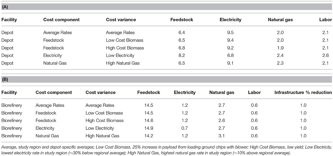
Table 9. Weighting sensitivity analysis for (A) depot and (B) biorefinery decision matrices.

Labor was not assessed because national average salaries were used for the various positions identified in the TEAs (such as plant engineer, shift supervisor, yard employees, etc.) as opposed to using county-level labor rates to calculate annual wages. Additionally, changes in the percent reduction in infrastructure was not assessed. Both of these criteria are low cost components in the overall annual cost to operate the depot or biorefinery, therefore changes in their values would not significantly affect the other weights, as evidenced by evaluating a high natural gas rate.

Validation of Decision Matrix Results

An optimization routine using binary integer programming was created to identify the top two satellite depots for each biorefinery as a comparison against the depots selected by the decision matrix. The Supplemental Information describes the optimization routine. The optimization model minimizes total cost for each scenario including the total annual cost to procure, purchase, process, and transport the biomass/biofuel to the end user. The difference between this minimum cost and the total cost associated with the depots selected by the decision matrix represents the opportunity cost, or forgone value, of the approach. The results are displayed in Table 10. The optimization model and depot decision matrix were in agreement for the depots selected for Lewiston, ID, and were only marginally different in total cost for the depots selected for Spokane, WA. The depots selected by the decision matrix for Frenchtown, MT would increase the total cost to operate the supply chain over the optimization model results by close to $1 million dollars, however this equates to only a 1% increase in total annual cost over the optimized supply chain.

TABLE 10

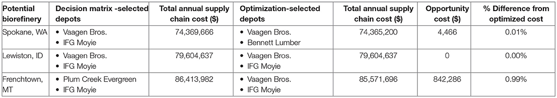
Table 10. Comparison of decision matrix and optimization model depot selections and total annual supply chain cost.

Discussion

The results of the optimization comparison (Table 10) show the strength of the decision matrix in its ability to take the complex issue of multiple cost variables at a given site and simplify it through applying weights to the costs based on their importance in the facility's operating budget. The Spokane supply chain had the least annual cost of the potential biorefineries, and thus would most likely be the best location for a biorefinery. The optimization run for Spokane selected the second and third depots from the decision matrix ranking list, for Frenchtown it selected the second and fourth depots from the list, and for Lewiston, the top two depots were identified as optimal (Tables 6, 10). Vaagen Brothers and IFG Moyie were consistently selected as top depots for each supply chain due to their ease of procuring feedstock and low electricity rate, respectively. These results, combined with the percent difference from optimized cost (Table 10), validate the use of the decision matrix as a strategic-level facility siting tool for identifying the top depots that provide biomass to a facility at the least cost. Stakeholders interested in using the decision matrix for biorefinery supply chain development would engage representatives from the top few-selected depots in discussions around contracts and pricing, then from those conversations select the final depots for use in a depot-and-biorefinery supply chain.

Both the depot and biorefinery geospatial cost components comprise ~80% of their respective total facility operational costs (Tables 2, 7). Thus, their use as siting criteria is relevant for assessing each potential facility's location-specific cost components and the effect it has on the total annual amount spent on operational costs. The assessment of high-cost biomass gives an indication of the additional amount biorefineries may pay during years of low feedstock availability, and the low-cost assessment shows how technological advances can translate into reduced feedstock costs at the depot mill gate. Figure 4 indicates that Frenchtown is the most vulnerable to years of high biomass cost since it exhibits the largest range in feedstock pricing. The Spokane biorefinery would operate at lower costs than Lewiston or Frenchtown, even during years of low biomass availability, as evidenced by the compactness of its biomass procurement and transporting in Figure 4.

Region definition plays an important role in bin designations and therefore in facility scores. When regions are defined to be much larger than the study area, the range of each bin may increase with an increase in the minimum and maximum values for each criterion. This may result in more facilities being assigned the same scale values, and thus will reduce the range of facility scores.

Just as rates and assets vary geospatially, the annual amount spent on each cost component varies based on the design of the depot and biorefinery. For example, wood-based integrated biorefineries require significant amounts of electricity and natural gas for preprocessing woody biomass into pulp (Zhu and Zhuang, 2012), whereas biorefineries in a depot model require less energy due to preprocessing occurring at depots. The feedstock cost at the biorefinery gate in this analysis was larger than would be expected at an integrated biorefinery; however, the feedstock cost reflects the cost of pretreatment occurring at the depots. While the feedstock cost is larger, the capital and operational costs of the biorefinery are less than an integrated biorefinery due to the disaggregation of pretreatment from the facility. This was evidenced by the selection of Spokane as the least-cost location to construct a biorefinery, even though it is a greenfield. The annualized infrastructure (capital cost) to construct the biorefinery was around 2% of the total operational costs (Table 7), whereas in an integrated biorefinery, infrastructure may play a larger role as pretreatment can be a significant capital cost depending on the conversion technology. Additionally, feedstock costs are a function of the size and number of depots used in the supply chain model. This analysis was based on the a priori assumption of two small satellite depots and one large co-located depot at the biorefinery. Additional modeling through either optimization runs or varying the assumption of depot size and number, and creating decision matrices that reflect these assumptions, will allow for identification of the depot-and-biorefinery configuration that provides the least overall supply chain costs. As depots become larger, economies of scale allow for more efficient processing of biomass, which is seen in a lower minimum selling price of preprocessed biomass to the biorefinery. Larger depots may equate to fewer depots in a supply chain, which can lessen transportation costs to the biorefinery as well. Cost sharing that may occur between depots and primary processors through co-location was not modeled here. Significant depot operational cost savings may be gained through sharing of staff, energy, residuals, etc.; however, further research is necessary to quantify these potential cost savings.

Similar to Richardson et al. (2011), we found that fixed costs account for a significant portion of the delivered feedstock cost from the forest to the depot. Technological advances may reduce this cost. However, as the biomass market becomes commercialized, landowner payments may increase (U.S. Department of Energy, 2011) and processing costs may decrease due to economies of scale. Rail was found to be utilized only for the furthest depot from the biorefinery in each supply chain analysis. This is consistent with personal communication with members of the freight industry that say rail is not feasible until ~320 km.

The TEAs are constructed using ratio factors from methodology presented by Peters et al. (2003) to estimate total capital investment. Operational and capital expenses are estimated from equipment quotes and literature references. An economic analysis with a real discount rate of 10 and 2% inflation was used to determine minimum selling price of both the micronized wood and aviation biofuel (Petter and Tyner, 2014).

The decision matrices presented here require depot and biorefinery sizes to be selected a priori. The most likely scenario for use would be stakeholders that want to identify potential depots for pre-selected potential biorefineries with a given annual feedstock demand. If using an optimization routine is not feasible for selecting the optimal size and location of facilities, then multiple iterations of the decision matrices may be run to assess the change in cost of the depot-and-biorefinery supply chain with different sized facilities. This requires the use of multiple TEAs, as each TEA is built for a specific facility size. The biorefinery decision matrix can also be used independently for siting an integrated biorefinery, as performed by Martinkus et al. (2017b).

Overall, the proposed decision matrix design performs well as a facility site selection tool. The advantage of the tool is its simplicity in identifying, combining, and weighting cost components that most affect the overall cost to construct and operate a facility. While the decision matrix was shown to perform well against more a complex optimization model, one disadvantage is that optimization modeling is still necessary to assign biomass source points to the final selected depots to estimate the delivered feedstock cost. Additionally, a TEA for each facility type (i.e., depot, biorefinery) is needed to perform siting criteria identification and analysis. Many TEAs exist online for biorefinery types, yet not all technologies are represented and location specific details are not always stated explicitly. Finally, the repurpose potential of existing facilities may be difficult to estimate. Information used to determine the presence or absence of equipment and assets at each facility may be located in national/state sources or datasets and from aerial imagery (Martinkus and Wolcott, 2017).

Conclusions

We propose a quantitative facility siting tool to identify the least-cost regional biorefinery supply chain from an array of potential depot and biorefinery locations. Co-location and repurpose strategies are assumed for existing primary processors and pulp mills, respectively, as a means to reduce capital and operational costs. Decision matrices provide a quantitative, transparent MCDA tool for assessing and prioritizing the various operational cost components that are present at each site. A total transportation cost model is utilized to quantify the feedstock procurement and processing costs at each linkage of the supply chain. An optimization routine validated the results of the decision matrices in the selection of depots for each biorefinery, and for selecting the least-cost depot-and-biorefinery supply chain.

By performing facility siting through assigning weights for feedstock, energy, and labor costs based on their importance in the operational costs of the facility, biorefinery supply chain development can be better directed to select facilities that provide the greatest cost reductions. Any cost reductions gained during the early phase of commercialization may translate into a more cost-competitive biofuel for cellulosic and advanced biorefineries.

Author Contributions

NM wrote the paper, created the decision support tools, developed all datasets needed to populate the decision matrices, and ran the siting analyses and sensitivity analyses to determine the best location for a biorefinery. GL created the LURA model and ran the model to determine 20-year average forest residue volumes at all FIA points used as biomass source points. GL also created and ran the optimization model to validate the results from the decision matrices. KB developed the TEAs that were used in the siting analyses for the determination of operational and capital costs at each facility. MW provided project oversight and review of the paper.

Conflict of Interest Statement

The authors declare that the research was conducted in the absence of any commercial or financial relationships that could be construed as a potential conflict of interest.

Acknowledgments

The authors gratefully acknowledge funding from the Northwest Advanced Renewables Alliance (NARA), supported by the Agriculture and Food Research Initiative Competitive Grant no. 2011-68005-30416 from the USDA National Institute of Food and Agriculture. This research was also funded by the U.S. Federal Aviation Administration Office of Environment and Energy through ASCENT, the FAA Center of Excellence for Alternative Jet Fuels and the Environment, project COE-2014-01 through FAA Award Number 13-C-AJFE-WaSU under the supervision of James Hileman and Nathan Brown. Any opinions, findings, conclusions or recommendations expressed in this material are those of the authors and do not necessarily reflect the views of the FAA.

Supplementary Material

The Supplementary Material for this article can be found online at: https://www.frontiersin.org/articles/10.3389/fenrg.2018.00124/full#supplementary-material

Abbreviations

BDMT, Bone Dry Metric Tons; CapEx, Capital Expenditure; DST, Decision Support Tool; FIA, Forest Inventory and Analysis; GIS, Geographic Information System; LURA, Land Use Resource Allocation; MCDA, Multi-Criteria Decision Analysis; OpEx, Operational Expenditure; TEA, Techno-Economic Analysis; TTCM, Total Transportation Cost Model

References

Argo, A., Tan, E., Inman, D., Langholtz, M., Eaton, L., Jacobson, J., et al. (2013). Investigation of biochemical biorefinery sizing and environmental sustainability impacts for conventional bale system and advanced uniform biomass logistics designs. Biofuel Bioprod. Bior. 7, 282–302. doi: 10.1002/bbb.1391

CrossRef Full Text | Google Scholar

Bals, B. D., and Dale, B. E. (2012). Developing a model for assessing biomass processing technologies within a local biomass processing depot. Bioresour. Technol. 106, 161. doi: 10.1016/j.biortech.2011.12.024

PubMed Abstract | CrossRef Full Text | Google Scholar

Brandt, K. L., Gao, J., Wang, J., Wooley, R. J., and Wolcott, M. (2018). Techno-economic analysis of forest residue conversion to sugar using three-stage milling as pretreatment. Front. Energy Res. 6:77. doi: 10.3389/fenrg.2018.00077

CrossRef Full Text | Google Scholar

Carolan, J. E., Joshi, S. V., Dale, B. E., Carolan, J. E., Joshi, S. V., and Dale, B. E. (2007). Technical and financial feasibility analysis of distributed bioprocessing using regional biomass pre-processing centers. J. Agric. Food Indus. Org. 5, 1–29. doi: 10.2202/1542-0485.1203

CrossRef Full Text | Google Scholar

Chung, W., and Anderson, N. (2012). “Spatial modeling of potential woody biomass flow,” in 35th Annual Meeting of the Council on Forest Engineering: Engineering New Solutions for Energy Supply and Demand, ed J. Roise (New Bern, NC).

Google Scholar

Coyle, W. T. (2010). Next-Generation Biofuels Near-Term Challenges and Implications for Agriculture. Washington, DC: U.S. Department of Agriculture Economic Research Service.

Dijkstra, E. W. (1959). A note on two problems in connexion with graphs. Numerische Mathematik 1, 269–271.

Google Scholar

Eranki, P., Bals, B., and Dale, B. (2011). Advanced Regional Biomass Processing Depots: a key to the logistical challenges of the cellulosic biofuel industry. Biofuel Bioprod. Bior. 5:10. doi: 10.1002/bbb.318

CrossRef Full Text | Google Scholar

Esri (2015). Algorithms Used by the ArcGIS Network Analyst Extension [Online]. Redlands, CA. Available: http://resources.arcgis.com/en/help/main/10.2/index.html#//004700000053000000 (Accessed 10/16/2015).

Federal Aviation Administration (2016). Terminal Area Forecast. Washington, DC: Federal Aviation Administration.

Fortenbery, T., Deller, S. C., and Amiel, L. (2013). The Location Decisions of Biodiesel Refineries. Land Econ. 89, 118–136.

Google Scholar

Gao, J., and Neogi, A. (2015). Clean Sugar and Lignin Pretreatment Technology Task 3: Tandem Wood Milling. NARA Final Reports, Northwest Advanced Renewables Alliance (NARA), Pullman, WA.

Gonzales, D., Searcy, E. M., and Ekşioğlu, S. D. (2013). Cost analysis for high-volume and long-haul transportation of densified biomass feedstock. Transport. Res. Part A. 49, 48–61. doi: 10.1016/j.tra.2013.01.005

CrossRef Full Text | Google Scholar

Graham, R. L., English, B. C., and Noon, C. E. (2000). A Geographic Information System-based modeling system for evaluating the cost of delivered energy crop feedstock. Biomass Bioenerg. 18, 309–329. doi: 10.1016/S0961-9534(99)00098-7

CrossRef Full Text | Google Scholar

Han, S.-K., and Murphy, G. (2011). Trucking productivity and costing model for transportation of recovered wood waste in Oregon. For. Prod. J. 61, 552–560. doi: 10.13073/0015-7473-61.7.552

CrossRef Full Text | Google Scholar

Hansen, J. K., Jacobson, J. J., and Roni, M. S. (2015). “Quantifying supply risk at a cellulosic biorefinery,” in 33rd International Conference of the System Dynamics Society (Cambridge, MA).

Google Scholar

Hawkins, A., and Ley, J. (2016). Production of Lignocellulosic Isobutanol by Fermentation and Conversion to Biojet. NARA Final Reports, Northwest Advanced Renewables Alliance (NARA), Pullman, WA.

Kenkel, P. L., and Holcomb, R. B. (2006). Challenges to producer ownership of ethanol and biodiesel production facilities. J. Agric. Appl. Econ. 38, 369–375. doi: 10.1017/S1074070800022410

CrossRef Full Text | Google Scholar

Kim, S., and Dale, B. E. (2015). Comparing alternative cellulosic biomass biorefining systems: Centralized versus distributed processing systems. Biomass Bioenerg. 74, 135–147. doi: 10.1016/j.biombioe.2015.01.018

CrossRef Full Text | Google Scholar

Kocoloski, M., Griffin, W., and Matthews, H. (2011). Impacts of facility size and location decisions on ethanol production cost. Energy Policy 39, 47–56. doi: 10.1016/j.enpol.2010.09.003

CrossRef Full Text | Google Scholar

Lamers, P., Roni, M. S., Tumuluru, J. S., Jacobson, J. J., Cafferty, K. G., Hansen, J. K., et al. (2015a). Techno-economic analysis of decentralized biomass processing depots. Bioresour. Technol. 194, 205–213. doi: 10.1016/j.biortech.2015.07.009

PubMed Abstract | CrossRef Full Text | Google Scholar

Lamers, P., Tan, E. C. D., Searcy, E. M., Scarlata, C. J., Cafferty, K. G., and Jacobson, J. J. (2015b). Strategic supply system design – a holistic evaluation of operational and production cost for a biorefinery supply chain. Biofuel Bioprod. Bior. 9, 648–660. doi: 10.1002/bbb.1575

CrossRef Full Text | Google Scholar

Latta, G. S., Baker, J. S., and Ohrel, S. (2018). A Land Use and Resource Allocation (LURA) modeling system for projecting localized forest CO₂ effects of alternative macroeconomic futures. For. Policy Econ. 87, 35–48. doi: 10.1016/j.forpol.2017.10.003

CrossRef Full Text | Google Scholar

Lewis, K. C., Baker, G., Lin, T. T., Smith, S., Gillham, O., Fine, A., et al. (2014). Biofuel Transportation Analysis Tool: Description, Methodology, and Demonstration Scenarios. Washington, DC: Office of Environment and Energy & Office of Naval Research.

Google Scholar

Lewis, K. C., Baker, G. M., Pearlson, M. N., Gillham, O., Smith, S., Costa, S., et al. (2015). Alternative Fuel Transportation Optimizatin Tool: Description, Methodology, and Demonstration Scenarios. Washington, DC: John A Volpe National Transportation Systems Center.

Ma, J., Scott, N. R., Degloria, S. D., and Lembo, A. J. (2005). Siting analysis of farm-based centralized anaerobic digester systems for distributed generation using GIS. Biomass Bioenerg. 28, 591–600. doi: 10.1016/j.biombioe.2004.12.003

CrossRef Full Text | Google Scholar

Macfarlane, R., Mazza, P., and Allan, J. (2011). Sustainable Aviation Fuels Northwest: Powering the Next Generation of Flight. Seattle, WA: Sustainable Aviaton Fuels Northwest.

Marrs, G., Spink, T., and Gao, A. (2016). Process Design and Economics for Biochemical Conversion of Softwood Lignocellulosic Biomass to Isoparaffinic Kerosene and Lignin Co-products. NARA Final Reports, Northwest Advanced Renewables Alliance (NARA), Pullman, WA.

Martinkus, N., Latta, G., Morgan, T., and Wolcott, M. (2017a). A comparison of methodologies for estimating delivered forest residuals volume and cost to a wood-based biorefinery. Biomass Bioenerg. 106, 83–94. doi: 10.1016/j.biombioe.2017.08.023

CrossRef Full Text | Google Scholar

Martinkus, N., Rijkhoff, S. A. M., Hoard, S. A., Shi, W., Smith, P., Gaffney, M., et al. (2017b). Biorefinery site selection using a stepwise biogeophysical and social analysis approach. Biomass Bioenerg. 97, 139–148. doi: 10.1016/j.biombioe.2016.12.022

CrossRef Full Text | Google Scholar

Martinkus, N., and Wolcott, M. (2017). A framework for quantitatively assessing the repurpose potential of existing industrial facilities as a biorefinery. Biofuel Bioprod. Bior. 11, 295–306. doi: 10.1002/bbb.1742

CrossRef Full Text | Google Scholar

Miller, C., and Boston, K. (2017). The quantification of logging residues in oregon with impacts on sustainability and availability of raw material for future biomass energy. Eur. J. For. Eng. 3, 16–22.

Google Scholar

Ng, R. T. L., and Maravelias, C. T. (2016). Design of cellulosic ethanol supply chains with regional depots. Ind. Eng. Chem. Res. 55, 3420–3432. doi: 10.1021/acs.iecr.5b03677

CrossRef Full Text | Google Scholar

Noon, C., Zhan, F. B., and Graham, R. L. (2002). GIS based analysis of marginal price variation with an application in the identification of candidate ethanol conversion plant locations. Netw. Spat. Econ. 2, 79–93. doi: 10.1023/A:1014519430859

CrossRef Full Text | Google Scholar

Panichelli, L., and Gnansounou, E. (2008). GIS-based approach for defining bioenergy facilities location: A case study in Northern Spain based on marginal delivery costs and resources competition between facilities. Biomass Bioenerg. 32, 289–300. doi: 10.1016/j.biombioe.2007.10.008

CrossRef Full Text | Google Scholar

Parker, N., Tittman, P., Hart, Q., Lay, M., Cunningham, J., and Jenkins, B. (2008). Strategic Assessment of Bioenergy Development in the West: Spatial Analysis and Supply Curve Development. The University of California, Davis, CA.

Perimenis, A., Walimwipi, H., Zinoviev, S., Müller-Langer, F., and Miertus, S. (2011). Development of a decision support tool for the assessment of biofuels. Energ. Policy 39, 1782–1793. doi: 10.1016/j.enpol.2011.01.011

CrossRef Full Text | Google Scholar

Peters, M. S., Timmerhaus, K. D., and West, R. E. (2003). Plant Design and Economics for Chemical Engineers. New York, NY: McGraw-Hill.

Google Scholar

Petter, R., and Tyner, W. E. (2014). Technoeconomic and policy analysis for corn stover biofuels. ISRN Econ. 2014:515898. doi: 10.1155/2014/515898

CrossRef Full Text

Richardson, J. J., Spies, K. A., Rigdon, S., York, S., Lieu, V., Nackley, L., et al. (2011). Uncertainty in biomass supply estimates: lessons from a Yakama Nation case study. Biomass Bioenerg. 35, 3698–3707. doi: 10.1016/j.biombioe.2011.05.030

CrossRef Full Text | Google Scholar

Saaty, T. L. (2008). Decision making with the analytic hierarchy process. Int. J. Serv. Sci. 1, 83–98. doi: 10.1504/IJSSci.2008.01759

CrossRef Full Text | Google Scholar

Stephen, J. D., Sokhansanj, S., Bi, X., Sowlati, T., Kloeck, T., Townley-Smith, L., et al. (2010). Analysis of biomass feedstock availability and variability for the Peace River region of Alberta, Canada. Biosyst. Eng. 105, 103–111. doi: 10.1016/j.biosystemseng.2009.09.019

CrossRef Full Text | Google Scholar

Stewart, L., and Lambert, D. M. (2011). Spatial heterogeneity of factors determining ethanol production site selection in the US, 2000-2007. Biomass Bioenerg. 35, 1273–1285. doi: 10.1016/j.biombioe.2010.12.020

CrossRef Full Text | Google Scholar

Sultana, A., and Kumar, A. (2012). Optimal siting and size of bioenergy facilities using geographic information system. Appl. Energy 94, 192–201. doi: 10.1016/j.apenergy.2012.01.052

CrossRef Full Text | Google Scholar

U.S. Bureau of Labor Statistics (2015). Quarterly Censuys of Employment and Wages. 06-02-2015 ed. U.S. Department of Labor, Washington, DC.

U.S. Department of Energy (2011). U.S. Billion-Ton Update: Biomass Supply for a Bioenergy and Bioproducts Industry, eds R. D. Perlack and B. J. Stokes (Leads), Oak Ridge National Laboratory, Oak Ridge, TN.

U.S. Energy Information Administration (2014a). Electric Power Sales, Revenue, and Energy Efficiency Form EIA-861 Detailed Data Files. U.S. Energy Information Administration, Washington, DC.

U.S. Energy Information Administration (2014b). Natural Gas Annual Respondent Query System. U.S. Energy Information Administration, Washington, DC.

United States Forest Service (2016). Forest Inventory and Analysis National Program [Online]. Available online at: http://www.fia.fs.fed.us/ (Accessed May 12, 2016).

USDA Agriculture Marketing Service (2015). Biofuels and Co-products Datasets. October 2015 ed. U.S. Department of Agriculture, Washington, DC.

Van Dael, M., Van Passel, S., Pelkmans, L., Guisson, R., Swinnen, G., and Schreurs, E. (2012). Determining potential locations for biomass valorization using a macro screening approach. Biomass Bioenerg. 45, 175–186. doi: 10.1016/j.biombioe.2012.06.001

CrossRef Full Text | Google Scholar

Wang, J., Gao, J., Brandt, K. L., Jiang, J., Liu, Y., and Wolcott, M. P. (2018). Improvement of enzymatic digestibility of wood by a sequence of optimized milling procedures with final vibratory tube mills for the amorphization of cellulose. Holzforschung 72, 435–441. doi: 10.1515/hf-2017-0161

CrossRef Full Text | Google Scholar

Wang, J.-J., Jing, Y.-Y., Zhang, C.-F., and Zhao, J.-H. (2009). Review on multi-criteria decision analysis aid in sustainable energy decision-making. Renew. Sust. Energ. Rev. 13, 2263–2278. doi: 10.1016/j.rser.2009.06.021

CrossRef Full Text | Google Scholar

Wilson, B. S. (2009). Modeling Cellulosic Ethanol Plant Location Using GIS. Masters, University of Tennessee, Knoxville, TN.

You, F., Tao, L., Graziano, D. J., and Snyder, S. W. (2012). Optimal design of sustainable cellulosic biofuel supply chains: multiobjective optimization coupled with life cycle assessment and input–output analysis. AIChE J. 58, 1157–1180. doi: 10.1002/aic.12637

CrossRef Full Text | Google Scholar

Zamora-Cristales, R., Sessions, J., Boston, K., and Murphy, G. (2015). Economic optimization of forest biomass processing and transport in the Pacific Northwest USA. For. Sci. 61, 220–234. doi: 10.5849/forsci.13-158

CrossRef Full Text | Google Scholar

Zamora-Cristales, R., Sessions, J., Murphy, G., and Boston, K. (2013). Economic impact of truck- machine interference in forest biomass recovery operations on steep Terrain. For. Prod. J. 63, 162–173. doi: 10.13073/FPJ-D-13-00031

CrossRef Full Text | Google Scholar

Zamora-Cristales, R., Sessions, J., Smith, D., and Marrs, G. (2014). Effect of high speed blowing on the bulk density of ground residues. For. Prod. J. 64, 290. doi: 10.13073/FPJ-D-14-00005

CrossRef Full Text | Google Scholar

Zhang, F., Johnson, D. M., and Sutherland, J. W. (2011). A GIS- based method for identifying the optimal location for a facility to convert forest biomass to biofuel. Biomass Bioenerg. 35, 3951–3961. doi: 10.1016/j.biombioe.2011.06.006

CrossRef Full Text | Google Scholar

Zhu, J. Y., and Zhuang, X. S. (2012). Conceptual net energy output for biofuel production from lignocellulosic biomass through biorefining. Prog. Energy Combust. 38, 583–598. doi: 10.1016/j.pecs.2012.03.007

CrossRef Full Text | Google Scholar