Methanol Production via CO2 Hydrogenation: Sensitivity Analysis and Simulation—Based Optimization

Introduction

Most of energy in the world is currently from combustion of carbonaceous fuels, which are coal, oil, and natural gas. CO₂ emission from this combustion is considered as the second contribution to the greenhouse effect (9–26%), after the water vapor and clouds (36–72%). The recent attempts predict that CO₂ will show stronger greenhouse effect when its amount in the atmosphere is double (Jaworowski et al., 1992). The net CO₂ emissions could increase at around 5.4% over the next few decades (Radhi, 2009). Due to this concern, many applications and researches on CO₂ conversion and utilization have been studied to control amount of CO₂ releasing to the atmosphere. CO₂ can either be used directly or as feedstock to produce useful chemicals and materials. For the direct use, CO₂ is utilized in many different applications such as food preservation, beverage carbonation, fire extinguisher, supercritical extraction, dry ice, etc (Song et al., 2002). For conversion of CO₂ to other products, urea synthesis is the largest production while the methanol synthesis is the second largest production in this area (Naims, 2016).

Methanol is commonly used as both solvent and reactant in chemical industry. Uses of methanol is found in many household products, including paints, varnishes, cleaning products (Dasgupta and Klein, 2014). Moreover, methanol can use as a motor fuel or gasoline blending component (Ingamells and Lindquist, 1975). The methanol—fueled vehicles use a blend of 85 percent methanol with 15 percent unleaded gasoline (M85) (Ingamells and Lindquist, 1975; EPA, 2002; Bukhtiyarova et al., 2017). From laboratory and road tests indicate that adding of 10% methanol can raise octane 2–3 numbers. In the research of Gabele (1990), the results showed that increase of methanol content does not affect the emission rate of exhaust gas.

In the conventional methanol production, methanol is produced from petroleum product (synthesis gas) via hydrogenation of CO and CO₂, and reversed water—gas shift reaction (María et al., 2013). The commercial methanol productions from synthesis gas use CuO/ZnO/Al₂O₃ as catalyst (Sayah et al., 2010; Jadhav et al., 2014). The commercial CuO/ZnO/Al₂O₃ coupled with a zeolite membrane reactor can provide higher CO₂ conversion, methanol yield, and selectivity compared with a traditional reactor (Gallucci et al., 2004). Copper based catalyst is mostly used for CO₂ hydrogenation to methanol due to its cheap and higher catalyst activity (Ali et al., 2015). Saito and Murata studied of Al₂O₃ supported Cu-based catalyst with Co-precipitation technique. The catalyst shows high activity and the stability was improved by adding colloidal silica (Saito and Murata, 2004).

Several developments of catalysts used in catalytic conversion to improve the performance of catalyst were studied. Mg and Mn was promoted on CuZnZr catalyst. Adding of MgO and MnO lead to increase in catalytic activity of the catalyst (Sloczyński et al., 2003). Doping of Mn to Cu/Zn/Zr catalyst can increase the methanol production rate. The zirconium indicates the advantageous influence on the catalyst activity (Lachowska and Skrzypek, 2004). The Pd/ZnO catalysts over multi-walled carbon nanotubes was found to have the turnover frequency reached 0.015 per second (Liang et al., 2009).

Recently, the production of methanol from direct CO₂ hydrogenation is of interest (Samimi et al., 2017; Marlin et al., 2018). The process has potential to mitigate the CO₂ emission to the atmosphere. The methanol production from direct CO₂ (using pure sources of CO₂ and H₂) has several advantages over the conventional process—it results in significantly less byproducts, and requires less energy in product purification (Marlin et al., 2018). However, the methanol production cost via direct CO₂ hydrogenation is 2–2.5 times higher than the cost of conventional process (Atsonics et al., 2015). The process of methanol production via CO₂ hydrogenation consumes more utilities than the conventional methanol production (Machado et al., 2014).

There are some studies on simulation—based optimization of methanol synthesis to increase the methanol production rate (Hoseiny et al., 2016; Leonzio, 2017). For methanol production from synthesis gas, the effects of changes in operating conditions on the production rate were studied to maximize the production rate. The studied operating parameters were feed flow rate, pressure and temperature of feed, and the cooling water temperature. The results showed that the methanol production rate can be increased by 7% with higher feed pressure and lower feed temperature (Hoseiny et al., 2016). For methanol synthesis via direct CO₂ hydrogenation, Grazia Leonzio developed mathematical model of the reactor used in methanol production. The impacts of reaction temperature, reaction pressure, H₂/CO₂ ratio, and the recycle factor on methanol production rate and reactor volume were studied (Leonzio, 2017).

However, optimization of methanol production via CO₂ hydrogenation, which considers all possible operating parameters, for the minimum production cost has not been studied. This paper studied an application of response surface methodology (RSM) in optimization of methanol production via CO₂ hydrogenation process. To be able to apply the RSM in optimization, the response surface has to be in the form of the second order model. The sensitivity analysis was used to determine the significant operating parameters. The RSM coupled with non-linear solver was employed to obtain the local optimal operating conditions and the minimum methanol production cost.

This paper is organized as follows: section Process simulation and economic evaluation gives details of process simulation and economic evaluation. Section Methodology provides methodology used in this work including details of sensitivity analysis and simulation—optimization framework. Section Results and discussion discusses results of process optimization. Section Conclusion provides conclusion.

Process Simulation and Economic Evaluation

In the study of methanol production process via CO₂ hydrogenation, the process simulation was combined with the economic analysis to evaluate the objective function (the methanol production cost) corresponding to the decision variables. In what follows, details of process simulation and economic evaluation are explained.

Process Simulation

The methanol production process via CO₂ hydrogenation was simulated using Aspen Hysys version 8.8 process simulator. Peng-Robinson was used as the thermodynamic property package. The physical properties were predicted using the thermodynamics based equation as shown in Equations (1) and (2). Where H^ID is the Ideal Gas Enthalpy and S^ID is the Ideal Gas Entropy.

$\begin{array}{ll}\frac{H-H^{ID}}{RT}=Z-1+\frac{1}{RT}{\displaystyle \underset{\infty }{\overset{V}{\int }}}\left[T{\left(\frac{\partial P}{\partial T}\right)|}_V-P\right]\text{d}V& (1)\end{array}$

$\begin{array}{ll}\frac{S-S_o^{ID}}{RT}=lnZ-ln\frac{P}{P^o}+{\displaystyle \underset{\infty }{\overset{V}{\int }}}\left[\frac{1}{R}{\left(\frac{\partial P}{\partial T}\right)|}_V-\frac{1}{V}\right]\text{d}V& (2)\end{array}$

In the process simulation, two reactors were employed due to low conversion of the CO₂ hydrogenation reaction. Figure 1 represents the process flow diagram of methanol production via CO₂ hydrogenation (Wiesberg et al., 2016). In this process, the feed of 1,000 kmoles per hour of carbon dioxide at 40°C and 20 bar was mixed with the 3,000 kmoles per hour of hydrogen (at the same conditions). The mixture was then compressed, heated and sent to the first equilibrium reactor. The first reactor partially converted CO₂ to methanol as liquid product, as shown in Equations (3)–(5) (Tidona et al., 2013). The unreacted CO₂ and H₂ then entered the second equilibrium reactor to produce more methanol product. The pressure of gas phase leaving the second reactor was reduced to recover methanol as liquid phase. All liquid methanol products were sent to the first distillation column, where the light components (CO, CO₂, and H₂) leaved at the top of the column. The mixture of methanol and water leaved the column at the bottom and entered the second distillation column, where the methanol product with purity of 99.5%mole was obtained at the top of the column.

$\begin{array}{ll}\text{C}{\text{O}}_2+{\text{H}}_2\leftrightarrow \text{C}\text{O}+{\text{H}}_2\text{O}\text{Δ}{\text{H}}_{300\text{K}}=41.2\text{k}\text{J}\text{p}\text{e}\text{r}\text{m}\text{o}\text{l}\text{C}{\text{O}}_2& (3)\end{array}$

$\begin{array}{ll}\text{CO}+2{\text{H}}_2\leftrightarrow \text{C}{\text{H}}_3\text{O}\text{H}\text{Δ}{\text{H}}_{300\text{K}}=-90.4\text{k}\text{J}\text{p}\text{e}\text{r}\text{m}\text{o}\text{l}\text{C}{\text{O}}_2& (4)\end{array}$

$\begin{array}{ll}\text{C}{\text{O}}_2+3{\text{H}}_2\leftrightarrow {\text{C}\text{H}}_3\text{O}\text{H}+\text{Δ}{\text{H}}_2\text{O}{\text{H}}_{300\text{K}}=-49.2\text{k}\text{J}\text{p}\text{e}\text{r}\text{m}\text{o}\text{l}\text{C}{\text{O}}_2& (5)\end{array}$

FIGURE 1

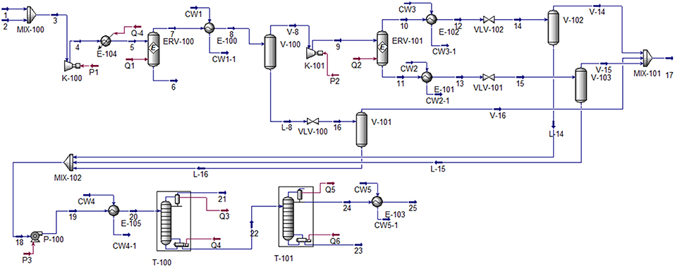
Figure 1. Simulation of methanol production via CO₂ hydrogenation process.

For equipment specifications, both reactors were simulated using equilibrium model. The sets of reaction used in each reactors are Equations (3)–(5). The efficiency of the pump was assumed at 75% (adiabatic). The efficiencies of all compressors were assumed at 75% (adiabatic). The specifications of column T−100 were condenser temperature at 40.1°C and reflux ratio at 0.5. The specifications of column T−101 were 99.5%mole methanol product purity, and reboiler temperature at 143.2°C.

The detailed process simulation of methanol production via CO₂ hydrogenation is provided in Appendix A.

Economic Evaluation

In an economic analysis, capital, and operating costs were included in calculation of methanol production cost. The capital cost involved all major equipment, except pump, and piping. The capital cost was calculated using equations and data from the capital equipment-costing program (Turton et al., 2003). The data was adjusted for inflation from year 2001–2017 by using values of the Chemical Engineering Plant Cost Index, CEPCI. The CEPCI value in 2001 is 297, and the CEPCI value in 2017 is 541.7 (Jenkins, 2018).

The equipment costs were estimated base on total module costs (C_TM), shown in Equation (6), where n represents the total number of pieces of equipment. C_BM is the bare module cost, which can be estimated from Equation (7)

$\begin{array}{ll}{C}_{TM}={\displaystyle \sum _{i=1}^n}{C}_{TM,i}=1.18{\displaystyle \sum _{i=1}^n}{C}_{BM,i}& (6)\end{array}$

$\begin{array}{ll}{\text{C}}_{\text{BM}}\text{ = }{\text{C}}_{\text{P}}{}^o({\text{B}}_1\text{ + }{\text{B}}_2{\text{F}}_{\text{M}}{\text{F}}_{\text{P}})& (7)\end{array}$

Where ${\text{C}}_{\text{P}}{}^o$ is the purchased cost for base conditions, which can be determined from Equation (8)

F_P is the pressure factor

F_M is the material factor

$\begin{array}{ll}{log}_{10}{\text{C}}_{\text{p}}^{\text{o}}={\text{K}}_1+{\text{K}}_2{log}_{10}(\text{A})+{\text{K}}_3{\left[{log}_{10}(\text{A})\right]}^2& (8)\end{array}$

In Equation (8), parameters A is the capacity or size parameter for the equipment, K₁, K₂, K₃ are the maximum and minimum values used in the correlation.

The description of major equipment, and K₁, K₂, and K₃ used in this studied are shown in Table 1.

TABLE 1

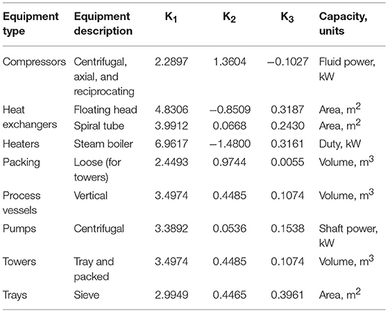
Table 1. Equipment description and parameter values.

For cost modeling of reactors, the dimension of reactors were fixed at height of 5.8674 m and diameter of 1.068 m. The values of K₁ is 3.4974, K₂ is 0.4485, K₃ is 0.1074, B₁ is 2.25, B₂ is 1.82, and F_M is 3.1. The pressure factors (Fp) for the reactors were determine using Equation (9), where P is in barg.

$\begin{array}{ll}{F}_{P,\text{vessel}}=\frac{\frac{(P+1)D}{2\left[850-0.6(P+1)\right]}+0.00315}{0.0063}\text{for }{\text{t}}_{\text{vessel}}>0.0063m& (9)\end{array}$

Assumption used in the economic analysis are listed below.

- The plant operates for 8,400 h per year.

- The plant is expected to have a 10—year plant life with on salvage value.

- The labor cost is $40,000 per operator per year.

- The working capital is 15% of fixed capital investment.

- Total capital investment including fixed capital investment and working capital.

- The maintenance and repairs are 5% of fixed capital investment.

- The operating supplies are 15% of maintenance and repairs.

- The laboratory charge is 15% of labor.

- The administrative expenses is 50% of labor cost.

- The maintenance and repairs, the laboratory charge and the administrative expenses increase annually 3%.

- The local taxes and insurance are 4% of fixed capital investment.

- The plant overhead cost is 60% of labor.

- The cost of carbon dioxide is $12.10 per ton (Wiesberg et al., 2016).

- The cost of hydrogen is $1,250 per ton (Wiesberg et al., 2016)

- The cost of process water at 25°C is $0.0259 per cubic meter.

- The cost of saturated steam at 6.9 bar is $55 per ton.

- The cost of electricity is $0.127 per kW h.

Methodology

The methodology in this work consists of two sections. The first section is “Sensitivity analysis” to determine the parameters that show significant impacts on the methanol production cost. The second section is “Simulation—Optimization” to optimize the significant operating parameters of methanol production process for the minimum methanol production cost. Details of Sensitivity analysis and Simulation—Optimization are described in the following sections.

Sensitivity Analysis

Sensitivity analysis is an efficient tool, which can be used to determine the significant parameters. In this section, the impacts of eight parameters on the methanol production cost were determined using sensitivity analysis. An increase in pressure and decrease in temperature leads to increase of the equilibrium conversion of CO₂ to methanol (Witoon et al., 2015). The eight studied parameters are (1 and 2) inlet pressure and temperature to the first reactor, ERV-100, for CO₂ and H₂ conversion conditions, (3) inlet temperature to the first separator for methanol product separation condition, (4) inlet pressure to the second reactor, ERV-101, for CO₂ and H₂ conversion conditions, (5 and 6) outlet temperature of both coolers, located after the second reactor, for methanol product separation condition from gas and liquid mixture, (7) outlet pressure at the valve VLV-102 for recovering methanol from gas phase mixture, (8) Inlet temperature to the first distillation column for separation between liquid methanol and water products, and gaseous unreacted reactant separation.

For all parameters, except inlet temperature to the first reactor, we performed the sensitivity analysis by varying value of interested parameter within the range ± 25% of its base value, and fixing other parameters at their base values. For inlet temperature to the first reactor parameter, we varied the value of temperature within the range ± 10% of its base value. Table 2 shows the base value used in sensitivity analysis of each parameter.

TABLE 2

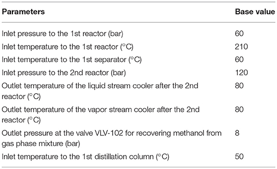
Table 2. Base case conditions used for sensitivity analysis.

Sensitivity Analysis: Results

The results from sensitivity analysis show that there are five parameters that show significant impacts on methanol production cost. Figure 2 shows inversely proportional relationship between operating parameters and methanol production cost (the methanol production cost decreases with an increase in the value of parameter). In the figure, the inlet pressure to the first reactor and the inlet temperature to the first distillation column show significant inversely proportional relationship with the methanol production cost.

FIGURE 2

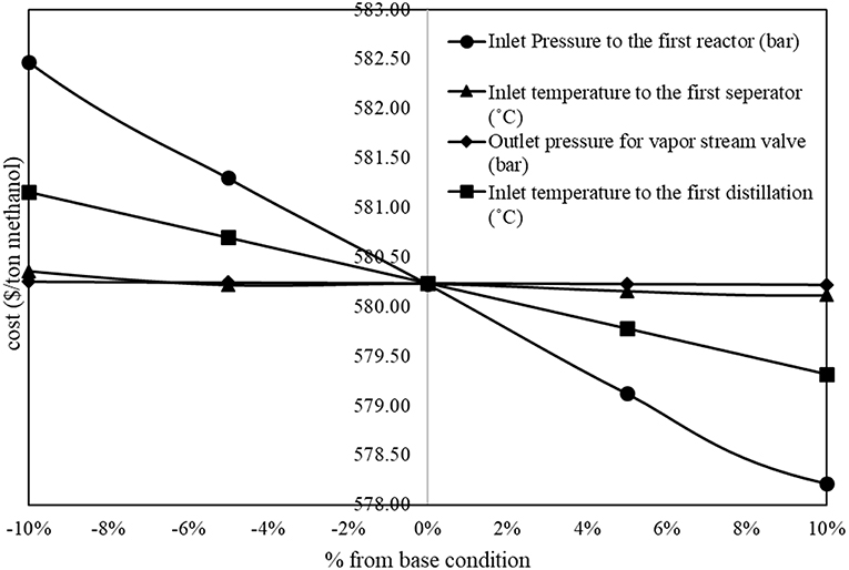
Figure 2. Inversely proportional relationship between parameters and methanol production cost.

On the other hand, Figure 3 shows proportional relationship between operating parameters and methanol production cost. In the figure, the inlet temperature to the first reactor, the inlet pressure to the second reactor, and the outlet temperature of the liquid stream cooler after the second reactor show significant proportional relationship to the methanol production cost.

FIGURE 3

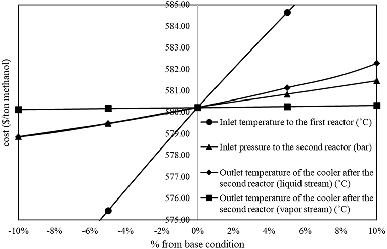
Figure 3. Proportional relationship between parameters and methanol production cost.

Five significant variables obtained from this sensitivity analysis will be used as decision variables to the optimization problem.

Simulation—Optimization

In this section, RSM (Nuchitprasittichai and Cremaschi, 2011) coupled with non-linear solver were employed to optimize the methanol production via CO₂ hydrogenation process. The objective is to minimize the methanol production cost per tons produced methanol ($/tons produced methanol). Response surface methodology is a statistical tool used to represent the relationship between independent variables and dependent variable(s). In this work, RSM was employed to represent the relationship between significant operating parameters and the methanol production cost per tons produced methanol. The significant operating parameters (decision variables) are the significant parameters obtained from sensitivity analysis (in section Sensitivity analysis) which are x₁: inlet pressure to the 1st reactor, x₂: inlet temperature to the 1st reactor, x₃: inlet pressure to the 2nd reactor, x₄: outlet temperature of the liquid stream cooler after the 2nd reactor, x₅: inlet temperature to the 1st distillation column.

Figure 4 represents simulation—optimization algorithm. In the algorithm, the range of each decision variables was first determined. In this work, the ranges of decision variables were obtained from literature (Shen et al., 2000; Witoon et al., 2015). Factorial design with two levels (2^k Factorial design, section 2^k Factorial design) and a center point were used as a data set of the decision variables. Then, process simulation, coupled with cost analysis, was run corresponding to operating conditions in the data set to obtained methanol production costs. The data of operating conditions and the corresponding methanol production costs were combined and fit the first order model by regression analysis (using Design Expert 11 software). If the data fit the first order model (R—squared > 0.7), it means that the region of operating conditions and methanol production costs is in linear region. The steepest descent (section Steepest descent) was performed to move operating conditions to the region of lower methanol production cost. On the other hand, if the data do not fit the first order model, it means that the data are in non-linear region. The Box—Behnken Design [BBD, section Box—Behnken design (BBD)] was performed to collect more data in non-linear region. All data were then combined to fit the second order (non-linear) model. The non-linear model was then used as the objective function in optimization problem. Microsoft Excel (non-linear programing, NLP) solver was used to solve the non-linear optimization problem (section Optimization formulation) for the minimum methanol production cost. The optimal solution obtained from this RSM is considered as a local optimal solution.

FIGURE 4

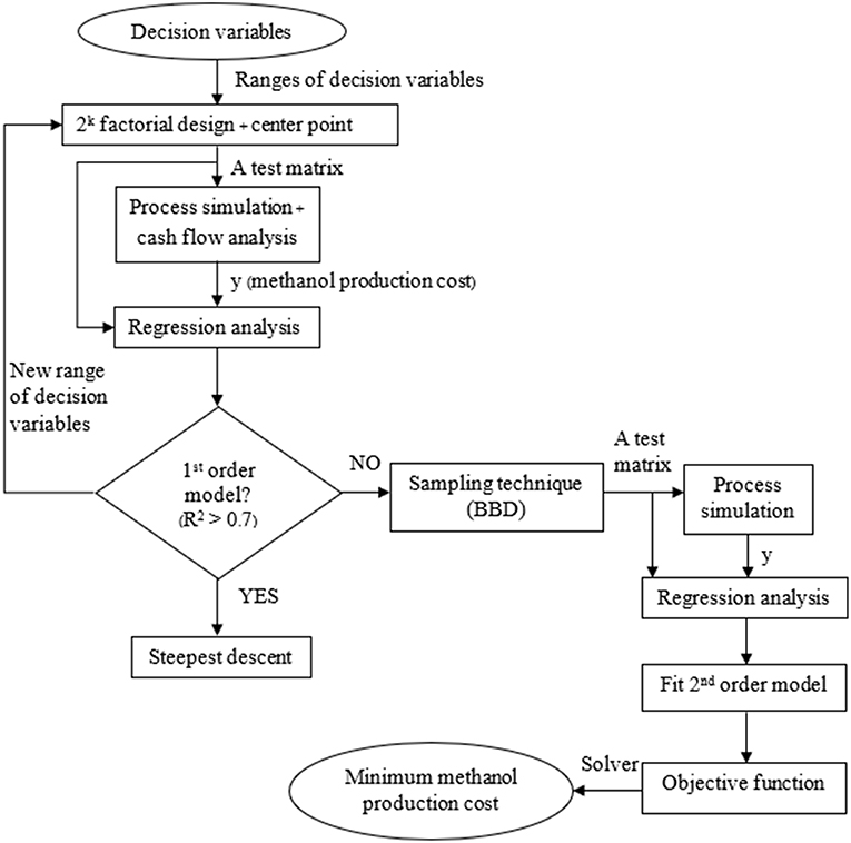
Figure 4. Optimization algorithm.

2^k Factorial Design

The 2^k factorial design is a design for k factors. Each factor is at only two levels, which are values at the lower and upper bounds of the parameter range. The design is generated in coded variables. The coded variable −1 represents the lower bound value, and the coded variable 1 represents the upper bound value. The design is widely used in factor screening experiments. The design observes at each corner of the cube (corner points). Figure 5A demonstrates 2^k factorial design for three independent factors.

FIGURE 5

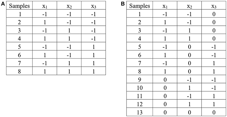
Figure 5. Experimental design: (A) 2^k factorial design for three independent factors, (B) Box – Benhken design for three independent factors.

Steepest Descent

The steepest descent was performed when the data obtained from 2^k factorial design (including one center point) fits the first order model. The steepest descent moves the independent variables to the direction of maximum decrease in the response (Douglas, 2013). To perform the steepest descent, the independent variables will be coded to the (−1, 1) interval as shown in Equation (10). Where x_i is the coded variable, and ξ_i is the natural variable.

$\begin{array}{ll}{x}_i=\frac{{\xi }_i-Midpoint}{\frac{1}{2}Range}& (10)\end{array}$

The regression analysis was performed to fit the data set of 2^k factorial design and a center point with the first order model. Equation (11) represents example of the first order model with five independent factors

$\begin{array}{ll}y=b_0+b_1{x}_1+b_2{x}_2+b_3{x}_3+b_4{x}_4+b_5{x}_5& (11)\end{array}$

A step size (Δx_i) in each independent variable was determined by Equation (12). Where b_{i, highest} is the highest value among all coefficients b_i, except b_o.

$\begin{array}{ll}\Delta x_i=\frac{b_i}{\left|b_{i,highest}\right|}& (12)\end{array}$

The path of steepest descent for x_i was determined by using Equation (13). Where j is point along the path.

$\begin{array}{l}{x}_{i}conditionalongthepath=x_{i,midpoint}+j\Delta x_i\left(\frac{1}{2}Rangeof{x}_i\right);\\ j=1,2,3,\dots & (13)\end{array}$

Experiments were conducted along the path of steepest descent until no further decrease in response.

Box—Behnken Design (BBD)

The Box—Behnken design is the three—level design for fitting response surface (the second order model). The design consists of the midpoint of each edge of the space, and a center point. Figure 5B demonstrates Box—Benhnken design for three independent factors.

Optimization Formulation

This section gives detailed optimization formulation. In the optimization formulation, a second order model was used to represent the response surface. The form of a full second—order model is shown in Equation (14). All five decision variables studied in this work are continuous variables. The decision variables were coded in the ranges between −1 and 1. Therefore, all the constraints are in the boundary of coded variables.

$\begin{array}{ll}\text{MIN}:y={\beta }_0+{\displaystyle \sum _{i=1}^k}{\beta }_i{x}_i+{\displaystyle \sum _{i=1}^k}{\beta }_{ii}{x}_i^2+{\displaystyle \sum }{\displaystyle \sum _{i<j}}{\beta }_{ij}{x}_i{x}_j& (14)\end{array}$

Where y is the methanol production cost ($ per tons produced methanol)

Decision variables:x₁: inlet pressure to the 1st reactor

x₂: inlet temperature to the 1st reactor

x₃: inlet pressure to the 2nd reactor

x₄: outlet temperature of the liquid stream cooler after the 2nd reactor

x₅: inlet temperature to the 1st distillation column

Subject to: −1 ≤ x_i ≤ 1; i = 1, 2, 3, 4, 5

Results and Discussion

We analyzed the impacts of eight operating parameters on the methanol production cost. Then, optimized the value of significant parameters for the minimum methanol production cost. The results obtained from the sensitivity analysis, the steepest descent, and the optimization are discussed in this section.

Simulation—Optimization: Steepest Descent

In performing simulation—optimization algorithm, the first data set (data set 1) from 2^k factorial design with initial range of each decision variable (shown in Table 3, Data set 1 column) was fitted with the first order regression model. The obtained R—squared value is 0.9995. This means the data still fit the linear model. Therefore, we performed steepest descent to search for the region of lower methanol production cost. Figure 6 shows steepest descent in moving the operating conditions to lower methanol production cost region.

TABLE 3

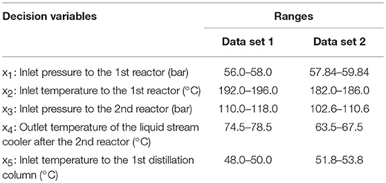
Table 3. Ranges of decision variables.

FIGURE 6

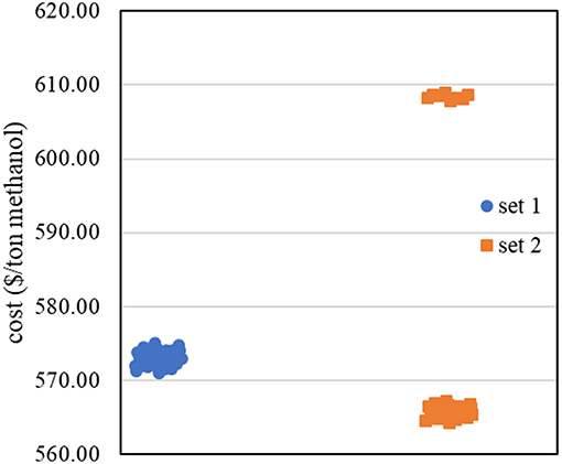
Figure 6. The steepest descent results.

From the steepest descent results, for the first reactor, an increase in inlet pressure from 56.0 to 58.0 bar, and a decrease in inlet temperature from 192.0 to 183.0°C yielded an increase in methanol product at equilibrium condition (%conversion increased from 40 to 45%). For the second reactor, a decrease in inlet pressure from 118.0 to 102.0 bar yielded an increase in methanol product in the reactor. The outlet temperature of the liquid stream cooler after the 2nd reactor decreased from 74°C to around 65°C yielded an increase in liquid methanol separated from the separator. The inlet temperature to the first distillation column increased from 48.0 to 52.0°C yielded higher efficiency to separate most of remaining CO₂ and lighter components from methanol and water.

The steepest descent moves the operating conditions to the new conditions as follows: inlet pressure to the first reactor: 58.84 bar, inlet temperature to the first reactor: 184.0°C, inlet pressure to the second reactor: 106.64 bar, outlet temperature of the liquid stream cooler after the second reactor: 65.54°C, and inlet temperature to the first distillation column 52.75°C. We then used these new operating conditions as the middle value of the range of decision variables. The ranges of the new operating conditions are shown in Table 3, Data set 2 column.

The new data set (Data set 2) was then constructed with 2^k factorial design. The corresponding methanol production costs were collected, as shown in Figure 6. Most of the data in data set 2 shows lower methanol production cost than data set 1, except the data at low inlet pressure to the first reactor. The results agree with the results from sensitivity analysis that the inlet pressure to the first reactor has inversely proportional relationship with the methanol production cost.

By fitting data set 2 with the first—order regression model, the data did not appropriately fit the model as R—squared value is 0.6353 (<0.7). This means that there is high possibility to find the non-linear region at this step. We then used theses ranges of operating condition with BBD in collecting more data for constructing the non-linear model.

The Optimal Conditions

The reduced non-linear model (the model with only significant terms) was constructed with 73 sample points (32 sample points from 2^k factorial design, and 41 sample points from BBD) as shown in Equation (15). The model represents the relationship between the operating conditions and the methanol production cost.

$\begin{array}{ll}y=563.37+7.98x_1-8.22x_2-11.02x_1{x}_2+4.45x_1^2+7.87x_2^2& (15)\end{array}$

Where y is the methanol production cost per tons produced methanol ($ per ton produced methanol), x₁ is inlet pressure to the first reactor, and x₂ is inlet temperature to the first reactor. Please be noted that the obtained values of x₁ and x₂ in Equation (15) are in code variables (−1 to +1). The obtained results have to be converged to the actual operating condition values by using the ranges in Table 3, data set 2 column and Equation (10), where −1 represents the lowest value and +1 represents the highest values in the range.

Table 4 shows the local optimal operating conditions (x_i) of methanol production via CO₂ hydrogenation with the minimum production cost per tons produced methanol (y). Since three parameters, which are inlet pressure to the 2nd reactor (x₃), outlet temperature of the liquid stream cooler after the second reactor (x₄), and inlet temperature to the first distillation column (x₅), do not show significant impacts on the production cost in the non-linear model (Equation 15), the values of these three parameters were set at their lower bounds.

TABLE 4

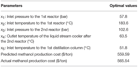
Table 4. The optimal operating conditions obtained from the reduced 2nd order model.

The prediction accuracy of the model was determined by the percent error. The percent error of the model was estimated by comparing between the predicted methanol production cost with the actual production cost. We obtained the actual production cost by running the process simulation with the corresponding optimal operating conditions. The percent error of this non-linear model is 1.05. For regression analysis of this model, the R—squared value is 0.8705, and the adjusted R—squared value is 0.8610. Therefore, with the small number of percent error, it can be concluded that this methanol production via CO₂ hydrogenation process can be represented by the second order model. The process is successfully optimized using RSM.

The optimization formulation was solved in the Intel Pentium 4 processor, core i3. The local optimal solutions were obtained in 2 s. The obtained minimum production cost ($ per tons produced methanol) is an offset between the methanol production cost and the amount of produced methanol. The methanol production cost includes energy consumption, utilities, and capital cost costs. For the optimal solution, the amount of produced methanol increased so that the minimum production cost per tons of produced methanol was obtained. The optimal methanol production rate is 964 kmoles per hours, which produced from 1,000 kmoles per hour of feed carbon dioxide and 3,000 kmoles per hour of feed hydrogen.

Conclusion

In the optimization of methanol production via CO₂ hydrogenation, the sensitivity analysis coupled with RSM was successfully represent the relationship between methanol production operating conditions and the methanol production cost per tons produced methanol ($ per ton produced methanol). The non-linear solver was applied to optimize the non-linear relationship model for the minimum methanol production cost. Two reactors were employed in the process. In the optimal region of study, the inlet pressure and temperature to the first reactor show significant impacts on the methanol production cost. The optimal operating conditions of inlet pressure to the first reactor is 57.8 bar, inlet temperature to the first reactor is 183.6°C, and the other three insignificant parameters were set at their lower bounds. The obtained minimum methanol production cost is $565.54 per ton produced methanol.

Data Availability

All datasets generated and analyzed for this study are included in the manuscript/Supplementary Files.

Author Contributions

PB simulated the process simulation, collected data, analyzed results, and wrote the first draft of the manuscript. AN designed the methodology of the work, and revised the manuscript for the final version.

Funding

Suranaree University of Technology funding on Aspen Hysys simulator.

Conflict of Interest Statement

The authors declare that the research was conducted in the absence of any commercial or financial relationships that could be construed as a potential conflict of interest.

Acknowledgments

The financial support from Suranaree University of Technology is greatly acknowledged.

Supplementary Material

The Supplementary Material for this article can be found online at: https://www.frontiersin.org/articles/10.3389/fenrg.2019.00081/full#supplementary-material

References

Ali, K. A., Abdullah, A. Z., and Mohamed, A. R. (2015). Recent development in catalytic technologies for methanol synthesis from renewable sources: a critical review. Renew. Sustain. Energ. Rev. 44, 508–518. doi: 10.1016/j.rser.2015.01.010

CrossRef Full Text | Google Scholar

Atsonics, K., Panopoulos, K. D., and Kakaras, E. (2015). Thermocatalytic CO₂ hydrogenation for methanol and ethanol production: process improvements. Int. J. Hydrog. Energy 41, 792–806. doi: 10.1016/j.ijhydene.2015.12.001

CrossRef Full Text | Google Scholar

Bukhtiyarova, M., Lunkenbein, T., Kähler, K., and Schlögl, R. (2017). Methanol synthesis from industrial CO₂ sources: a contribution to chemical energy conversion. Catal. Lett. 147:416. doi: 10.1007/s10562-016-1960-x

CrossRef Full Text | Google Scholar

Dasgupta, A., and Klein, K. (2014). “Chapter 5: Oxidative stress induced by household chemicals,” in Antioxidants in Food, Vitamins and Supplements, eds A. Dasgupta and K. Klein (San Diego, CA: Elsevier), 77–95.

Google Scholar

Douglas, C. M. (2013). Design and Analysis of Experiments, 8th Edn. New York, NY: John Wiley & Sons, Inc.

Google Scholar

EPA (2002). US Environmental Protection Agency. Clean Alternative Fuels: Methanol. Technical Report EPA 420-F-00-040. Washington DC, USA: EPA; 2002. Available online at: www.epa.gov.

Google Scholar

Gabele, P. A. (1990). Characterization of emissions from a variable gasoline/methanol fueled car. J. Air Waste Manage. Assoc. 40, 296–304. doi: 10.1080/10473289.1990.10466685

PubMed Abstract | CrossRef Full Text | Google Scholar

Gallucci, F., Paturzo, L., and Basile, A. (2004). An experimental study of CO₂ hydrogenation into methanol involving a zeolite membrane reactor. Chem. Eng. Proc. 43, 1029–36. doi: 10.1016/j.cep.2003.10.005

CrossRef Full Text | Google Scholar

Hoseiny, S., Zare, Z., Mirvakili, A., Setoodeh, P., and Rahimpour, M. R. (2016). Simulation–based optimization of operating parameters for methanol synthesis process: application of response surface methodology for statistical analysis. J. Nat. Gas. Sci. Eng. 34. 439–48. doi: 10.1016/j.jngse.2016.06.075

CrossRef Full Text | Google Scholar

Ingamells, J. C., and Lindquist, R. H. (1975). Methanol as a motor fuel or a gasoline blending component. JSTOR 84, 582–568. doi: 10.4271/750123

CrossRef Full Text | Google Scholar

Jadhav, S. G., Vaidya, P. D., Bhanage, B. M., and Joshi, J. B. (2014). Catalyticcarbon dioxide hydrogenation to methanol: a review of recent studies. Chem Eng Res Design. 92, 2557–2567. doi: 10.1016/j.cherd.2014.03.005

CrossRef Full Text | Google Scholar

Jaworowski, Z., Segalstad, T. V., and Hisdal, V. (1992). Atmospheric CO₂ and Global Warming: A Critical Review, 2nd Edn. Oslo: Norsk Polarinstitutt.

Google Scholar

Jenkins, S. (2018). CEPCI Updates: January 2018 (PRELIM.) and December 2017. Available online at: http://www.chemengonline.com/cepci-updates-january-2018-prelim-and-december-2017-final/?printmode=2011.

Google Scholar

Lachowska, M., and Skrzypek, J. (2004). Methanol synthesis from carbon dioxide and hydrogen over Mn-promoted copper/zinc/zirconia catalysts. React. Kinet. Catal. Lett. 83, 269–273. doi: 10.1023/B:REAC.0000046086.93121.36

CrossRef Full Text | Google Scholar

Leonzio, G. (2017). Optimization through response surface methodology of a reactor producing methanol by the hydrogenation of carbon dioxide. Processes 5:62. doi: 10.3390/pr5040062

CrossRef Full Text | Google Scholar

Liang, X.-L., Dong, X., Lin, G.-D., and Zhang, H.-B. (2009). Carbon nanotube-supported Pd–ZnO catalyst for hydrogenation of CO₂ to methanol. Appl. Catal. B. 88, 315–322. doi: 10.1016/j.apcatb.2008.11.018

CrossRef Full Text | Google Scholar

Machado, C. F. R., Medeiros JLd, O. F. Q., and Araujo, O. F. Q. (2014). “A comparative analysis of methanol production routes: synthesis gas versus CO₂ hydrogenation,” in Proceedings of the 2014 International Conference on Industrial Engineering and Operations Management, Bali, Indonesia.

Google Scholar

María, R. D., Díaz, I., Rodríguez, M., and Sáiz, A. (2013). Industrial methanol from syngas: kinetic study and process simulation. Int. J. Chem. React. Eng. 11, 469–477. doi: 10.1515/ijcre-2013-0061

CrossRef Full Text | Google Scholar

Marlin, D. S., Sarron, E., and Sigurbjörnsson, Ó. (2018). Process advantages of direct CO₂ to methanol synthesis. Front. Chem. 6:446. doi: 10.3389/fchem.2018.00446

PubMed Abstract | CrossRef Full Text | Google Scholar

Naims, H. (2016). Economics of carbon dioxide capture and utilization – a supply and demand perspective. Environ. Sci. Pollut. Res. Int. 23, 22226–22241. doi: 10.1007/s11356-016-6810-2

PubMed Abstract | CrossRef Full Text | Google Scholar

Nuchitprasittichai, A., and Cremaschi, S. (2011). Optimization of CO₂ capture process with aqueous amines using response surface methodology. Comput. Chem. Eng. 35, 1521–1531. doi: 10.1016/j.compchemeng.2011.03.016

CrossRef Full Text | Google Scholar

Radhi, H. (2009). Evaluating the potential impact of global warming on the UAE residentialbuildings – a contribution to reduce the CO₂ emissions. Build. Environ. 44, 2451–2462. doi: 10.1016/j.buildenv.2009.04.006

CrossRef Full Text | Google Scholar

Saito, M., and Murata, K. (2004). Development of high performance Cu/ZnO-based catalysts for methanol synthesis and the water-gas shift reaction. Catal. Surv. Asia 8, 285–294. doi: 10.1007/s10563-004-9119-y

CrossRef Full Text | Google Scholar

Samimi, F., Rahimpour, M. R., and Shariati, A. (2017). Development of an efficient methanol production process for direct CO₂ hydrogenation over a Cu/ZnO/Al₂O₃ catalyst. Catalysts. 7:332. doi: 10.3390/catal7110332

CrossRef Full Text | Google Scholar

Sayah, A. K., Hosseinabadi, S.h, and Farazar, M. (2010). CO₂ abatement by methanol production from flue-gas in methanol plant. World Acad. Sci. Eng. Technol. Int. J. Chem. Molecul. Eng. 4:9. doi: 10.5281/zenodo.1072503

CrossRef Full Text | Google Scholar

Shen, W., Jun, K., and Choi, H. (2000). Thermodynamic investigation of methanol and dimethyl ether synthesis from CO₂ hydrogenation. Kor. J. Chem. Eng. 17, 210–216. doi: 10.1007/BF02707145

CrossRef Full Text | Google Scholar

Sloczyński, J., Grabowski, R., Kozlowska, A., Olszewski, P., Lachowska, M., Skrzypek, J., et al. (2003). Effect of Mg and Mn oxide additions on structural and adsorptive properties of Cu/ZnO/ZrO2 catalysts for the methanol synthesis from CO₂. Appl. Catal. 249, 129–138. doi: 10.1016/S0926-860X(03)00191-1

CrossRef Full Text | Google Scholar

Song, C., Gaffney, A. F., and Fujimoto, K. (2002). CO₂ Conversion and Utilization: an Overview in CO₂ Conversion and Utilization. Washington, DC: American Chemical Society, 2–30.

Google Scholar

Tidona, B., Koppold, C., Bansode, A., Urakawa, A., and Rudolf, V. R. P. (2013). CO₂ hydrogenation to methanol at pressures up to 950 bar. J. Supercrit. Fluid. 78, 70–77. doi: 10.1016/j.supflu.2013.03.027

CrossRef Full Text | Google Scholar

Turton, R., Bailie, R. C., Whiting, W. B., and Shaeiwitz, J. A. (2003). Analysis, Synthesis and Design of Chemical Processes, 2nd Edn. Upper Saddle River, NJ: Prentice Hall.

Google Scholar

Wiesberg, I. L., Medeiros, J. L., Alves, R. M. B., Coutinho, P. L. A., and Araújo, O. Q. F. (2016). Carbon dioxide management by chemical conversion to methanol: Hydrogenation and Bi – reforming. Energy Convers. Manage. 125, 320–335. doi: 10.1016/j.enconman.2016.04.041

CrossRef Full Text | Google Scholar

Witoon, T., Bumrungsalee, S., Chareonpanich, M., and Limtrakul, J. (2015). Effect of hierarchical meso macroporous alumina-supported copper catalyst for methanol synthesis from CO₂ hydrogenation. Energy Conver. Manage. 103, 886–894. doi: 10.1016/j.enconman.2015.07.033

CrossRef Full Text | Google Scholar