Simplification of Data Acquisition in Process Integration Retrofit Studies Based on Uncertainty and Sensitivity Analysis

1. Introduction

The climate change threat is felt more and more as a concern, and countries world wide are nowadays starting to act in order to limit its destructive effects (United Nations, 2015). In this regard, a key role is played by energy efficiency, as its improvement in all human activities is paramount in order to achieve a carbon-neutral economy (The European Commission, 2011, 2014). Concerning industrial processes, Process Integration (PI) methodologies proved to be highly effective in identifying and promoting energy saving possibilities. Potential savings from 10 to 75% have been reported in industrial sectors ranging from petrochemical (Nordman and Berntsson, 2009; Smith et al., 2010; Bütün et al., 2018), to pulp and paper (Ruohonen and Ahtila, 2010), and to food processing (Muster-Slawitsch et al., 2011). PI techniques consist in a collection of methods aiming at the identification of energy recovery opportunities in the industry (see Morar and Agachi, 2010 and Sreepathi and Rangaiah, 2014 for comprehensive reviews). They are characterized by a holistic point of view, focusing on identifying beneficial interconnections among different plant sections and unit operations (Kemp, 2007). External hot and cold utility savings are ultimately achieved by designing (or re-designing) the heat exchangers network and integrating the energy utilities in a better way (e.g., by introducing heat pumps or gas turbines). Since the introduction of the first systematic tool by Linnhoff and Flower (1978) in 1978, known with the name of “Pinch analysis”, many developments have been achieved, (i) extending it to non-energy related targets (e.g., waste-water Wang and Smith, 1994 or emissions minimization and pressure drop optimization Polley et al., 1990), (ii) automating sections of the methodologies by means of computer-aided optimization procedures (Asante and Zhu, 1996; Nie and Zhu, 1999; Smith et al., 2010; Pan et al., 2013; Bütün et al., 2018), and (iii) simplifying the different procedures in order to promote their application in the established industrial practice (Polley and Amidpour, 2000; Dalsgård et al., 2002; Anastasovski, 2014; Pouransari et al., 2014; Chew et al., 2015; Bergamini et al., 2016). These three research lines have often been carried out separately, and in some cases even in a divergent way. The former found a large interest in the ‘80s and early ‘90s (Linnhoff, 1994), and still finds space in the actual research (Klemeš, 2013). It applies the few basic concepts of pinch analysis (such as targeting for minimum consumption) to areas other than energy integration, but still related to energy integration itself. The other two research lines are often divergent in their objectives. They ground on two different philosophies of solving process integration problems: the former striving for the complete automation of the design procedure (possibly relieving the engineer from any design-related decision), the latter believing in the central role of the designer in the decision-making process. For this reason, the recent focus of the first one is in the definition of overarching super-structures for the robust design of heat exchanger networks, while the latter tries to develop heuristics able to easily indicate to the analyst the sub-problems to focus the attention on.

Despite the effort in the development of different approaches, PI methodologies are far from being utilized in the common practice, especially in industrial sectors in which energy costs are not a main concern (e.g., food industry). A primary cause is the requirement of extensive and reliable process data, such as temperatures, mass flow rates and pressures measured before and after all the main process components. This results in a significant time consumption, easily in the order of several weeks, and in a high cost for performing the analysis. Few authors tried to address this issue, recognizing in it a significant (if not the main) barrier for the extensive application of PI techniques. The method proposed by Muller et al. (2007) combines a top-down model relying on linear-regression procedures, to a bottom-up one. The former is used for identifying the main centers of consumption in the plant based on energy bills, while the latter is utilized for modeling the thermodynamic requirements of the previously identified most critical processes. However, despite constituting an interesting approach, it still requires a large amount of data and some extra modeling of sub-processes in order to fit the top-level data. Pouransari et al. (2014) tried to simplify the complexity of PI analysis, by considering the classification of energy data in five different levels of detail. The PI study is then conducted by combining different complexity levels, instead of utilizing a single, detailed one. However, this work does not directly aim at reducing the data acquisition complexity, but rather the successive heat exchanger network design. It proves that not all the data need to be collected at the detailed level, but it does not suggest any criteria for choosing the right level on beforehand. Similar approaches have been discussed mainly for applications of Total Site Analysis, where data acquisition with different levels of detail has been proposed. The generally accepted data classification is between black-box, gray-box, and white-box (Nguyen, 2014). The first considers only utility data, the second adds utility/process interfaces and the third accounts also for process/process interfaces. However, no systematic evaluation for selecting the required detail has been discussed. The work of Kantor et al. (2018) introduced a method for constructing thermal profiles for general industries and industrial sub-processes. It founds on a database of process data from which thermal profiles can be deduced based on top-level data of the studied process (e.g., energy bills, production volumes). It constitutes an interesting attempt of promoting PI techniques, and more development is expected in order to make it a viable tool. Finally, Klemeš and Varbanov (2010) summarized the pitfalls of PI studies, providing some general guidelines for their successful implementation.

This paper presents a novel data acquisition simplification method for PI retrofit studies. It aims at reducing the time consumption (and the cost) of the data acquisition step, by identifying and disregarding the parameters that do not require a precise measurement, before the detailed data acquisition is performed. In this way, it attempts at reducing the existing gap between academic research (often focusing on developing more precise and complex models) and industrial practice (requesting ease of utilization) in the field of Process Integration. Unlike previous studies, the parameters selection is performed in a systematic way, by applying a combination of uncertainty and sensitivity analysis techniques. Uncertainty analysis defines the uncertainty in a model output caused by given uncertainties in the model inputs. Conversely, sensitivity analysis quantifies the individual contribution of input uncertainties to a given output uncertainty (Saltelli et al., 2008). By acknowledging the fact that any analysis is unavoidably prone to uncertainties, no matter the amount of resources dedicated to acquiring refined data, the developed method finds a limited sub-set of data, whose precise measurement suffices for ensuring a selected minimum output uncertainty level. In this context, uncertainty analysis is applied for assessing the output variance and for setting a target for the minimum analysis uncertainty. Sensitivity analysis is employed for solving the “factor fixing” problem, i.e., to identify the input parameters that can be fixed to any roughly estimated value without jeopardizing the output precision (Saltelli et al., 2008). This, in turn, points out the only parameters that require a precise measurement to be collected in the detailed data acquisition phase.

The paper is structured as follows: section 2 presents the basics of the utilized PI technique, the case study, and the novel method developed. The latter is presented in detail, altogether with a description of how it was applied on the case study. Section 3 presents the obtained results, for each step of the proposed procedure. Section 4 discusses merits and pitfalls of the proposed method, providing ideas for future developments. Finally, section 5 presents the conclusions of the study.

2. Methods

This section describes the overall method followed in this study. At first, the common characteristics of process integration techniques are outlined and the case study is introduced. Afterwards, the developed procedure for simplifying and rationalizing the data acquisition step of PI study is presented, altogether with the description of its application on the case study.

2.1. Process Integration Background

Although nowadays PI techniques comprehend numerous different tools, they all ground on the same basic concepts presented by Linnhoff and Hindmarsh (1983). In particular, the very first steps which associate every PI study, regardless of the particular used tool or the type of project (new design or retrofit) comprehend (i) a thorough data acquisition, (ii) an energy targeting, and (iii) a heat exchangers network synthesis (Kemp, 2007).

1. Data acquisition. This is a crucial task, which allows to sort and organize process measurements in order to completely characterize the so called streams. A stream is defined as a flow of matter which is heated or cooled without incurring any variation in its chemical composition. Streams constitute the fundamental units for completely describing the process from an energy point of view. Their characterization generally requires the following steps:

(a) Collect Process measurements. These generally comprehend: (i) temperature, (ii) mass flow rate, (iii) pressure, and (iv) total solids content (in presence of concentration processes) at the inlet and outlet of every process component.

(b) Produce a heat and mass balance for the plant, based on the collected data. This commonly requires the application of data reconciliation techniques.

(c) Extract the streams. After identifying them, every stream should be characterized with (i) supply temperature, (ii) target temperature and (iii) heat capacity rate.

2. Energy targeting. The energy targeting procedure aims at identifying the unavoidable external utilities required by the process calculating, in turn, the maximum potential for internal energy recovery. This is achieved by applying the so called Problem Table Algorithm (PTA) (Linnhoff and Hindmarsh, 1983), which is composed of three main steps:

(a) Subdivide the process in temperature levels based on the supply and target temperatures of the various streams.

(b) Calculate the energy balance in each interval, thus identifying its energy surplus/deficit.

(c) Cascade the energy surplus/deficit to lower temperature levels.

The heat cascade resulting from this procedure provides three main insights in the process: (i) Minimum Hot Utility requirement (HU_min), (ii) Minimum Cold Utility requirement (CU_min), and (iii) Pinch Point temperature (T_pp). These allow confirmation of near-optimal plant designs as such and to rapidly identify improvable layouts providing guidelines for achieving energy savings.

3. Heat Exchangers Network synthesis. In this step the heat exchangers network is designed (in case of grassroot projects) or modified (in case of retrofit projects), in order to reduce the process energy consumption, toward the previously calculated minimum energy targets. No tool exists, which is able to solve this task precisely, easily and in a reasonably fast way in any occasion. As a consequence, this is the stage where most of the developed PI methods differ from one another. The only “red-thread” between most (but not all) of them, can be summarized in the so called “three golden rules” based on the pinch point location: (i) do not heat below the pinch, (ii) do not cool above the pinch, and (iii) do not transfer heat across the pinch.

2.2. Case Study

The investigated case study was a cheese production plant, which constituted a relevant production process for the application of PI techniques. The studied facility was able to process 750 kt/a of raw milk, for producing 75 kt/a of cheese as main product, plus several other by-products among which cream, whey cream and whey proteins. Its energy consumption was subdivided in two energy carriers: (i) electricity, accounting for 35 GWh/a, and (ii) natural gas, accounting for 6.5·10⁶ Nm³/a. A previous study (Bergamini et al., 2016) proved that, by applying PI techniques, a 24% energy consumption reduction could be achieved in an economically feasible manner.

The plant was divided in six sections, namely: (i) weigh in, (ii) milk handling, (iii) culture, (iv) cheese making, (v) normal whey, and (vi) salted whey. They showed a considerable complexity level, employing various interconnected mechanical and thermal unit operations. The most noticeable were heat treatment (e.g., pasteurization and sterilization), filtration and centrifugation units [a more detailed process description is provided in Bergamini et al. (2016)]. The conceptual process layout is shown in Figure 1.

FIGURE 1

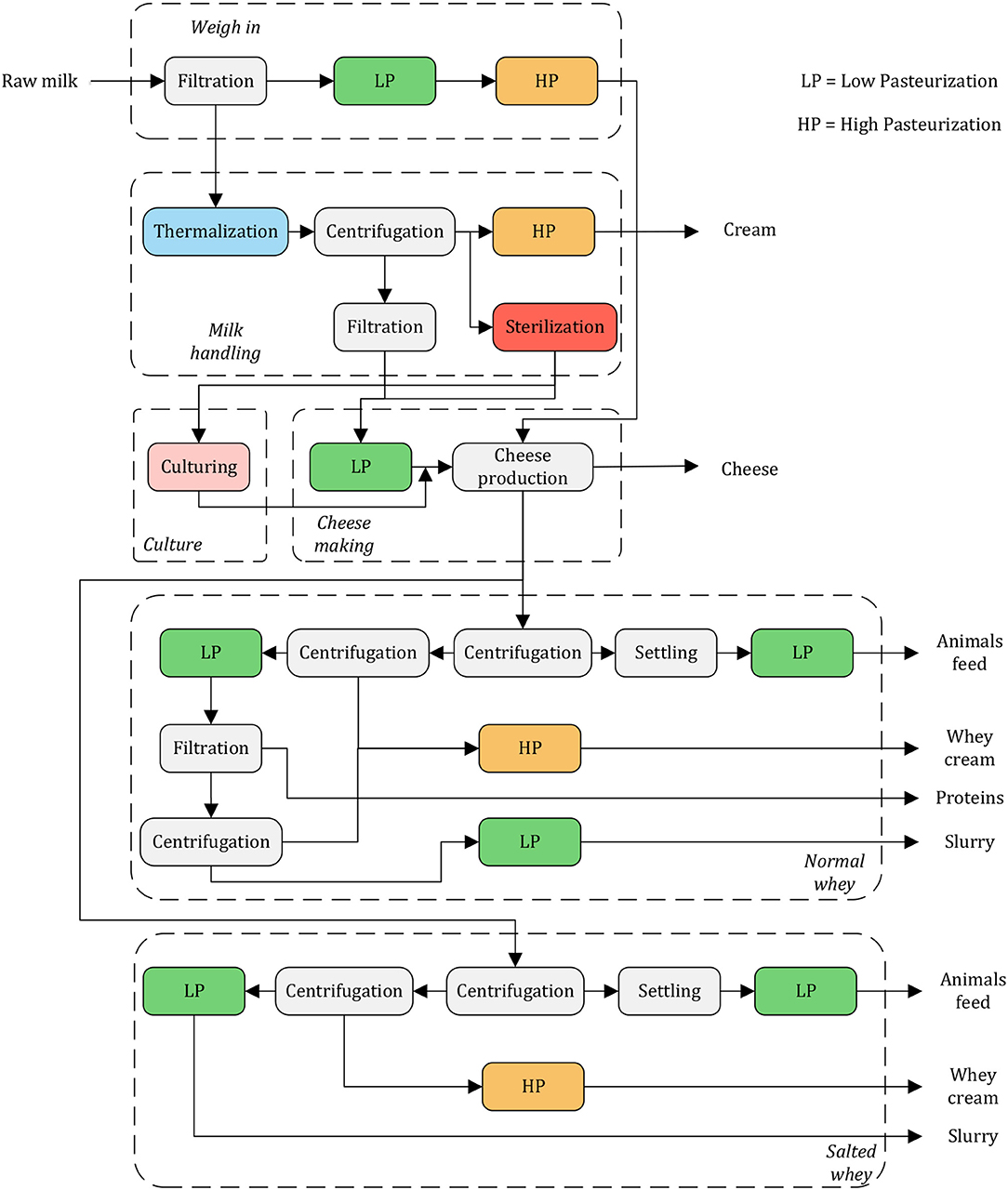
Figure 1. Cheese factory case study conceptual process scheme.

2.3. Data Acquisition Simplification Strategy

Hereby a novel procedure aiming at simplifying the data acquisition step of PI studies is presented. It applies various tools proper to uncertainty and sensitivity analysis, in order to (i) identify non-influencing process parameters, and (ii) determine the maximum acceptable level of uncertainty of the influencing ones. All this is performed before spending time in the detailed data acquisition, in order to conduct such tedious step by targeting a limited set of parameters and knowing the required level of precision in their measurements. The ultimate goal is to minimize the time consumption of the data acquisition process of PI retrofit analysis.

The proposed procedure consists of four consecutive steps (Figure 2). They are explained in detail in the following.

FIGURE 2

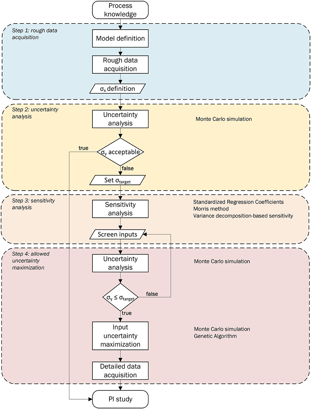
Figure 2. Data acquisition simplification strategy.

2.3.1. Step 1: Rough Data Acquisition

This step constitutes the initialization of the procedure. Starting from process knowledge it results in a first, rough, characterization of the involved parameters. It is composed of two parts:

1. Model definition. At first, a model of the form y = f(x) has to be defined, where x is the vector of the model parameters, f is the model itself, and y is the vector of the model outputs. Considering the specific case of Process Integration studies, the most relevant outputs at a preliminary study level are the energy targets and the pinch point location. The formers quantify the potential savings, while the latter provides information on the possible pathways for reaching them. The model is therefore identified in all the procedures that allow to calculate such outputs based on the process measurements (i.e., the parameters of such model). It is the combination of (i) mass and energy balance, and (ii) Problem Table Algorithm, as summarized in Figure 3.

2. Data acquisition. Once the necessary parameters (i.e., vector x) are identified, they are characterized by assigning estimated values to them, based on information retrieved from e.g., PI diagrams, expert review, process knowledge. At this stage, fast execution is far more valuable than precision. Finally, based on the source of information of individual values, their perceived uncertainty distributions are characterized. As there is no reliable source for such uncertainty definition, overestimation is encouraged, in order to conduct an analysis which is on the “safe side.”

FIGURE 3

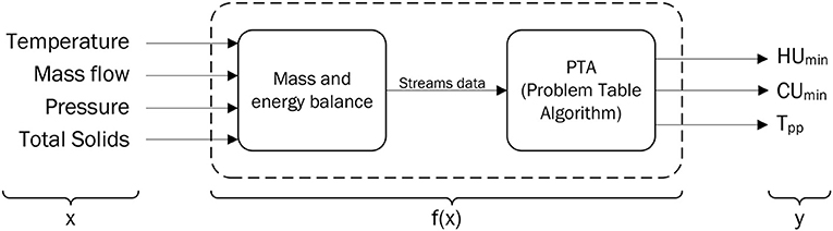
Figure 3. Conceptual model representation.

This procedure was applied on the case study by developing a steady-state mass and energy balance. They were ensured for each individual unit operation, allowing to theoretically deduce some mass flows and temperatures, avoiding their measurements. The total solids content, on the other hand, was assumed based on the nature of the involved material flows (Appendix B). The plant model proved an overall necessity of 205 process parameters values, distributed in 33 mass flow rates, 104 temperatures, 62 total solids contents and 6 energy flows. This data, referred to as nominal values, were acquired from available on-site measurements, expert reviews and annual production and consumption records.

2.3.2. Step 2: Uncertainty Analysis

A first uncertainty analysis is performed on the aforementioned model, aiming at identifying the output uncertainties resulting from the rough data acquisition. In the unlikely event that these uncertainties are considered to be acceptable, there is no need for more precise process data and the PI study can proceed. Otherwise, a maximum output uncertainty threshold (i.e., output standard deviation threshold σ_thresholdj) is defined for each output j, and the following steps are performed in order to ensure that this requirement is met.

Among the possible available techniques (e.g., non-linear regression, bootstrap method, Metropolis algorithm) Monte Carlo analysis (Metropolis and Ulam, 1949) was employed in the present study. This method was preferred for the precision, the ease of implementation and the useful characteristic that the results can be used both for uncertainty propagation assessment and for sensitivity characterization by means of multivariate linear regression techniques. It was performed in three steps (Sin et al., 2009): (i) input uncertainties specification, (ii) input uncertainties sampling, and (iii) propagation of input uncertainties to the model outputs to predict its uncertainties.

1. Step 1. The uncertain parameters were identified and their respective uncertainty was characterized. As data available at this stage derived from rough estimates, no precise identification of the uncertainties was possible directly from the data. The parameters were assumed to be normally distributed, centered on the respective nominal values, according to the recommendations of Madron (1992). The standard deviations were defined in either absolute terms (for temperatures and total solids content) or relative to the nominal values (for mass flow rates and heat flows). Due to the low reliability of the data sources, large standard deviations were assumed (Table 1).

2. Step 2. A sampling number (N = 5, 000) was defined, and an [N-by-k] matrix X was generated by means of Latin hypercube sampling. This was preferred among the other commonly used techniques (e.g., random sampling and Quasi-Monte Carlo sampling) for the good representation of the probability space achieved in a reasonably fast computational time.

3. Step 3. The uncertainties were propagated to the outputs through the model, by performing N simulations using matrix X created in Step 2.

TABLE 1

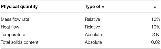
Table 1. Nominal uncertainty definition.

The calculated results could then be used for approximating the output variance by means of simple statistics. As in practice a finite N = 5, 000 was used, the mean and variance estimation by means of Monte Carlo techniques produced an error, which was estimated as (Sin and Gernaey, 2016):

$\begin{array}{ll}{\text{MC}}_{\text{err}}=\frac{{\sigma }_y}{\sqrt{N}}& (1)\end{array}$

where σ_y is the standard deviation of output y.

Finally, based on the results of this analysis, an output uncertainty target was set on the sole HU_min and CU_min. Their target standard deviation was chosen to be 15 and 25% of their nominal value (i.e., the result of the PTA with negligible input uncertainty) respectively, resulting in a value of 346 kW for HU_min and 232 kW for CU_min. Considering the lower importance of T_pp in retrofit studies if compared to the energy targets, as proven by the work of Bonhivers et al. (2017, 2019), it was decided not to set any uncertainty target on T_pp. This might, however, be included in the application of the method. A further discussion is presented in section 4.2 and results obtained setting an uncertainty target on T_pp are presented in Appendix A.

2.3.3. Step 3: Sensitivity Analysis

A sensitivity analysis is performed on the model, in order to solve the “factor fixing” problem. One or several sensitivity methods can be applied. Global sensitivity techniques (e.g., multivariate linear regression, variance decomposition-based sensitivity methods) should be preferred over local ones (e.g., derivative-based methods; Saltelli et al., 2019), as they describe the overall factors influence throughout the totality of their uncertainty domain and considering mutual relations between them. Once the sensitivity measures with respect to all the outputs are calculated, a threshold is defined in order to identify non-influencing parameters and fix them to their nominal values.

In the present study, three different global (or quasi-global) sensitivity analysis techniques were applied, namely: (i) Standardized Regression Coefficients (SRC), (ii) Morris method (MM), and (iii) Variance decomposition-based sensitivity analysis (VDSA).

2.3.3.1. Standardized regression coefficients (SRC)

The standardized regression coefficients quantify the quasi-global sensitivity of the model outputs on input parameters in case of a fairly linearizable model. They were calculated by constructing a linear model based on the output of the Monte Carlo simulation (section 2.3.2). Considering y as the single-valued N-dimensional output vector of the analysis, where N is the sample size, and X the [N-by-k] parameters matrix, a linear regression model was built applying the mean-centered sigma-scaling as Santner et al. (2014):

$\begin{array}{ll}\frac{y_i-{\mu }_y}{{\sigma }_y}={\displaystyle \sum _{j=1}^k}{\beta }_j\frac{X_{i,j}-{\mu }_{X_j}}{{\sigma }_{X_j}}\text{for }i=1,2,\dots ,N& (2)\end{array}$

where β_j is called the Standardized Regression Coefficient (SRC) of parameter j. If the regression is effective (i.e., the model coefficient of determination R² is higher than, 0.7 Sin et al., 2009), the absolute value of β_j can be used to quantify the sensitivity of the output on the various parameters. In fact, R² indicates the fraction of the variance of the original model outputs that is captured by the linear model, and $\sum {({\beta }_j)}^2=R^2$ (Saltelli et al., 2008).

2.3.3.2. Morris method (MM)

The Morris method aims at achieving a quick pre-screening of the influencing parameters, rather than a complete explanation of the output variance, by identifying parameters whose effect is (i) negligible, (ii) linear and additive, or (iii) non-linear or involved in interactions with other parameters. The core of the analysis resides in the definition of the elementary effect attributable to each input. The method was applied by means of the following steps:

1. Step 1. A k-dimensional p-level grid Ω was defined, so that the k-dimensional parameter vector X could take values {0 ≤ X_i ≤ p − 1}. A number of levels p = 8 was considered.

2. Step 2. Each realization of X_i was then transformed in the model input space:

$\begin{array}{ll}{x}_i=A_i+X_i\frac{C_i-A_i}{p-1}& (3)\end{array}$

Where A_i is the lower bound and C_i is the upper bound of parameter i. The lower and upper bounds for all the parameters were set equal to ±3σ, where σ was the one defined in Table 1.

3. Step 3. Selecting a finite perturbation Δ among the multiples of 1/(p − 1), the elementary effect of parameter i was calculated as (Morris, 1991):

$\begin{array}{ll}{\text{EE}}_i(x)=\frac{f(x_1,x_2,\dots ,x_{i-1},x_i+\Delta ,x_{i+1},\dots ,x_k)}{\Delta }& (4)\end{array}$

A general calculation strategy for computing the EE_i in a computationally effective way is presented in Morris (1991) and Campolongo and Saltelli (1997). For easing their confrontation, the elementary effects were standardized by means of standard deviation as proposed by Sin et al. (2009), resulting in the Standardized Elementary Effects (SEE):

$\begin{array}{ll}{\text{SEE}}_i(x)={\text{EE}}_i(x)\frac{{\sigma }_{x_i}}{{\sigma }_y}& (5)\end{array}$

Where σ_xi and σ_y are the standard deviations of the parameter i and the output respectively.

The sensitivity assessment was based on the evaluation of the finite distribution F_i of r elementary effects for each model parameter. At first, a number of repetitions r = 30 was selected. This was repeatedly increased until a stable screening was achieved between different analyses (Ruano et al., 2011). The final accepted number of repetitions was r = 1, 000. A large absolute mean of F_i (μ_{SEE, i}) indicates a large “overall” impact of parameter i on the output, while a significant standard deviation of F_i (σ_{SEE, i}) reveals that the effect of parameter i is highly dependent on the values of the other parameters, i.e., it is non-linear or involved in interactions with other parameters. Finally, the mean of the absolute standardized elementary effects (${\mu }_{\mathrm{\text{SEE}},i}^{*}=\mu (\left|{\mathrm{\text{SEE}}}_i\right|)$) was computed as suggested by Campolongo et al. (2007). It is a good proxy of the previously presented β² and of the total sensitivity index (S_T) introduced in the next sub-section.

2.3.3.3. Variance decomposition-based sensitivity measure (VDSA)

Variance decomposition-based sensitivity measures quantify the influence of input uncertainties on the output variance decomposing it, de facto, in an additive series of terms dependent on the individual uncertainty contributions. Grounding on the works of Hoeffding (1948) and Sobol (1993), the output variance of any model can be completely characterized by 2^k orthogonal summands of different dimensions ${\sigma }_{i_1\dots i_s}^2$. The 2^k sensitivity estimates are then defined as:

$\begin{array}{ll}{S}_{i_1\dots i_s}=\frac{{\sigma }_{i_1\dots i_s}^2}{{\sigma }^2}& (6)\end{array}$

with the convenient property that ∑S_i1…is = 1. The S_i1…is terms constitute a quantitative global sensitivity measure, as they represent the fraction of the output variance caused by individual parameters or the interaction between them. Due to the prohibitively high number of computations for quantifying such terms, they were not calculated in the present work. As more commonly performed, only two groups of indexes were considered, which provide a fairly complete description of the model in terms of its global sensitivity analysis properties:

1. First order effect index S_i. These are the k first order effects, i.e., they quantify the fraction of output variance caused by the individual parameters alone. By doing so, this group of indexes is commonly used for factor prioritization, as it identifies the factors which, if fixed to their true value, result in the highest reduction in output variance.

2. Total effect index S_Ti. They measure the overall effect, i.e., the first and higher effects (interaction effects), of parameters x_i. This group of indexes is commonly used for factor fixing, as it identifies the output variance that would be left if all parameters but x_i, would be fixed to their true values. It follows, that a negligible S_Ti means that the parameter x_i has an overall negligible influence on the output variance. In this way, they eliminate the necessity of computing all the higher order effects.

According to the best practice for computing S_i and S_Ti, two independent [N-by-k] sampling matrices A and B were defined, where N is the number of simulations and k is the number of parameters. By considering these two matrices, other k matrices $A_B^{(i)}$ were computed, where all columns were from A except for the i-th column which was taken from B. By means of these, the sensitivity indexes could be computed according to Saltelli et al. (2009). The computation cost of the analysis was N(k + 2) evaluations of f(x). The method was applied by setting a number of simulations N = 80, 000. This high value was chosen in order to ensure precise estimations for the sensitivity indexes (in particular to ensure S_i ≥ 0).

After applying the three different sensitivity methods, the parameters selected for the subsequent uncertainty maximization step were chosen among the ones identified based on their impact on the sole HU_min and CU_min. Different screening criteria were utilized for the evaluated methods:

• Standardized regression coefficients. Disregard all the parameters with β² ≤ 0.01, i.e., which contribute to <1% to the output variance.

• Morris method. Disregard all the parameters for which both the conditions in Equation (7), Morris (1991), and Equation (8) are verified.

$\begin{array}{ll}{\mu }_{\text{SEE}}\le \frac{{\sigma }_{\text{SEE}}}{\sqrt{r}}& (7)\end{array}$

$\begin{array}{ll}{\mu }_{\text{SEE}}^{*}\le 0.1·\text{max}({\mu }_{\text{SEE}}^{*})& (8)\end{array}$

where $\mathrm{\text{max}}({\mu }_{\mathrm{\text{SEE}}}^{*})$ is the maximum among the mean absolute standardized elementary effect for all the parameters.

• Variance decomposition-based sensitivity. Disregard all the parameters with S_T ≤ 0.01, i.e., which contribute to <1% to the output variance, similarly to β².

The 0.01 threshold was set by defining that such value is close enough to 0, for determining non-influential factors (Saltelli et al., 2008). The threshold expressed in Equation (7) is commonly found in the literature (Morris, 1991), while the one of Equation (8) was arbitrarily set in this work.

2.3.4. Step 4: Allowed Uncertainty Maximization

This step aims at identifying the maximum acceptable uncertainty in the selected parameters, in order to have an uncertainty in the results which does not exceed the threshold set in Step 2. Ultimately, this serves as an indication of the level of precision required for the data acquired during the subsequent “Detailed data acquisition.”

For solving this maximization problem, two tasks are crucial: (i) the definition of the parameters lower and upper bounds and (ii) the selection of the k manipulated parameters.

1. Definition of A_i and C_i. The upper bound (C_i) is trivially set to the initial parameter standard deviation, having no interest in retrieving less precise data with respect to what is already possessed. The definition of the lower bound (A_i), on the other hand, is not as easy. It strongly depends on the process variability, the available measurement system and, ultimately, on measurement costs. Process knowledge and experience are required for completing this task. It is recommended to overestimate this parameter, in order to keep a safety margin.

2. Selection of k manipulated parameters. The manipulated parameters are selected according to the screening conducted in Step 3. However, this does not ensure that the required σ_thresholdj can be achieved with the chosen set of parameters, for their chosen boundaries. In order to verify that this possibility exists, the uncertainty analysis (Step 2) is repeated by setting the standard deviation of the chosen parameters to their lower bounds. If the resulting output uncertainty exceeds the chosen threshold, select a larger set among the screened parameters and repeat this check, until a feasible solution is found. It is recommended to increase the set size gradually, by favoring the intersections between different sensitivity methods results at first, if need be moving toward their union. If necessary, one should consider decreasing the screening thresholds set in Step 3.

This maximization problem is readily expressible as a minimization problem (more easily handled by optimization software) by considering the minimization of the percentage standard deviation reduction (σ_{x, %}) with respect to the nominal value.

$\begin{array}{ll}{\sigma }_{x_i,\%}=\frac{{\sigma }_{x_i}-{\sigma }_{x_i,\text{opt}}}{{\sigma }_{x_i}}& (9)\end{array}$

σ_{xi, opt} represents the standard deviation of the parameter i in the optimized solution.

As multiple parameters are considered, the interest lays in achieving a minimum mean percentage reduction in uncertainty for all the studied parameters (μ(σ_{xi, %})). The task is then to solve the problem specified as:

$\begin{array}{ll}\begin{array}{ll}\underset{x}{\text{min}}\hfill & \mu ({\sigma }_{x_i,\%})\hfill \\ \text{subject to}\hfill & A_i\le {\sigma }_{x_i}\le C_i,\forall i\in 1,2,\mathrm{...},k\hfill \\ \hfill & {\sigma }_{y_j}\le {\sigma }_{{\text{threshold}}_j},\forall j\in 1,2,\mathrm{...},m\hfill \end{array}& (10)\end{array}$

where A_i and C_i are the lower and upper bound of the i-th parameter, while σ_yj and σ_thresholdj are the actual and the threshold standard deviation of the j-th output. Again, σ_yj is calculated by means of uncertainty analysis. This requires running an uncertainty analysis for each set of parameters considered in the optimization procedure, in order to assess the compliance with the boundaries of Equation (10).

In the case study application, the optimization problem was solved by means of the in-built genetic algorithm of Matlab (MAT, 2017), which proved to be superior in terms of minima identification if compared to both the Matlab Particle Swarm Optimizer and Pattern Search, in this particular case. The selected population size was 200 and the number of stalling generations for stopping the algorithm was set to 5. The other options were set to their respective default values. The output uncertainty (σ_yj) was estimated by using the previously utilized Monte Carlo procedure, but this time setting a sample number N = 500 in order to speed-up the computation. In doing so, a larger error on the Monte Carlo estimate, in the order of $\sqrt{10}$, was accepted (Equation 1). This did not affect the final result significantly, as the final error on the uncertainty estimation was below ±5%. The upper bounds for the parameters standard deviation were set equal to the nominal ones, while the lower bounds were set to 25% of the nominal ones. This last choice was roughly taken for sake of proving the method capabilities, but should be better evaluated in a more precise analysis.

3. Results

The results obtained through the application of the proposed method on the case study are presented in the following. They should serve as a demonstration of the method and its use.

3.1. Step 2: Uncertainty Analysis

The uncertainty propagation by means of Monte Carlo simulations resulted, as expected, in large uncertainties on both the energy targets and the pinch point location (Table 2). In particular, σ_CUmin was 63% of μ_CUmin and σ_Tpp was 78% of μ_Tpp.

TABLE 2

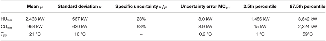
Table 2. Uncertainty analysis results.

This high uncertainty is clearly represented by the Grand Composite Curves (GCC) of the N simulations (Figure 4). Figure 4B shows that the GCC is not a single line (as it would be expected for a PI analysis not accounting for uncertainties), but a family of lines, resulting in a region of possible existence of the points of the GCC, in the T-$\stackrel{\bullet }{Q}$ diagram. Figure 4A shows the approximate probability distribution of all the points composing the GCC. It should be noted that the area comprised in ±3σ (gray area) is very wide, suggesting that an analysis conducted with the present level of data uncertainty would be excessively unreliable. These results formed the basis for setting the aforementioned uncertainty targets (section 2.3.2).

FIGURE 4

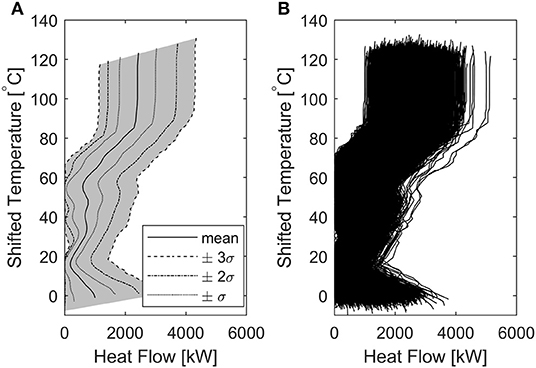
Figure 4. Grand Composite Curve considering uncertainties. (A) approximate probability area for the GCC, (B) aggregated GCC resulting from the N = 5,000 simulations.

3.2. Step 3: Sensitivity Analysis

3.2.1. Standardized Regression Coefficients

Figure 5 shows the Standardized Regression Coefficients analysis results. The graphs on the left side (a, c, e) depict the fit of the linear model for estimating the output variance, to the original output variance as calculated by means of Monte Carlo simulations. Each one of these graphs refers to one of the evaluated model outputs. As should be noted, the linear model fit is good for HU_min and CU_min (graphs a and c), revealing a coefficient of determination (R²) equal to 0.87 and 0.90 respectively. On the other hand, a linear model could not describe the variance of T_pp satisfactorily (graph e), resulting in R² = 0.48, well below the acceptability threshold. This outcome does not surprise, considering the highly non-linear behavior of the pinch point location. It assumes values clustered around few temperature levels, as can be seen in Figure 5E and by inspecting Figure 4A. Focusing next on the β² values depicted in the right hand graphs (b, d, f), for all the evaluated outputs a limited number of parameters demonstrated to be responsible for an appreciable contribution to the output variance for all the outputs, having a β² value above the selected threshold. Moreover, the chosen cut-off threshold for identifying non-influencing parameters proves to be able to detect the rapidly descending trend of β² and the flattening to low values, denoting minor impact of the corresponding model inputs.

FIGURE 5

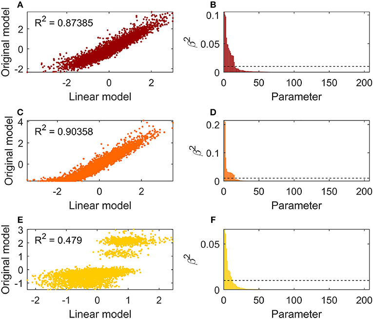
Figure 5. Standardized Regression Coefficients method results of the k = 205 parameters on HU_min (A,B), CU_min (C,D), T_pp (E,F). Figures to the left report the linear model fit to the actual uncertainty. Figures to the right show the β² values of the input parameter sorted in descending order. The dotted lines indicate the proposed cut-off thresholds.

3.2.2. Morris Method

Figure 6 shows the Morris method results. The left hand graphs (a, c, e) depict the mean over the standard deviation relation of the standardized elementary effects distribution of each parameter. The parameters show a horizontal dispersion predominant over the vertical one for HU_min (graph a) and CU_min (graph c), while the opposite is true for T_pp (graph e). This reveals a low non-linear behavior of the input parameters with respect to the energy targets, and a considerable non-linearity concerning the pinch point temperature, confirming the results obtained by the SSC method. Moreover, it can be noted that the majority of the parameters have sensitivity indices located in the region of low importance (low μ_SEE and σ_SEE). Focusing the attention, next, to the right hand graphs (b, d, f) representing the sorted ${\mu }_{\mathrm{\text{SEE}}}^{*}$, it can be noted that, again, a limited number of parameters result in a relevant impact on the output variance. However, unlike the SRC method results, in this case the sorted parameters importance decreases more gradually, resulting in a higher number of parameters deemed influencing.

FIGURE 6

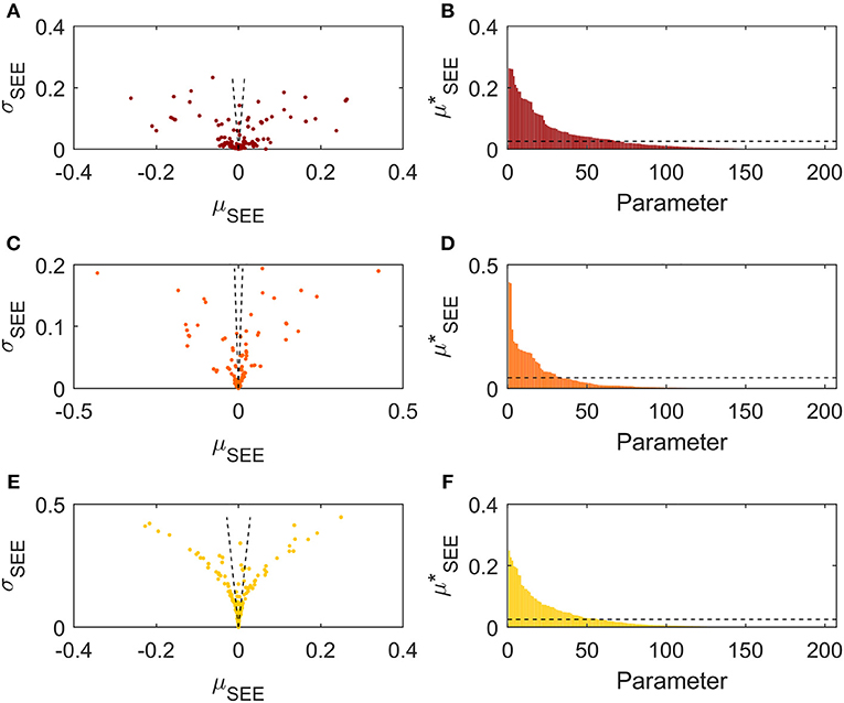
Figure 6. Morris method results of the k = 205 parameters on HU_min (A,B), CU_min (C,D), T_pp (E,F). Figures to the left report the μ_SEE-σ_SEE relations. Figures to the right show the ${\mu }_{\mathrm{\text{SEE}}}^{*}$ values sorted in descending order. The dotted lines indicate the proposed cut-off thresholds.

3.2.3. Variance Decomposition-Based Sensitivity Measure

Figure 7 presents the total sensitivity index of the evaluated parameters with respect to each output, sorted in descending order. As for the previously commented methods, it can be noted that few parameters have a relevant impact on the energy targets (graphs a, b), showing high S_T for a limited number of factors and a steep decrease of this value, which starts to flatten around the 30th parameter. Moreover, the cut-off threshold chosen for identifying non-influencing parameters (showed in dotted lines) proves to be able to detect this flattening region. The same cannot be said of the pinch point location (graph c). In this case the number of parameters influencing the output variance is higher, accounting for 80 factors.

FIGURE 7

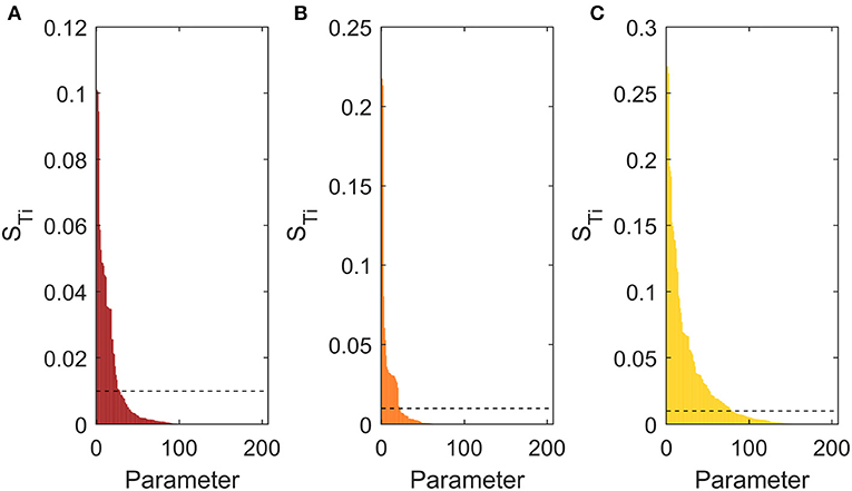
Figure 7. Total sensitivity index of the k = 205 parameters on the outputs, sorted in descending order. (A) Sensitivity on HU_min, (B) Sensitivity on CU_min, (C) Sensitivity on T_pp. Dotted lines indicate the proposed cut-off threshold.

3.2.4. Sensitivity Methods Comparison

The three sensitivity methods were firstly compared based on their ability to detect important and non-important parameters (Figure 8). Specifically, the “total” sensitivity measures were accounted for, namely β², ${\mu }_{SEE}^{*}$ and S_T. No correlation was detected for the sensitivity indices on T_pp (yellow dots) related to the SRC method. This is caused by the poor fit of the linear model to the pinch point uncertainty. On the contrary, a very good correlation was found between the Morris method and the variance decomposition-based sensitivity (Figure 8C). Considering the sensitivity indices on energy targets, all the methods show good agreement in detecting highly influencing parameters, suggesting a low risk of committing type II statistical errors i.e., classification of important parameters as unimportant (Saltelli et al., 2008). Less agreement resulted for low sensitivity measures. In particular, in this region the Morris method tended to overestimate the factors impact compared to both multivariate linear regression and variance decomposition-based techniques (Figures 8A,C). This indicates the risk of committing type I statistical errors, i.e., classification of unimportant parameters as important (Saltelli et al., 2008), when utilizing the Morris method. Much higher agreement was found between SRC and Variance-based decomposition (Figure 8B). They achieve an almost perfect correlation for high sensitivity measures, finding disagreement just at low measures. In particular, the former tends to underestimate the factors importance in this region, if compared to the theoretically more precise VDSA. In general, the better correlation between β² and S_Ti was expected, considering that they both represent the same measure, i.e., the decomposition of the output variance. On the other hand, ${\mu }_{SEE}^{*}$ expresses the normalized average influence of single parameters on the outputs, but it does not explicitly aim at explaining the individual contribution to the output uncertainty.

FIGURE 8

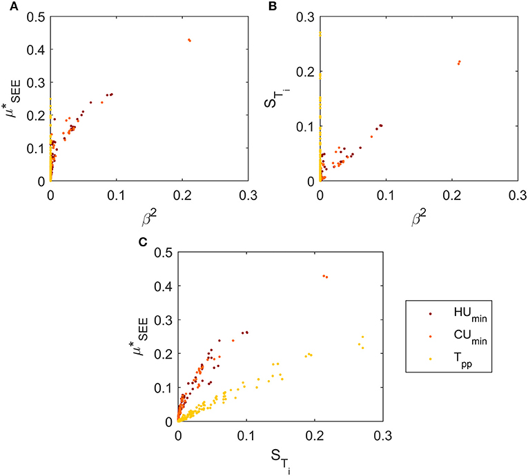
Figure 8. Comparison of sensitivity indices for the k = 205 parameters. (A) β² vs. ${\mu }_{\text{SEE}}^{*}$, (B) β² vs. S_Ti, (C) S_Ti vs. ${\mu }_{\text{SEE}}^{*}$.

As aforementioned, it was decided to focus the analysis on the sole energy targets. Therefore, the parameter screening was performed disregarding the influence on the pinch location. As a result, 28 parameters were selected by the SRC, 52 by the Morris method and 32 by the variance decomposition-based technique. The different results obtained by considering also a target on the pinch location (i.e., adding a maximum threshold of 25% of the nominal T_pp value for T_pp) are presented in Appendix A.

The three sensitivity methods were then compared on the basis of the selection of important parameters (Figure 9).

FIGURE 9

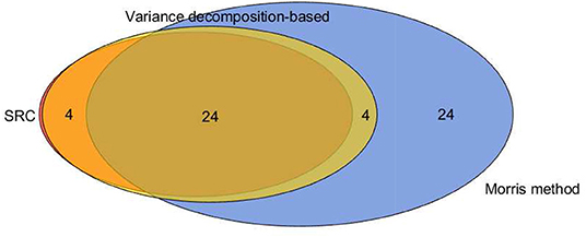
Figure 9. Comparison of the important parameters selected by different sensitivity methods.

SRC and variance decomposition-based techniques showed a good agreement in classifying the important factors. In particular, all the parameters selected by the former were also identified by the latter. Moreover, just 4 factors identified by the VDSA exceeded the ones spotted by SRC. Concerning the Morris method, it selected 24 parameters that do not find agreement with the other sensitivity analysis techniques. This could signify, once again, the risk of committing type I statistical errors when utilizing it for screening. All in all, 24 factors were screened by all the three techniques.

3.3. Step 4: Allowed Uncertainty Maximization

Step 4 of the procedure was conducted for the parameters selected in Step 3 (Figure 9). The ones disregarded in the sensitivity analysis performed were not considered influencing, according to the Factor fixing setting of the study. As three different sensitivity analysis methods were used in this work, three different sets of parameters were selected in Step 3 and a final set to be considered at this stage had to be chosen. At first, the set {SRC∩MM∩VDSA} (composed of 24 parameters) was selected, and the uncertainty analysis by means of Monte Carlo techniques was performed. Unlike step 2 of the procedure, however, this time the uncertainty assigned to the 24 selected factors was set to the lower boundaries previously defined for their measurement. This indicates the very minimum uncertainty achievable by retrieving the most precise data technically possible for the selected parameters. The resulting standard deviation of the energy targets was 347 kW for HU_min and 219 kW for CU_min. The former was slightly higher than the required uncertainty target (i.e., 346 kW, section 2.3.2) and, according to the procedure, a larger parameters sub-set was selected. The set {SRC∩VDSA} composed of 28 parameters resulted in a minimum standard deviation of 254 and 216 kW for HU_min and CU_min respectively, both below the targets. This proved that a detailed data acquisition performed on this set of factors could reduce the output uncertainty below the defined threshold. Therefore, the analysis was continued with this sub-set, and the consideration of a larger one was not necessary.

The required uncertainty reduction for the 28 parameters, presented as percentage reduction with respect to the uncertainty on the rough data, is reported in Figure 10. Just a few parameters need an uncertainty as low as their lower bound (i.e., 75% in the graph), while others need a lower uncertainty reduction. In particular, three factors require a standard deviation reduction of just 10%, indicating that their detailed measurement might not be paramount. Such result indicates that the important parameters might have been over-estimated, while selecting few that were not so important. However, the amount of selected factors is limited, not invalidating the method performance in screening the required measurements.

FIGURE 10

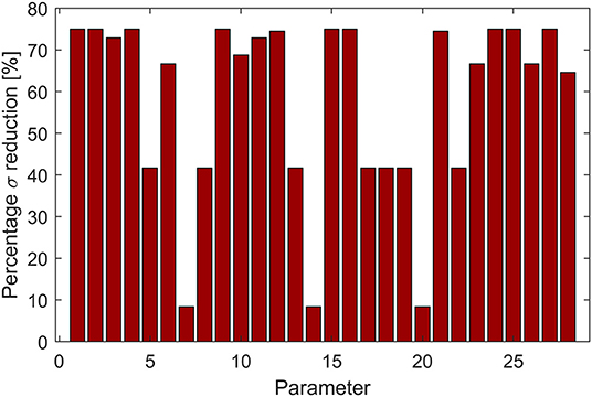
Figure 10. Minimum percentage standard deviation reduction on the selected parameters sub-set required in order to ensure an output uncertainty lower than the targets.

The uncertainty resulting by acquiring detailed measurements complying with the targets for the 28 selected inputs (while keeping the rough estimates for the others, together with their initial large uncertainty) are presented in Figure 11 and Table 3. As it can be noted, the output uncertainty targets were respected, within the Monte Carlo procedure error range, proving that a data collection performed with the indicated uncertainty on the selected sub-set of parameters could satisfy the analyst requirements.

FIGURE 11

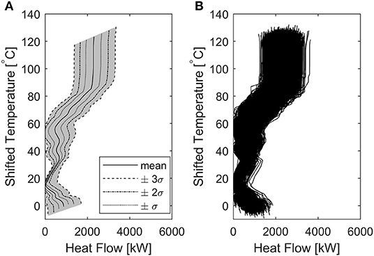
Figure 11. Grand Composite Curve considering reduced uncertainties for the k=28 parameters ({SRC∩VDSA}). (A) probability area for the GCC, (B) aggregated GCC resulting from the N = 5,000 simulations.

TABLE 3

Table 3. Uncertainty analysis results for the reduced input uncertainty on k = 28 parameters ({SRC∩VDSA}).

After assessing that a detailed data acquisition conducted on the selected sub-set of parameters sufficed for reaching the output uncertainty targets, the composition of the chosen sub-set of factors was investigated. It was found that all the 28 parameters were either inlet or outlet temperatures belonging to 18 different streams. No mass flow rate, total solid content, or heat flow was deemed important. The process streams requiring detailed data acquisition were then inspected, in order to assess the reason of their importance. Figure 12 presents the mass flow rate of all the streams identified in the PI study (in total 61), sorted in descending order. Red bars indicate streams requiring detailed acquisition of inlet and/or outlet temperature.

FIGURE 12

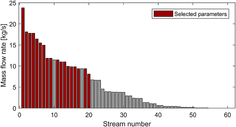
Figure 12. Stream mass flow rates sorted in descending order. Red bars indicate the streams selected for detailed measurement.

As it can be noted, all the streams with higher mass flow rate were selected for further data assessment, with the sole exception of two, indicating a strong relationship between the mass flow rate and the streams importance.

Finally, in order to prove the goodness of the chosen uncertainty thresholds for the study, an uncertainty analysis was conducted by reducing the uncertainty for all the 205 parameters to their lower bound. This represents the lowest possible output uncertainty attainable by performing a detailed data acquisition on all the parameters. The results are presented in Figure 13 and Table 4. As it can be noted by comparing Tables 3, 4, the overall uncertainty on the energy targets achieved by performing the detailed data acquisition on only 28 parameters is not excessively higher than the minimum obtainable one (15% against 7% for HU_min and 27% against 19% for CU_min), especially considering the attained reduction in the number of parameters (28 against 205). The same cannot be claimed for the pinch location, as expected, as it was not a goal to reduce its uncertainty. Similar conclusions can be graphically deduced by comparing Figures 11, 13. All in all, the results indicate the effectiveness of the proposed data acquisition simplification strategy in identifying a limited sub-set of parameters whose precise measurement suffices for attaining a reasonably low uncertainty in the pinch targeting procedure. Once again, it should be kept in mind that if a lower output uncertainty was sought, the respective target could be set at a lower level and a different parameters sub-set could have been identified, in order to meet the targets.

FIGURE 13

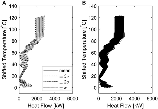
Figure 13. Grand Composite Curve considering minimum uncertainties for the k = 205 parameters. (A) probability area for the GCC, (B) aggregated GCC resulting from the N = 5,000 simulations.

TABLE 4

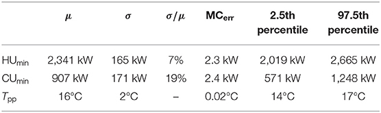
Table 4. Uncertainty analysis results for the minimum possible input uncertainty on k = 205 parameters.

4. Discussion

The results demonstrate that the proposed method was able to effectively reduce the number of data to be retrieved in the detailed data acquisition phase of a PI study, when applied to the case study. The complexity of this step was remarkably reduced compared to the common practice in Process Integration (Kemp, 2007), pointing out that only 28 process parameters over the total 205 needed precise assessment. Moreover, unlike previously developed tools (Muller et al., 2007; Klemeš and Varbanov, 2010; Nguyen, 2014; Pouransari et al., 2014; Kantor et al., 2018), the parameters selection was conducted in a systematic way ground on statistics, and the required precision in the collected values was identified. This information was available before actually performing the measurements, reducing significantly the time dedicated to data acquisition. It can be claimed, therefore, that the application of the proposed data acquisition simplification strategy has the potential of reducing the gap between academia and industry in matter of Process Integration. However, some limitations calling for further developments need to be mentioned and some implications of the obtained results are worth discussing.

4.1. Practical Implications

As the method was applied, three different global sensitivity analysis techniques were employed and compared. This might be unreasonable for an industrial application, for which it might be more appealing to utilize only one of them. This would reduce the time dedicated to the analysis and the complexity in comparing different results. However, the comparison of the methods did not lead to any conclusive remark regarding which method better identifies the influencing parameters. The results are subject to a large extent to the decision of (i) minimum acceptable output uncertainty threshold (Step 2) and (ii) methods cut-off criteria (Step 3). No general recommendation is provided so far on how to best set such thresholds, as such decision is likely to be case-specific and further applications of the method are needed for generalizing any conclusion. However, on the basis of this specific case study, some observations can be made:

1. The SRC and VDSA methods resulted in a similar parameters selection. The four parameters selected just by VDSA did not result to be decisive for meeting the selected output uncertainty targets. However, as this discrepancy is limited, it can be concluded that both methods performed well in screening the most influencing parameters. This agrees with the expectations to achieve good results by applying the SRC (R² was reasonably close to 100%) and to achieve a satisfactory variance decomposition by applying VDSA (Saltelli et al., 2008).

2. The Morris method selected 24 parameters not chosen by the other techniques. As their inclusion proved to be unnecessary for meeting the output uncertainty target, this points out once more the risk of committing type I statistical errors by using MM. This risk has not been discussed in the literature, which on the contrary points out the efficacy of MM (Campolongo and Saltelli, 1997; Campolongo et al., 2007; Ruano et al., 2011). However, the experienced liability is likely to be case specific and especially related to the chosen uncertainty targets and screening thresholds. A proof of this is given in Appendix A, which shows how setting different targets, the screening performed by the Morris method identifies less surplus parameters if compared to VDSA.

3. Considering the computational time involved in the usage of these methods, the SRC proved to be much faster than the other methods in providing the results, as it could be expected. The computational cost was N = 5, 000 function evaluations for SRC, while (k + 1)r = 206, 000 function evaluations were required for the Morris method, and N(k + 2) = 16, 560, 000 function runs were necessary for VDSA. Considering the computational time, this resulted in <5 min compared to about 2 h and to about 90 h, respectively, if run on a single 2.5 GHz processor. If the time for the sensitivity analysis is a concern, it is therefore recommended to just employ the SRC method, as long as the coefficient of determination is higher than 70%, accordingly to what is advised in the literature (Sin et al., 2011). In case the selected parameters sub-set could not meet the maximum allowed output uncertainty, it is possible to increase the parameters cut-off threshold (Step 3). Such iterative procedure would still be faster than the VDSA computation at the price of a little imprecision in the identification of the final parameters sub-set. If on the other hand the coefficient of determination is lower than 70%, the usage of VDSA is advised, as long as the computational time required is deemed reasonable. These recommendations find agreement with the commonly accepted practice (Saltelli et al., 2008, 2009; Sin et al., 2011).

The nature of the finally selected parameters revealed a certain correlation between streams mass flow rate and importance in collecting detailed data measurements (Figure 12). This gives reason to the generally accepted rule of thumb that particular care should be taken in collecting data on the largest streams (Kemp, 2007; Klemeš and Varbanov, 2010; Pouransari et al., 2014; Bergamini et al., 2016). However, the fact that not all the largest streams were deemed important for achieving the uncertainty targets points out the usefulness in having a systematic procedure for determining important measurements, rather than rules of thumb based on the aforementioned observation (most of which generally ground on the 80/20 Pareto principle Ho, 1994). This benefit derived by using the proposed method is even more evident in the application presented in Appendix A.

4.2. Limitations

The proposed method provides large flexibility to the analyst in the definition of (i) data uncertainties and (ii) objectives of the analysis. If on one side this allows for adjusting the procedure to the needs of the specific project under evaluation, on the other hand it requires some experience in order to be applied. The main decisions left to the analyst are discussed in the following.

Arguably, the most important task is the definition of the parameters uncertainties, both on the rough data estimates (Step 1) and for setting the lower bounds for the optimization (Step 4). Different issues arise: (i) as the rough data acquisition mostly makes use of opinions and design set points, no hard proof is available to base the uncertainties estimate on. It is therefore important to stay on the safe side at this stage and assign large uncertainties. (ii) Freedom exists in setting the parameters uncertainties lower bound, as they are related, among other factors, to the utilized measurement instrumentation. Respecting the boundaries set by available measurement systems, a major role in this choice is played by the cost of reaching a given uncertainty level (e.g., for buying more precise instruments or making use of multiple measurement points). This aspect was not considered in this study. The development of rules of thumb would be beneficial for helping the practitioner in successfully handling the proposed procedure.

The choice of the objective function in Step 4 of the procedure (Equation 10) could be open to discussion. In this paper it is suggested to minimize the average uncertainty reduction on the parameters to be measured, provided that the choice of the parameters is already made. Clearly, there could be other possibilities, e.g., minimize the number of parameters to be measured, provided that their uncertainty is reduced to their lower bound. We decided to prefer the first one, recognizing that the complexity in performing measurements is not only determined by the number of parameters to be measured, but also by the required precision of their measurements (which defines, e.g., the number of samples and sampling points). With these two aspects in mind, the parameters selection is performed solely in Step 3 (sensitivity analysis) and the uncertainty reduction minimization in Step 4. Again, the key for determining the best possible objective function is to be found in cost evaluations, i.e., in assessing whether it is less expensive to collect less accurate but more numerous data, or to acquire more precise but less numerous measurements.

The analyst is empowered to decide the outputs to be considered as relevant for the analysis he wants to perform. As an example, in the application presented in this study it was decided to disregard the pinch point location as a relevant output of the problem table algorithm in case of retrofit projects. This was based on the recognition that the knowledge of the global T_pp is not fundamental for achieving energy savings in existing plants, as proved by the work of Bonhivers et al. (2017, 2019). The Bridge analysis method they proposed demonstrated that removing heat transfer across the global pinch is not necessary to save energy. However, one might want to determine T_pp precisely, as its knowledge is important for employing more traditional PI retrofit methods (Tjoe and Linnhoff, 1986; Nordman and Berntsson, 2001). A target for the maximum allowable uncertainty on the pinch point location could be set with no harm, as demonstrated in Appendix A. Clearly, this choice affects the method results and has to be considered carefully.

4.3. Future Work

Further development of the procedure for providing criteria able to help the analyst in taking these decisions would be beneficial. This requires: (i) additional testing of the method on different case studies, (ii) the impact assessment of the rough assumptions made on the uncertainties distributions, and (iii) to include considerations of costs related to conducting measurement campaigns. This last aspect has not been considered so far in the Process Integration literature, and its consideration would help to further bridge academic development and industrial practice.

Another interesting development would be in extending the application of this method to energy analysis other than PI techniques (e.g., energy auditing, energy analysis). As it is proposed in this work, the developed procedure is generally applicable to any PI retrofit study for addressing the data acquisition phase, no matter the method utilized for the heat exchangers network design. In fact, all the available synthesis techniques can benefit of a wisely conducted data collection able to reduce the time consumption, and the related costs, of the project. However, the proposed logic of combining uncertainty and sensitivity analysis techniques for determining the necessary measurements has the potential of being generally applied to any energy analysis, provided that the considered model (Figure 3) and the analysis outcomes (i.e., energy targets and pinch location) are different than the ones presented for PI techniques in this paper. This could also serve as a rational criterion for selecting required measurement points in the installation of a permanent measurement system able to assess the process energy performance. Again, further testing in different case studies and for different types of analysis is needed to verify this argumentation.

5. Conclusion

A novel method aiming at reducing the time consumption (and cost) in the data acquisition step of process integration retrofit studies was presented. It systematically employs a combination of uncertainty and sensitivity analysis techniques in order to solve the “factor fixing problem” and identify a sub-set of process parameters that need precise measurements for conducting the project. This feature lowers one of the main barriers for the application of PI techniques in the common industrial practice, i.e., the significant time dedicated to tedious process data acquisition. From its application on a dairy process the following can be inferred:

• The method was shown to be able to: (i) calculate the uncertainty on the problem table algorithm outputs and set a target for the maximum allowable uncertainty, (ii) identify the sub-set of most influencing process values required for performing the process integration analysis, and (iii) determine the maximum acceptable uncertainty on this sub-set of process data in order to reach the required output uncertainty. All these results are made available before conducting the detailed data acquisition. The method recommended to collect detailed measurements on only 28 parameters out of the total 205 required by existing PI procedures, resulting in significant time savings in this operation.

• The procedure is flexible in defining screening criteria and output uncertainty targets, leaving the analyst freedom to adjust the screening to case-specific analysis requirements.

• Different global sensitivity analysis methods can be used in the simplification procedure. The required computational time suggests to employ multivariate linear regression on Monte Carlo results as first attempt, moving to Morris method or variance decomposition-based analysis in case of bad fitting of this one.

• The experience of the analyst is particularly needed in defining the uncertainties on the input data before performing measurements. Further study is required in order to develop guidelines for performing this task.

Overall it can be concluded that the developed method has the potential to reduce the gap between academic research and industrial needs in matter of process integration, promoting the usage of such techniques in the industrial practice.

Author Contributions

RB, T-VN, and BE contributed in the conception and design of the study. RB conceived the method and performed the case study analysis. T-VN and BE provided guidance and inputs in the method criteria definition and critically revised the method. All authors contributed to manuscript revision, read, and approved the submitted version.

Conflict of Interest

The authors declare that the research was conducted in the absence of any commercial or financial relationships that could be construed as a potential conflict of interest.

Supplementary Material

The Supplementary Material for this article can be found online at: https://www.frontiersin.org/articles/10.3389/fenrg.2019.00108/full#supplementary-material

References

Anastasovski, A. (2014). Enthalpy table algorithm for design of heat exchanger network as optimal solution in Pinch technology. Appl. Thermal Eng. 73, 1113–1128. doi: 10.1016/j.applthermaleng.2014.08.069

CrossRef Full Text | Google Scholar

Asante, N. D., and Zhu, X. X. (1996). An automated approach for heat exchanger network retrofit featuring minimal topology modifications. Comput. Chem. Eng. 20, 7–12. doi: 10.1016/0098-1354(96)00013-0

CrossRef Full Text | Google Scholar

Bergamini, R., Nguyen, T.-V., Bühler, F., and Elmegaard, B. (2016). “Development of a simplified process integration methodology for application in medium-size industries,” in Proceedings of ECOS 2016–the 29th International Conference on Efficiency, Cost, Optimization, Simulation and Environmental Impact of Energy Systems (Portorož).

Google Scholar

Bonhivers, J. C., Moussavi, A., Hackl, R., Sorin, M., and Stuart, P. R. (2019). Improving the network pinch approach for heat exchanger network retrofit with bridge analysis. Can. J. Chem. Eng. 97, 687–696. doi: 10.1002/cjce.23422

CrossRef Full Text | Google Scholar

Bonhivers, J. C., Srinivasan, B., and Stuart, P. R. (2017). New analysis method to reduce the industrial energy requirements by heat-exchanger network retrofit: Part 1 – Concepts. Appl. Therm. Eng. 119, 659–669. doi: 10.1016/j.applthermaleng.2014.04.078

CrossRef Full Text | Google Scholar

Bütün, H., Kantor, I., and Maréchal, F. (2018). A heat integration method with multiple heat exchange interfaces. Energy 152, 476–488. doi: 10.1016/j.energy.2018.03.114

CrossRef Full Text | Google Scholar

Campolongo, F., Cariboni, J., and Saltelli, A. (2007). An effective screening design for sensitivity analysis of large models. Environ. Model. Softw. 22, 1509–1518. doi: 10.1016/j.envsoft.2006.10.004

CrossRef Full Text | Google Scholar

Campolongo, F., and Saltelli, A. (1997). Sensitivity analysis of an environmental model: an application of different analysis methods. Reliabil. Eng. Syst. Safety 57, 49–69. doi: 10.1016/S0951-8320(97)00021-5

CrossRef Full Text | Google Scholar

Chew, K. H., Klemeš, J. J., Alwi, S. R. W., and Manan, Z. A. (2015). Process modifications to maximise energy savings in total site heat integration. Appl. Therm. Eng. 78, 731–739. doi: 10.1016/j.applthermaleng.2014.04.044

CrossRef Full Text | Google Scholar

Dalsgård, H., Petersen, P. M., and Qvale, B. (2002). Simplification of process integration studies in intermediate size industries. Energy Convers. Manage. 43, 1393–1405. doi: 10.1016/S0196-8904(02)00023-7

CrossRef Full Text | Google Scholar

Ho, Y.-C. (1994). Heuristics, rules of thumb, and the 80/20 proposition. IEEE Trans. Autom. Control 39, 1025–1027.

Google Scholar

Hoeffding, W. (1948). A class of statistics with asymptotically normal distribution. Ann. Math. Stat. 19, 295–325.

Google Scholar

Kantor, I., Santecchia, A., Wallerand, A. S., Kermani, M., Salame, S., Arias, S., et al. (2018). “Thermal profile construction for energy-intensive industrial sectors,” in Proceedings of ECOS–The 31st International Conference on Efficiency, Cost, Optimization, Simulation and Environmental Impact of Energy Systems (Guimaraes).

Google Scholar

Kemp, I. C. (2007). Pinch Analysis and Process Integration: A User Guide on Process Integration for the Efficient Use of Energy, 2 Edn. Burlington, VT: Butterworth-Heinemann.

Google Scholar

Klemeš, J., and Varbanov, P. (2010). Implementation and pitfalls of process integration. Chem. Eng. Trans. 21, 1369–1374. doi: 10.3303/CET1021229

CrossRef Full Text | Google Scholar

Klemeš, J. J. (2013). Handbook of Process Integration (PI): Minimisation of Energy and Water Use, Waste and Emissions, 1st Edn. Cambridge: Woodhead Publishing Limited.

Google Scholar

Linnhoff, B. (1994). Use pinch analysis to knock down capital costs and emissions. Chem. Eng. Progress 18, 32–57.

Google Scholar

Linnhoff, B., and Flower, J. R. (1978). Synthesis of heat exchanger networks: I. Systematic generation of energy optimal networks. AIChE J. 24, 633–642.

Google Scholar

Linnhoff, B., and Hindmarsh, E. (1983). The pinch design method for heat exchanger networks. Chem. Eng. Sci. 38, 745–763.

Google Scholar

Madron, F. (1992). Process Plant Performance: Measurement and Data Processing for Optimization and Retrofit. Chichester: Ellis Horwood Limited Co.

Google Scholar

MATLAB Release R2017b (2017). MATLAB Release R2017b. Natick, MA: The MathWorks Inc.

Google Scholar

Metropolis, N., and Ulam, S. (1949). The Monte Carlo Method. J. Am. Stat. Assoc. 44, 335–341.

PubMed Abstract | Google Scholar

Morar, M., and Agachi, P. S. (2010). Review: Important contributions in development and improvement of the heat integration techniques. Comput. Chem. Eng. 34, 1171–1179. doi: 10.1016/j.compchemeng.2010.02.038

CrossRef Full Text | Google Scholar

Morris, M. D. (1991). Factorial sampling plans for preliminary computational experiments. Technometrics 33, 161–174.

Google Scholar

Muller, D. C. A., Marechal, F. M. A., Wolewinski, T., and Roux, P. J. (2007). An energy management method for the food industry. Appl. Therm. Eng. 27, 2677–2686. doi: 10.1016/j.applthermaleng.2007.06.005

CrossRef Full Text | Google Scholar

Muster-Slawitsch, B., Weiss, W., Schnitzer, H., and Brunner, C. (2011). The green brewery concept - energy efficiency and the use of renewable energy sources in breweries. Appl. Therm. Eng. 31, 2123–2134. doi: 10.1016/j.applthermaleng.2011.03.033

CrossRef Full Text | Google Scholar

Nguyen, T.-V. (2014). Modelling, analysis and optimisation of energy systems on offshore pltforms. Ph.d. thesis, Copenhagen: Technical University of Denmark.

Google Scholar

Nie, X. R., and Zhu, X. X. (1999). Heat exchanger network retrofit considering pressure drop and heat-transfer enhancement. AIChE J. 45, 1239–1254. doi: 10.1002/aic.690450610

CrossRef Full Text | Google Scholar

Nordman, R., and Berntsson, T. (2001). New pinch technology based HEN analysis methodologies for cost-effective retrofitting. Can. J. Chem. Eng. 79, 655–662. doi: 10.1002/cjce.5450790426

CrossRef Full Text | Google Scholar

Nordman, R., and Berntsson, T. (2009). Use of advanced composite curves for assessing cost-effective HEN retrofit II: case studies. Appl. Therm. Eng. 29, 282–289. doi: 10.1016/j.applthermaleng.2008.02.022

CrossRef Full Text | Google Scholar

Pan, M., Bulatov, I., and Smith, R. (2013). New MILP-based iterative approach for retrofitting heat exchanger networks with conventional network structure modifications. Chem. Eng. Sci. 104, 498–524. doi: 10.1016/j.ces.2013.09.049

CrossRef Full Text | Google Scholar

Polley, G. T., and Amidpour, M. (2000). Don't let the retrofit pinch pinch you. Chem. Eng. Progress 96, 43–50.

Google Scholar

Polley, G. T., Panjeh, M. H., and Jegede, F. O. (1990). Pressure drop considerations in the retrofit of heat exchanger networks. Trans IChemE 68, 211–220.

Google Scholar

Pouransari, N., Bocquenet, G., and Maréchal, F. (2014). Site-scale process integration and utility optimization with multi-level energy requirement definition. Energy Conver. Manage. 85, 774–783. doi: 10.1016/j.enconman.2014.02.005

CrossRef Full Text | Google Scholar

Ruano, M. V., Ribes, J., Ferrer, J., and Sin, G. (2011). Application of the Morris method for screening the influential parameters of fuzzy controllers applied to wastewater treatment plants. Water Sci. Techn. 63, 2199–2206. doi: 10.2166/wst.2011.442

PubMed Abstract | CrossRef Full Text | Google Scholar

Ruohonen, P., and Ahtila, P. (2010). Analysis of a mechanical pulp and paper mill using advanced composite curves. Appl. Therm. Eng. 30, 649–657. doi: 10.1016/j.applthermaleng.2009.11.012

CrossRef Full Text | Google Scholar

Saltelli, A., Aleksankina, K., Becker, W., Fennell, P., Ferretti, F., Holst, N., et al. (2019). Why so many published sensitivity analyses are false: a systematic review of sensitivity analysis practices. Environ. Model. Softw. 114, 29–39. doi: 10.1016/j.envsoft.2019.01.012

CrossRef Full Text | Google Scholar

Saltelli, A., Annoni, P., Azzini, I., Campolongo, F., Ratto, M., and Tarantola, S. (2009). Variance based sensitivity analysis of model output. Design and estimator for the total sensitivity index. Comput. Phys. Commun. 181, 259–270. doi: 10.1016/j.cpc.2009.09.018

CrossRef Full Text | Google Scholar

Saltelli, A., Ratto, M., Andres, T., Campolongo, F., Cariboni, J., Gatelli, D., et al. (2008). Global Sensitivity Analysis — The Primer. Chichester: John Wiley & Sons Ltd.

Google Scholar

Santner, T. J., Williams, B. J., and Notz, W. I. (2014). The Design and Analysis of Computer Experiments. New York, NY: Springer.

Google Scholar

Sin, G., and Gernaey, K. V. (2016). “Data handling and parameter estimation,” in Experimental Methods in Wastewater Treatment, eds M. C. M. van Loosdrecht, P. H. Nielsen, C. M. Lopez-Vazquez, and D. Brdjanovic (London: IWA Publishing), 202–234.

Google Scholar

Sin, G., Gernaey, K. V., and Lantz, A. E. (2009). Good modelling practice (GMoP) for PAT applications: propagation of input uncertainty and sensitivity analysis. Biotechnol. Progress 25, 1043–1053. doi: 10.1002/btpr.166

CrossRef Full Text | Google Scholar

Sin, G., Gernaey, K. V., Neumann, M. B., van Loosdrecht, M. C., and Gujer, W. (2011). Global sensitivity analysis in wastewater treatment plant model applications: Prioritizing sources of uncertainty. Water Res. 45, 639–651. doi: 10.1016/j.watres.2010.08.025

PubMed Abstract | CrossRef Full Text | Google Scholar

Smith, R., Jobson, M., and Chen, L. (2010). Recent development in the retrofit of heat exchanger networks. Appl. Therm. Eng. 30, 2281–2289. doi: 10.1016/j.applthermaleng.2010.06.006

CrossRef Full Text | Google Scholar

Sobol, M. (1993). Sensitivity estimates for nonlinear mathematical models. Math. Model. Comput. Exp. 1, 407–414.

Google Scholar

Sreepathi, B. K., and Rangaiah, G. P. (2014). Review of heat exchanger network retrofitting methodologies and their applications. Indust. Eng. Chem. Res. 53, 11205–11220. doi: 10.1021/ie403075c

CrossRef Full Text | Google Scholar

The European Commission (2011). Communication From the Commission to the European Parliament, the Council, the European Economic and Social Committee and the Committee of the Regions. A Roadmap for moving to a competitive low carbon economy in 2050. Bruxelles: The European Commission.

Google Scholar

The European Commission (2014). Communication From the Commission to the European Parliament, the Council, the European Economic and Social Committee and the Committee of the Regions–A Policy Framework for Climate and Energy in the Period 2020 to 2030. Bruxelles: The European Commission.

Google Scholar

Tjoe, T. N., and Linnhoff, B. (1986). Using pinch technology for process retrofit. Chem. Eng. 93, 47–60.

Google Scholar

United Nations (2015). Paris agreement. Paris: Technical report.

Google Scholar

Wang, Y. P., and Smith, R. (1994). Wastewater minimisation. Chem. Eng. Sci. 49, 981–1006.

Google Scholar

Nomenclature