Assessment of Artificial Neural Networks Learning Algorithms and Training Datasets for Solar Photovoltaic Power Production Prediction

Introduction

The share of Renewable Energy (RE) in the total installed capacity worldwide has been rapidly growing in the recent years, with 181 Gigawatts of RE capacity added in 2018, which accounts for more than 50% of the net annual additions of power generating capacity during the same year (REN21 Members, 2019). This growth has introduced an increasing general interest in high accuracy prediction/forecasting models that predict the output power of RE systems at short-term or long-term intervals, especially solar Photovoltaic (PV) and wind energy systems, since they are highly dependent on intermittent energy sources, i.e., solar radiation and wind speed, respectively (Nam and Hur, 2018; Notton and Voyant, 2018; Nespoli et al., 2019). Prediction of output power of RE systems is crucial for grid operators since they will provide the balancing power that meet country's demand by fossil fuel power plants. Therefore, implementing high accuracy prediction model in the grid management system can reduce the cost of this balancing power (Yang et al., 2014; Antonanzas et al., 2016; Al-Dahidi et al., 2019).

Solar PV power predictions approaches can be globally classified into model-based and data-driven (Ernst et al., 2009; Almonacid et al., 2014; Yang et al., 2014; Antonanzas et al., 2016; Das et al., 2018; Al-Dahidi et al., 2019). Model-based approaches employ physics-based models that use representative weather variables, e.g., solar radiations, for the predictions of the solar PV power productions (Wan et al., 2015; Behera et al., 2018; Al-Dahidi et al., 2019). Despite the fact that these approaches can lead to accurate prediction results, but simplifications and assumptions in the adopted models impose uncertainty that might pose limitations on their practical implementation (Al-Dahidi et al., 2019).

On the contrary, data-driven approaches, such as those which are based on Machine Learning (ML) techniques, rely solely on the availability of abundant solar PV data to build black-box models for accurately mapping inputs to outputs, in this case weather variables to solar PV power productions, without resorting to any physics-based model (Monteiro et al., 2013; Antonanzas et al., 2016; Al-Dahidi et al., 2019).

For example, Wolff et al. (2016) compared Support Vector Regression (SVR) model to physical modeling approaches for PV power prediction. Different combinations of PV power measurements, Numerical Weather Predictions (NWP) data, and Cloud Motion Vector (CMV) forecasts are considered as inputs to the prediction model. The model accuracy was assessed by resorting to the Root Mean Square Error (RMSE) and the Mean Bias Error (MBE). Authors found that SVR model that combines the three input sources is able to generate the most accurate predictions.

Wang et al. (2019) investigated the use of different solar radiation components and cell temperatures derived from PV analytical modeling as inputs for the prediction model. The proposed prediction model used Principal Component Analysis (PCA) to extract the principal components of the weather variables, k-Nearest Neighbor (k-NN) to classify the perdition period under study into the historical periods with the similar weather conditions, and three prediction models (Support Vector Machine (SVM), Artificial Neural Networks (ANNs) and weighted k-NN) to predict the solar power. The Cross-Validation (CV) technique was, then, used to determine the distribution of prediction errors to adjust and, thus, enhance the ultimate predictions. Authors found that the utilization of weather features derived from PV analytical models could highly boost the prediction accuracy.

Malvoni et al. (2017) investigated the influence of data preprocessing techniques on the accuracy of data-driven methods used for PV power prediction. To this aim, Wavelet Decomposition (WD) and PCA were combined to decompose the inputs meteorological data. A Group Least Square-Support Vector Machine (GLS-SVM) method was applied on a dataset that consists of hourly measurements of PV power and weather variables (i.e., ambient temperature, irradiance on plan of array, and wind speed) for 1 day-ahead PV power predictions. Results showed that PCA-WD as preprocessing technique performs better than each sole PCA and WD, and better than WD-PCA for 1-h prediction horizon, in terms of mean error and probability distribution.

Eseye et al. (2017) proposed a hybrid prediction model that combines Wavelet Transform (WT), Particle Swarm Optimization (PSO), and Support Vector Machine (SVM) for 1 day-ahead PV power predictions. The model is based on actual PV power measurements and NWP for solar radiation, ambient temperature, cloud cover, humidity, pressure and wind speed. Results showed that the Hybrid WT-PSO-SVM outperforms other prediction models in terms of Mean Absolute Percentage Error (MAPE) and normalized Mean Absolute Error (nMAE).

Liu et al. (2018) developed a two-stage prediction model based on three different ANN algorithms [Generalized Regression Neural Network (GRNN), Extreme Learning Machine Neural Network (ELMNN), and Elman Neural Network (ElmanNN)], combined together using Genetic Algorithms optimized Back Propagation (GA-BP) algorithm to build a Weight-Varying Combination Forecast Mode (WVCFM) model that estimates Prediction Intervals (PIs) of 5 min-ahead PV power. Authors used solar irradiance, ambient temperature, cloud type, dew point, relative humidity, perceptible water at time (t) and PV power production at time (t − 1), as inputs, indicating that strongest correlation is between solar radiation and PV power production.

A prediction model based on ELM technique is proposed in Behera et al. (2018) combined with Incremental Conductance (IC) Maximum Power Point Tracking (MPPT) technique. Authors introduced different PSO methods to improve prediction accuracy. Results showed that ELM has better performance than classical BP-ANN and performance can be further improved using PSO methods. Similar work (Behera and Nayak, 2019) proposed 3-stage model based on Empirical Mode Decomposition (EMD), Sine Cosine Algorithm (SCA), and ELM techniques. The model used measured solar radiation, ambient temperature and PV power production as inputs, with a prediction horizon of 15, 30, and 60 min. The proposed model with 15 min data showed superior performance (MAPE of 1.8852%) compared to other cases and models.

Yagli et al. (2019) evaluated the performance of 68 ML algorithms for three sky conditions, seven locations, and five different climate zones. All algorithms implemented without any modifications for a fair comparison. It has been found that tree-based algorithms [such as Extremely Randomized Trees (ERT)] perform better in terms of 2-year overall results, but this is not the case for daily predictions. It has been concluded that there is no single algorithm can be found accurate for all sky and climate conditions. Authors used normalized RMSE (nRMSE) and normalized MBE (nMBE) for comparison.

VanDeventer et al. (2019) presented a GA Based SVM (GA-SVM) model for residential scale PV systems. Model inputs were the measured values of solar radiation, ambient temperature, and PV output power. Results showed that GA-SVM model performs better than the standard SVM model.

Al-Dahidi et al. (2018) investigated the capability of ELM in providing as accurate as possible 1 day-ahead power production predictions of a solar PV system. To this aim, the ELM architecture has been firstly optimized in terms of number of hidden neurons, number of historical (i.e., embedding dimension) ambient temperatures and global solar radiations, and neuron activation functions, then it has been used to predict the solar PV power. The optimized ELM model slightly enhanced the prediction accuracy with negligible computational efforts compared to the BP-ANN model. Later in Al-Dahidi et al. (2019), authors proposed a comprehensive ANN-based ensemble approach for improving the 1 day-ahead solar PV power predictions. A Bootstrap technique has been embedded in the ensemble for quantifying different sources of uncertainty that influence the predictions by estimating the PIs. The proposed approach has been shown superior to different benchmarks in providing accurate power predictions and properly quantifying the possible sources of uncertainty.

Muhammad Ehsan et al. (2017) proposed a multi-layer perception-based ANN model for 1 day-ahead power prediction of a 20 kW_dc grid-connected solar plant located in India. Authors explored various numbers of hidden layers (span the interval [1,3]), hidden neurons activation functions (e.g., Axon, LinearSigmoidAxon, etc.), and learning algorithms to update the internal parameters of the ANN model during its development (i.e., training phase) (e.g., Conjugate Gradient, Step, Momentum, etc.) for accurate 1 day-ahead power predictions. Results showed that the ANN characterized by one hidden layer, LinearSigmoidAxon as a neuron activation function, and Conjugate Gradient as a learning algorithm is capable of providing accurate solar power predictions.

Alomari et al. (2018b) proposed a prediction model for solar PV power production based on ANN. The proposed model explored the capabilities of two learning algorithms, namely Levenberg-Marquardt (LM) and Bayesian Regularizations (BR), using different combinations of the time stamp and the real-time weather features (i.e., ambient temperature and global solar radiation). The obtained results showed that a combination of the time stamp, and the two weather variables using the BR algorithm is better than the LM algorithm (RMSE = 0.0706 and 0.0753, respectively).

In this context, the objective of this work evolves from that in Alomari et al. (2018b) by developing an ANN in which different learning algorithms and different training datasets (i.e., sets of real-time weather and PV power production data) are investigated for accurate 1 day-ahead power prediction with short computational time. Specifically, 10 different learning algorithms are investigated in terms of their capability of optimally setting the internal parameters of the ANN model, and 23 different combinations of the time stamp of the year and the historical wind speed, ambient temperature, global solar radiation, while incorporating the historical PV power productions, are examined for developing an efficient solar PV power prediction model. Furthermore, the ANN prediction models that exploit the different combination of the learning algorithms and the training datasets are optimized in terms of number of hidden neurons, H, to further improve the prediction accuracy.

Up to the knowledge of the authors, no efforts have been dedicated to fully investigate the impact of the whole available ANN learning algorithms on the accuracy of the PV power production predictions together with the investigation of the different combinations of the time stamp of the year and the historical weather variables (i.e., wind speed, ambient temperature, and global solar radiation) while incorporating the historical PV power productions.

Therefore, the original contributions of the present work are 2-fold:

1. Assessing different ANN learning algorithms and different training datasets;

2. Incorporating the historical PV power productions as inputs to the ANN models and investigating their effect on the prediction accuracy;

The performance of the ANN prediction models is verified with respect to standard performance metrics: RMSE, MAE, Coefficient of Determination (R²) and the computational time required to train, optimize, and test the ANN models and, then, compared to the well-known Persistence (P) prediction models of literature.

The effectiveness of each built-ANN model is carried out on a real case study concerning a 231 kW_ac grid-connected solar PV system installed on the rooftop of Faculty of Engineering building located at the Applied Science Private University (ASU), Jordan. Results show that an ANN that receives in input the whole investigated variables, accompanied with a LM learning algorithm provides the most accurate predictions with less computational efforts. Furthermore, the proposed prediction model is shown superior with respect to the Persistence models of literature.

The remaining of this paper is organized as follows. The problem of 1 day-ahead solar PV power production predictions is stated in section Problem Statement. In section Case Study: AUS Solar PV System, the ASU solar PV system case study is presented. The different ANN learning algorithms and training datasets, and the solar PV power prediction modeling are discussed in section Solar PV Power Prediction Modeling. In section Results and Discussions, the results of the application of the built-ANN models to the case study are presented and compared with those obtained by the Persistence models of literature. Finally, some conclusions and future works are given in section Conclusions.

Problem Statement

We assume the availability of actual weather data (W) and associated power production data ($\vec{P}$) of a solar PV system for Y years. The weather data comprise measurements of the wind speed at 10 m altitude ($\vec{S}$), the ambient temperature at 1 m altitude ($\vec{T}$), the global solar radiation ($\vec{I}$), and the associated PV power production $(\vec{P})$.

The objective of this work is to develop an efficient Artificial Neural Network (ANN) model for providing accurate 1 day-ahead hourly predictions of the PV system power productions ($\vec{\widehat{P}}$) with short computational efforts. Specifically, the present work aims at investigating (i) different ANN learning algorithms and (ii) different sets of features (i.e., training datasets) that can be used as inputs to the ANN model, for developing an efficient ANN that provides accurate 1 day-ahead hourly power production predictions with short computational efforts.

With respect to (i), the candidates ANN learning algorithms are the whole algorithms available in the MATLAB Neural Network Toolbox^TM (Demuth et al., 2009).

With respect to (ii), for each t-th hour-ahead power prediction, t ∈ [1, 24], of day d, the candidates sets of features are the possible combinations of five main features, they are:

• The time stamp. This feature comprises the time stamp (in hours and number of days) from the beginning of each year data, ${\overrightarrow{Time}}_t^d$, i.e., the sequential order of time t and day d of each year data. This feature is considered to represent both the diurnal cyclical (hours) and seasonal effects (number of days) (Wolff et al., 2016; Dahl and Bonilla, 2019);

• The weather variables. This feature comprises the historical actual weather variables, ${\vec{W}}_t^{d-e}$, of the wind speed at 10 m altitude (${\vec{S}}_t^{d-e}$), the ambient temperature at 1 m altitude (${\vec{T}}_t^{d-e}$), the global solar radiation (${\vec{I}}_t^{d-e}$), measured at time t during the preceding e days of day d (i.e., hereafter called the embedding dimension). These features are selected due to the fact that they can strongly affect the PV power production predictions (Dahl and Bonilla, 2019);

• The associated power productions. This feature comprises the PV power productions, ${\vec{P}}_t^{d-e}$, measured at time t during the preceding e days of day d. This feature is assumed to summarize the influence of the previous features on the PV power productions and, thus, it might be useful to investigate its affect on the PV power production predictions.

Case Study: AUS Solar PV System

In this section, a real case study of a solar PV system (264 kW_dc – 231 kW_ac capacity) installed on the rooftop of Faculty of Engineering building located at Applied Science Private University (ASU), Shafa Badran Amman, Jordan (32.042044 latitude and 35.900232 longitude) is presented [35]. A weather station equipped with the latest instruments for providing accurate real-time weather data is installed 171 m apart from the PV system, as depicted in Figure 1A.

FIGURE 1

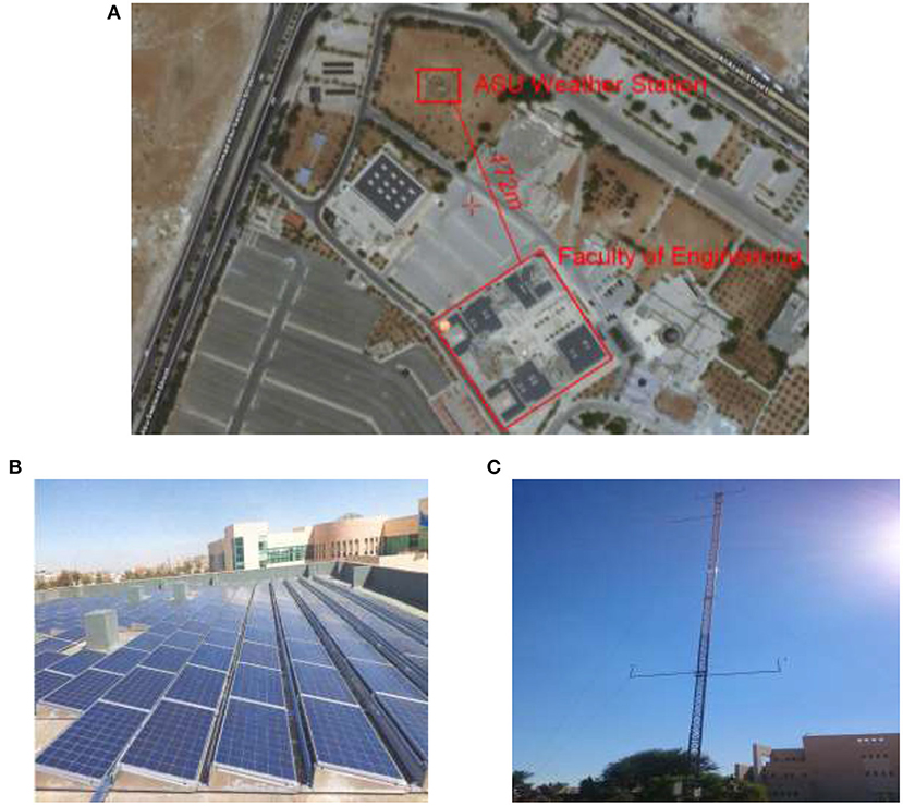
Figure 1. (A) ASU PV system map (retrieved and adapted from Google Maps, 2019). (B) ASU PV solar panels installed on the rooftop of the Faculty of Engineering. (C) ASU weather station.

The actual weather data and the associated PV power production data are collected from monitoring systems of the weather station and data loggers of the PV system, respectively. The data are collected for a period of Y = 3.75 years (from 16th May, 2015 to 31st December, 2018) with a logging interval Δt = 1 h, resulting in 31,824 rows of data [the dataset could be requested through the ASU Renewable Energy Center website at Applied Science Private University (ASU) (2019)].

ASU Solar PV System

The ASU PV system comprises 13 and 1 grid-connected solar SMA sunny tripower inverters (17 and 10 kW_ac, respectively) connected with Yingli Solar panels with peak power of 245 W, that are directly installed over concrete rooftop with 11° tilt angle and 36° azimuth angle (from South to East) [Figure 1B; Applied Science Private University (ASU), 2019].

The detailed design specifications of the ASU PV system are reported in Table 1.

TABLE 1

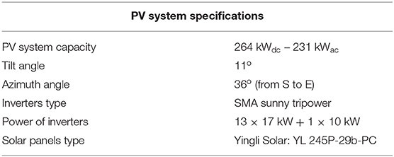
Table 1. The detailed design specifications of the ASU PV system.

ASU Weather Station

The ASU weather station (depicted in Figure 1C) is 36 m high equipped with 10 instruments for measuring the following meteorological parameters:

• Wind speed (at different levels of 10, 35, and 36 m) (m/s);

• Wind direction (at different levels of 10, 35, and 36 m);

• Ambient temperature (at different levels of 1, and 35 m) (°C);

• Relative humidity (at different levels of 1 and 35 m) (%);

• Barometric pressure (hPa);

• Precipitation amounts (mm);

• Global and diffuse solar irradiances (W/m²);

• Soil surface temperature (°C);

• Subsoil temperature (°C).

The influence of the weather features on the predictability of the PV power productions has been investigated in Alomari et al. (2018b) by developing different ANN models trained with different combinations of time and weather inputs. A combination of the current time stamp in hours, $Tim{e}_t^d$, ambient temperature at 1 m altitude, ${\vec{T}}_t^{d-e}$, and the global solar radiation, ${\vec{I}}_t^{d-e}$, measured at time t, t ∈ [1, 24], in the previous e = 5 days, was found to provide best t-th hour-ahead power production prediction of day d of the ASU solar PV system.

This work aims at exploiting, in addition to the above-mentioned features, the current time stamp as number of days, the lagged weather variables represented by the wind speed, and, in particular, the lagged actual PV power productions, to further enhance the power predictions. Thus, the input patterns of the prediction model that comprises i inputs, i = 1, …, n, at each t-th time, t ∈ [1, 24], can be written as Equation (1):

$\begin{array}{ll}{{\vec{x}}_t^d}_j=[{\overrightarrow{Time}}_t^d,{\vec{W}}_t^{d-e},{\vec{P}}_t^{d-e}],& (1)\end{array}$

where ${\vec{W}}_t^{d-e}=\left[{\vec{S}}_t^{d-e},{\vec{T}}_t^{d-e},{\vec{I}}_t^{d-e}\right]$, and the associated output of the model will be $y_{tj}^d$ = ${\widehat{P}}_{tj}^d$, for j = 1, …, N, and N is the overall number of the available inputs-outputs patterns.

It is worth mentioning that different steps are carried out a priori to process/correct the available dataset to effectively use it for the prediction task (Al-Dahidi et al., 2018; Alomari et al., 2018a; Das et al., 2018). For example, solar radiation and associated power production values are shown to be negative and missing in early and late days' hours, respectively. Such values are set to zero. Similarly, in middle days' hours, weather variables and power production values are shown to be missing as reported in Table 2 for the period Y = 3.75 years under study and, thus, are excluded from the analysis. In fact, such incorrect values are justified by either offset in the solar radiation instruments, inverter failures and/or network disruptions, or weather variables' instruments failures, respectively. Lastly, the input-output patterns are normalized to the range [0,1] to accommodate the neuron activation functions' value ranges and, consequently, enhance the ANN performance.

TABLE 2

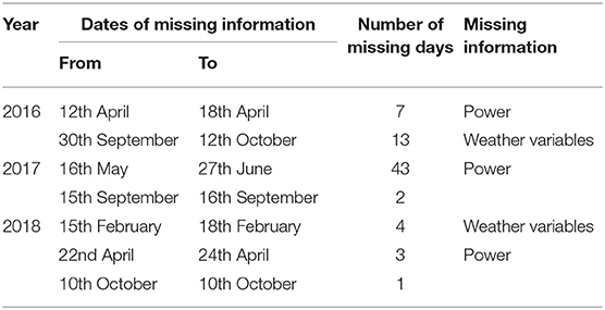
Table 2. Periods of missing weather features and power productions.

Figure 2 shows four examples of the pre-processed hourly weather variables, i.e., wind speed at 10 m altitude (Figure 2A), ambient temperature at 1 m altitude (Figure 2B), global solar radiation (Figure 2C), and the associated solar power productions (Figure 2D) in four seasons of 2016 year. One can recognize the large variability in the weather variables in the four seasons, particularly, in the wind speed at 10 m altitude, and the corresponding power productions. This is extremely important to notify for the investigation of the influence of each weather variable on the predictability of the solar power productions, as we shall see in the following sections.

FIGURE 2

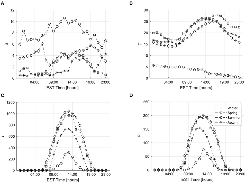
Figure 2. Few examples of the pre-processed hourly weather variables. (A) Wind speed. (B) Ambient temperature. (C) Global solar radiation. (D) The corresponding solar power production.

For completeness, Table 3 reports the yearly average weather variables [i.e., wind speed at 10 m altitude (S), ambient temperature at 1 m altitude (T), global solar radiation (I)] and the associated yearly average PV power productions (P) for the period Y = 3.75 years under study. One can notice the small variability of the reported average values of the variables that can be due to the variability in number of days of each year for which the measurements are being available (refer to Table 2) in the period under study.

TABLE 3

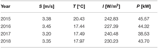
Table 3. The average yearly weather variables and the corresponding power productions of the ASU PV system for the period under study.

The whole inputs-outputs patterns are stored in the dataset matrix X and partitioned into three datasets:

• Training dataset (X_train): it holds the inputs-outputs patterns sampled randomly from the overall dataset matrix X with a fraction of 70%. This dataset, formed by N_train = 22, 192 patterns, is used to develop/train the ANN prediction model;

• Validation dataset (X_valid): it holds the inputs-outputs patterns sampled randomly from the overall dataset matrix X with the remaining fraction of 15%. This dataset, formed by N_valid = 4,756 patterns, is used to optimize the ANN model architectures in terms of number of hidden neurons and identifying the best set of features and the best ANN learning algorithm;

• Test dataset (X_test): it holds the inputs-outputs patterns sampled randomly from the overall dataset matrix X with the remaining fraction of 15%, which are never used during the ANN model development. This dataset, formed by N_test = 4, 756 patterns, is used to test/evaluate the performance of the best ANN model with respect to the Persistence (P) prediction models of literature.

Solar PV Power Prediction Modeling

The ANN model configuration proposed in this work to provide 1 day-ahead solar PV power production prediction is shown in Figure 3. ANN aims at capturing the underlying complex inputs-outputs “a priori unknown” relationship (Rumelhart et al., 1986; Hornik et al., 1989). To this aim, ANN comprises three layers through which the inputs are propagated to the outputs, they are:

• Input layer: it receives the j-th pattern, ${{\vec{x}}_t^d}_j$, that comprises one of the investigated sets of features;

• Hidden layer (composed by H hidden neurons): it processes the received inputs via a neuron activation (transfer) function, G₁(), and sends the manipulated information to the output layer;

• Output layer: it provides the t-th hour-ahead solar PV power production prediction of day d via an output neuron activation (transfer) function, G₂(), ${y_t^d}_j={\widehat{P}}_{tj}^d$, for all of the available N data patterns, j = 1, …, N, as defined by Equation (2):

$\begin{array}{ll}{{\widehat{P}}_t^d}_j=G_2\left({\displaystyle \sum _{h=1}^H{\overrightarrow{\beta }}_h{G}_1({\overrightarrow{w}}_h{{\overrightarrow{x}}_t^d}_j+b_h)}+b_o\right)& (2)\end{array}$

where ${\vec{w}}_h$, b_h, b_o, and ${\vec{\beta }}_h$ are the internal parameters of the ANN model. Specifically:

• ${\vec{w}}_h$ is the weights vector of the connections that connect the inputs features to each h-th hidden neuron (the weights' values indicate the relative importance of the inputs features to the ultimate output);

• b_h and b_o are the biases (weights) of the connections that connect the bias neurons to each h-th hidden neuron and to the output neuron, respectively. In practice, to further enhance the prediction performance of the ANN, additional neurons are added to the input (b_h) and hidden (b_o) layers which have a value of 1 (or other constant) for shifting the output of the activation functions left or right to assure that the weights' variations is sufficient to enhance the ANN prediction performance (Abuella and Chowdhury, 2015);

• ${\vec{\beta }}_h$ is the weights vector of the connections that connect the output of each h-th neuron to the output node, and

• G₁() and G₂() are the hidden and output neuron activation functions, respectively. The former is usually a continuous non-polynomial function, whereas the latter is typically a linear function (Al-Dahidi et al., 2018). The “Log-Sigmoid” has been employed as a neuron activation function following an exhaustive search procedure carried out in Al-Dahidi et al. (2018) on the same dataset of the ASU solar PV system.

FIGURE 3

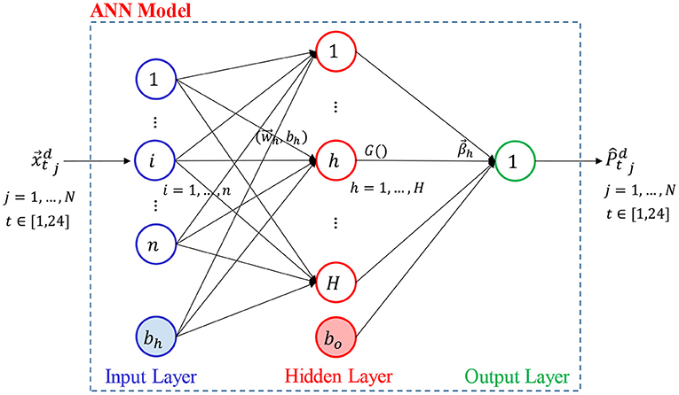
Figure 3. ANN model configuration.

In practice, the optimum ANN internal parameters, by which the outputs produced by the ANN for each input vector are sufficiently close to the desired corresponding outputs, are defined by resorting to the error Back-Propagation (BP) learning/training/optimization algorithms. During the ANN development (i.e., the training phase), the internal parameters are defined randomly, then updated iteratively while evaluating the ANN performance on the entire pair inputs-output training patterns by calculating the Mean Square Error (MSE) (i.e., the cost function) between the computed power outputs, ${\widehat{P}}_{tj}^d$ (obtained by Equation 2) and the actual power productions, $P_{tj}^d$, and distributing it back to the ANN model layers until reaching to the optimal internal parameters at which the calculated MSE is minimized.

Several learning algorithms have been widely developed and applied with success for different industrial applications. Such algorithms have different characteristics and performances in terms of computational efforts required (i.e., memory usage and computational time) and accuracy.

The idea underpinning each learning algorithm is to identify the training directions in which the ANN internal parameters are required to be updated/changed for reducing the cost/loss function. In other words, the learning algorithms differ from each other in the way in which the adjustment on the ANN internal parameters is formulated to effectively map the inputs to the outputs. It is worth mentioning that advanced meta-heuristic optimization algorithms [few to mention are Genetic Algorithm (GA) (Semero et al., 2018), Genetic Programming (GP) (De Paiva et al., 2018), Cuckoo Search (CS) (Yang and Deb, 2009), Particle Swarm Optimization (PSO) (Kennedy, 2011), Biogeography-Based Optimization (BBO) (Duong et al., 2019), Stochastic Fractal Search (SFS) and its modified version (Pham et al., 2019), or their combinations] can be employed to optimally define the ANN internal parameters. However, the influence of these algorithms on the predictability of the solar power productions could be an object of a future research work.

The influence of the learning algorithms employed to optimally define the ANN internal parameters and the sets of features considered in inputs to the ANN prediction model are described in sections ANN Learning Algorithms and ANN Training Datasets, respectively.

ANN Learning Algorithms

To propose an accurate ANN prediction model with short computational times, 10 different learning algorithms (l, l = 1, …, 10) available in MATLAB Neural Network Toolbox^TM (Demuth et al., 2009) and reported in Table 4 are investigated and their results are compared to each other for selecting the best learning algorithm.

TABLE 4

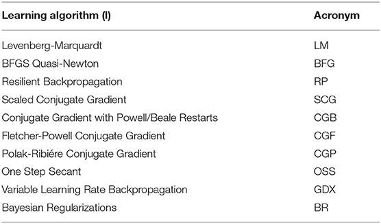
Table 4. The investigated ANN learning algorithms.

As stated previously, the learning algorithms aim to effectively map ANN inputs to outputs by optimally define the ANN internal parameters. To this aim, each algorithm adjusts the internal parameters by identifying a training direction differently from each other. Thus, each algorithm has different characteristics and performance in terms of memory usage, computational time, and accuracy. For example, Conjugate Gradient algorithms adjust the internal parameters along conjugate gradient directions, whereas the Resilient Backpropagation adjusts the internal parameters based on the sign of the slope/partial derivative of the cost function (more details on the ANN learning algorithms can be found in Demuth et al., 2009).

ANN Training Datasets

Among the available ANN inputs features [the time stamp of the year, the historical (embedding dimension) wind speed, ambient temperature, global solar radiation, and the corresponding historical PV power productions], different combinations (hereafter called sets of features) are established and investigated for an ultimate goal of providing accurate 1 day-ahead hourly power predictions. In particular, 23 sets of features, f = 1, .., 23, are established and categorized into g = 4 groups for an ease of clarity, they are (Table 5):

• Group A: it is composed by two subgroups, A′ and A^t. Specifically:

◦ A′ subgroup comprises three sets of features, each with a single weather variable, i.e., the wind speed (set A′₁), the ambient temperature (set A′₂), and the global solar radiation (set A′₃), whereas

◦ A^t subgroup combines the time span of a year and the previous three sets of features, denoted by $A_1^t$, $A_2^t$, and $A_3^t$, respectively.

TABLE 5

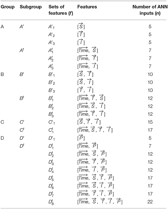
Table 5. The investigated sets of features of the ANN model.

The objectives of considering these two subgroups are to study (i) the effect of each single weather variable and (ii) the influence of the time span when combined with a single weather variable, on the predictability of the PV power production predictions;

• Group B: it is composed by two subgroups, B′ and B^t. Specifically:

◦ B′ subgroup comprises three sets of features, each with two possible combinations of the weather variable, i.e., the wind speed with the ambient temperature (set B′₁), the wind speed with the global radiation (set B′₂), and the ambient temperature with the global radiation (set B′₃), whereas

◦ B^t subgroup combines the time span of a year and the previous three sets of features, denoted by $B_1^t$, $B_2^t$, and $B_3^t$, respectively.

The objectives of considering these two subgroups are to study (i) the effect of each possible combination of two weather variables and (ii) the influence of the time span when combined with the possible pairs of the weather variables, on the predictability of the solar PV power production predictions;

• Group C: it is composed by two subgroups, C′ and C^t. Specifically:

◦ C′ subgroup comprises one set of features, composed by the three weather variables (set C′₁), whereas

◦ C^t subgroup combines the time span of a year and the previous sets of features (set $C_1^t$).

Similarly, the objectives of considering these two subgroups are to study (i) the effect of the whole three weather variables and (ii) the influence of the time span when combined with the whole weather variables, on the predictability of the solar PV power production predictions;

Finally, one of the objectives of this work is to investigate the influence of the lagged power productions on the predictability of the power production when considered as inputs to the ANN. To this aim, Group D investigates the effect of the lagged power productions by adding, incrementally, the weather variables to the lagged power productions. Therefore,

• Group D: it is composed by two subgroups, D′ and D^t. Specifically:

◦ D′ subgroup comprises one set of features, composed by the lagged power productions only (set D′₁), whereas

◦ D^t subgroup comprises eight sets of features, denoted from $D_1^t$ to $D_8^t$, by considering the lagged power productions with the time span (set $D_1^t$) incrementally reaching to the lagged power productions, the time span, and the whole considered weather variables (set $D_8^t$).

Table 5 summarizes the considered sets of features, together with their number of inputs using an embedding dimension of e = 5.

It is worth mentioning that the number of hidden neurons, H, of each ANN candidate configuration characterized by any possible combination of the above-mentioned learning algorithms (Table 4) and sets of features (Table 5), is optimized by considering different number of hidden neurons that span the interval [1,30] with a step size of 2, as we shall see in section Results and Discussions.

Performance Metrics

The performance of each ANN candidate configuration, characterized by (i) different learning algorithms (l, l = 1, …, 10), (ii) set of features (f, f = 1, .., 23), and (iii) different number of hidden neurons (H, H = [1, 30] with a step size of 2), is examined on the validation dataset, X_valid, by computing the Root Mean Square Error (RMSE), the Mean Absolute Error (MAE), and the Coefficient of Determination (R²) as standard performance metrics widely used in literature, as well as the computational time required for developing (on the validation dataset) and evaluating (on the test dataset) the built-ANN models:

• Root Mean Square Error (RMSE) [kW] (Equation 3): it describes the mismatch between the true and the predicted power productions obtained by the ANN model. Small RMSE values entail more accurate predictions and, thus, the ANN model is effectively capable of capturing the hidden mathematical relationship between the input (independent) and the output (dependent) variables, and vice versa;

$\begin{array}{ll}RMSE=\sqrt{\frac{{\displaystyle {\sum }_{j=1}^{N_{valid}}}{\left(P_j-{\widehat{P}}_j\right)}^2}{N_{valid}}}& (3)\end{array}$

• Mean Absolute Error (MAE) [kW] (Equation 4): it is defined as the average error between the true and the predicted power productions obtained by the ANN model. Similar to the RMSE performance metric, small MAE values entail more accurate predictions and, thus, the ANN model is effectively capable of capturing the hidden mathematical relationship between the input (independent) and the output (dependent) variables, and vice versa;

$\begin{array}{ll}MAE=\frac{{\displaystyle {\sum }_{j=1}^{N_{valid}}}|P_j-{\widehat{P}}_j|}{N_{valid}}& (4)\end{array}$

• Coefficient of Determination (R²) [%] (Equation 5): it is a statistical indicator that describes the variability in the output (dependent variable) power production prediction provided by the ANN models caused by the input sets of features (independent variables). In practice, R² = 100% values entail that the variability in the output variable can be fully justified by the considered input variables in the ANN prediction model, whereas R² < 100% values entail that there are other inputs (independent) variables that can influence the output variable but have not been taken into account during the development of the ANN prediction models:

$\begin{array}{ll}{R}^2=\left[1-\frac{{\displaystyle {\sum }_{j=1}^{N_{valid}}}{\left(P_j-{\widehat{P}}_j\right)}^2}{{\displaystyle {\sum }_{j=1}^{N_{valid}}}{\left(P_j-\overline{P}\right)}^2}\right]\text{ x }100\%,& (5)\end{array}$

where P_j and ${\widehat{P}}_j$ are the j-th true and predicted PV power production obtained by the ANN models, j = 1, …, N_valid and N_valid is the overall validation data patterns (i.e., N_valid = 4, 756).

• Computational time [seconds/minutes]: it is the time required for developing the ANN model candidates (on the validation dataset) and evaluating the built-ANN models (on the test dataset). Indeed, this metric is useful to identify the learning algorithm that is capable of providing as accurate as possible power production predictions, with short computational time.

Results and Discussions

To robustly evaluate the ANN prediction performance in terms of the above-mentioned metrics, a 5-fold Cross-Validation (CV) procedure is carried out. In practice, each CV trial entails sampling different training, validation, and test patterns randomly from the overall available dataset, X, with arbitrary fractions of 70, 15, and 15%, respectively. Then, the CV procedure is repeated 5 times (5-fold), by using different inputs-outputs patterns for training, validation, and test datasets. The final performance metrics values are then, computed by averaging the 5 metrics values obtained by the 5 different CV trials.

Figure 4 shows the average RMSE (Figure 4A), MAE (Figure 4B), and R² (Figure 4C) values over the 5-fold CV procedure using the 10 different learning algorithms obtained at different optimum numbers of hidden neurons. Specifically, the results of the two best learning algorithms (BR and LM in diamond and circle green markers, respectively), the three worse learning algorithms (GDX, RP, and OSS in cross, plus, upward-pointing triangle red markers, respectively), and the other remaining learning algorithms (in squares yellow marker) of each set of features are shown in the figure. Looking at Figure 4, one can recognize the following:

• The predictability of the power productions is enhanced when the time stamp (i.e., hours and number of days in a year) is fed to the ANN prediction models. This is clearly recognized when looking at the two performance metrics obtained by the models that are fed by $A_1^t$, $A_2^t$, $A_3^t$, $B_1^t$, $B_2^t$, $B_3^t$, $C_1^t$, and $D_1^t$ sets of features, compared to the metrics obtained by the models that are fed by the A₁, A₂, A₃, B₁, B₂, B₃, C₁, and D₁ sets of features, respectively. This is, indeed, justified by the fact that the PV power output depends on the sun position with respect to the PV surface (i.e., angle of incidence). In practice, the sun position depends on the location, time, and date. Thus, for a given location, including the time stamp would enhance the PV power production predictions;

• The predictability of the power productions is significantly enhanced when the solar radiation is considered together with the time stamp (i.e., set $A_3^t$) compared to $A_1^t$ and $A_2^t$. In fact, the full dependence on the solar radiation as inputs to the ANN model (i.e., A₃) rather than on the sole wind speed or ambient temperature, i.e., sets A₁ and A₂, respectively, ensures better predictability of the PV power productions. This is, indeed, expected since the PV power output, in addition to the time stamp, relies on the solar radiation. However, the influence of the other weather variables, e.g., wind speed and ambient temperature, should be, indeed, taken into account. Thus;

• The predictability of the power productions is the lowest when the sole wind speed, the ambient temperature, or the combination of these two features are fed to the ANN models, i.e., A′₁, A′₂, and B′₁, respectively. The influence of the solar radiation on the predictability of the power productions is clearly shown when the solar radiation is added to these sets of features, i.e., B′₂ and B′₃;

• The combination of the solar radiation and the time stamp as inputs to the ANN models regardless of the inclusion of the other weather variables, i.e., A′₃, B′₂, B′₃, and C′₁, slightly enhances the predictability of the power productions compared to the consideration of the solar radiation without the time stamp, i.e., $A_3^t$, $B_2^t$, $B_3^t$, and $C_1^t$, respectively;

• The inclusion of the power productions as inputs to the ANN models, i.e., Group D, is boosting the predictability of the power productions compared to the other groups, i.e., Groups A, B, and C. In fact, the best predictability is found at RMSE = 19.03 kW, MAE = 10.92 kW, R² = 91.69%, when the time stamp, the whole weather variables, and the power productions, i.e., set of features $D_8^t$, are fed to the ANN model;

• The predictability of the power productions using the BR learning algorithm (diamond green marker) is the best, i.e., RMSE = 19.03 kW, MAE = 10.92 kW, and R² = 91.69% followed by the LM algorithm (circle green marker), i.e., RMSE = 19.24 kW, MAE = 11.03 kW, and R² = 91.65%. However, the predictability using the GDX algorithm (cross red marker) is the worst among the completely investigated learning algorithms. The predictability using the other algorithms seems similar (square yellow markers). But, this performance starts to deviate toward the worse when both the RP and the OSS algorithms (plus and upward-pointing triangle red markers, respectively) being used for the latest four sets of features, i.e., $D_5^t$ to $D_8^t$.

FIGURE 4

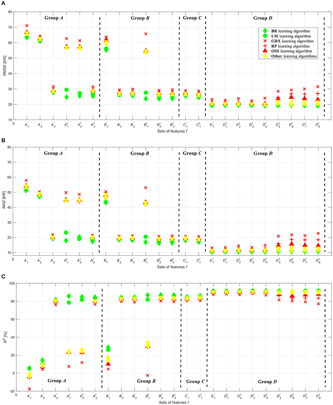
Figure 4. Average performance metrics obtained by each ANN candidate configuration on the validation dataset over 5-fold CV. (A) RMSE metric. (B) MAE metric. (C) R² metric.

For the sake of illustration, the average computational times required by each learning algorithm used for developing each ANN candidate over the 5-fold CV, considering the best set of features (i.e., $D_8^t$) and the possible numbers of hidden neurons, are shown in Figure 5. Looking at Figure 5, one can easily notice that:

• The most computational demanding is when the BR learning algorithm is used to build the ANN models and ensure convergence to optimally define their internal parameters (~30 min), whereas the other learning algorithms require almost short computational efforts (<5 min). Such huge efforts required by the BR algorithm, would, indeed, pose constraints on its practical implementation on large datasets, despite of its superior predictability results obtained in Figure 4;

• The lowest computational efforts required for developing the ANN models are obtained when the RP learning algorithm being used, i.e., <1 min. This is expected because the RP is a heuristic learning algorithm that reduces the number of learning steps and, thus, improves the convergence speed significantly, compared to the other learning algorithms (Riedmiller and Braun, 1993);

• The short computational time required by the LM algorithm, i.e., ~5 min, whose predictability is shown superior to the RP learning algorithm while slightly similar to the BR learning algorithm, increases its potentiality in real time applications.

FIGURE 5

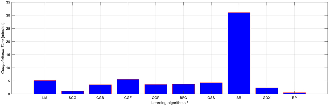
Figure 5. Average computational times required by each learning algorithm on the validation dataset.

Further insights can be obtained by looking at Figure 6 concerning the optimum number of hidden neurons, H_opt, obtained for the ANN model configuration that uses the LM learning algorithm for the $D_8^t$ set of features. Looking at Figure 6, one can generally notice the following:

• Large number of hidden neurons are required when either the wind speed and/or the ambient temperature being fed to the ANN models or when large number of inputs being fed to the ANN models. The former entails that the ANN models would try barely to correlate the wind speed and/or the ambient temperature values with those of the power production values compared, for instance, to the easily obtained correlation between the solar radiation and the power production values, whereas the latter entails that the ANN models would require more hidden neurons to capture the relationship between the inputs and the output;

• The inclusion of the time stamp in each group of sets of features facilitates the convergence, and thus, less number of hidden neurons are required;

• Even though the inclusion of most of the features (Group D) as inputs to the ANN model, the numbers of hidden neurons required tend to be similar to those required when other sets of features are considered. This indicates the fact that the inclusion of the power production as inputs to the ANN prediction model facilitates the convergence of the ANN prediction models.

FIGURE 6

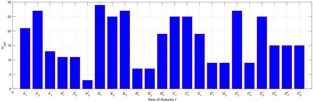
Figure 6. Optimum number of hidden neurons obtained for each set of features using the LM learning algorithm on the validation dataset.

In fact, the benefits of the utilization of the historical power productions as part of the ANN inputs set of features (e.g., $D_7^t$) compared, for instance, to the $B_3^t$ set of features (utilized in Alomari et al., 2018b using the same dataset of this work) can be easily recognize by looking at the RMSE, MAE, and R² performance metrics values. Specifically, the former leads to more accurate predictions with RMSE equals to 19.24 kW, MAE equals to 10.84 kW, and R² equals to 91.59% compared to the values of the latter with RMSE equals to 23.68 kW, MAE equals to 16.44 kW, and R² equals to 85.28%, when the BR learning algorithm being used. In addition, the BR shows the best in Alomari et al. (2018b) when looking at the predictions accuracy without any consideration of the computational efforts required for building/developing/optimizing the ANN prediction models, whereas in this work, the computational efforts are considered and showed that a compromise between the predictions accuracy and the computational efforts has to be taken into account. In practice, the convenient (short) training times of the prediction model is extremely important in real time applications such as those of the solar PV power production predictions.

In practice, one might be wondering whether the DC to AC power ratio of the ASU PV system (i.e., 1.14 in this case which is a typical practice for the PV systems design in Jordan), might influence the obtained results. This can be justified by the fact that the peak values of the global solar radiations might not always be reflected in the PV power productions because of power limitation process. However, one indication that the power limitation process has never been occurred in the ASU PV system, is that the maximum output AC power recorded in the period under study (215.33 kW_ac) is less than the system's AC rated power (i.e., 231 kW_ac).

To effectively evaluate the influence of the inclusion of the historical power productions in inputs to the ANN prediction model, the prediction performance of the ANN models built when the set of features (set $D_8^t$) is used, is compared to the performance obtained by the well-known Persistence (P) prediction model of literature, on the test dataset, X_test. Specifically, their performances are evaluated on the N_test test patterns by considering the three previously defined performance metrics, using 5-fold CV.

In P model, the solar PV power production at time t over the Δt = 24 h prediction horizon is assumed to be similar to the latest power production measured at the same time t in the previous day, as defined by Equation (6) (hereafter called Benchmark 1) (Antonanzas et al., 2016):

$\begin{array}{ll}\begin{array}{c}{\widehat{P}}_{t+\Delta t}^d=P_t^{d-1},t\in [1,24]\end{array}& (6)\end{array}$

This model is usually considered as a Baseline-prediction model and it is mostly used to compare the effectiveness of any sophisticated developed prediction model.

However, one might be wondering weather the P model can be implemented in a way that it can benefit from the historical e = 5 latest power production values (i.e., d − e, e = 1, …, 5) instead of the latest production value (i.e., d − e, e = 1), by calculateing their average value, as defined by Equation (7) (hereafter called Benchmark 2):

$\begin{array}{ll}\begin{array}{c}{\widehat{P}}_{t+\Delta t}^d=\frac{{{{\displaystyle \sum }}^{\text{}}}_{e=1}^5{P}_t^{d-e}}{5},t\in [1,24]\end{array}& (7)\end{array}$

The average performance metrics, i.e., RMSE, MAE, and R², of the power production predictions obtained resorting to the P models (Benchmark 1 and Benchmark 2) on the test dataset over the 5-CV are shown in Figure 7 in solid and dashed lines, respectively, together with those obtained by the ANN models using the best two learning algorithms (i.e., LM and BR) (bars with light shade of color) and the other learning algorithms (bars with dark shade of color). One can recognize the superiority of the developed BR and LM ANN models compared to the P benchmarks. Additionally, one can notice that the worse predictability is obtained by the developed GDX, RP, and the OS ANN models, respectively.

FIGURE 7

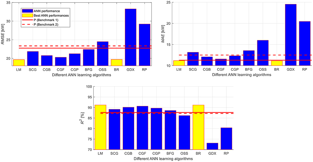
Figure 7. Average performance metrics obtained by the ANN models on the test dataset over the 5-CV using the ${\mathit{\text{D}}}_8^{\mathit{\text{t}}}$ set of features compared to the two P Benchmarks.

To effectively evaluate the effectiveness of the ANN models using the different learning algorithms with respect to the P benchmark models considering the P Benchmark 1 as a Baseline, one can compute the performance gain, PG_METRIC (%), for the RMSE and R² performance metrics as per Equation (8). In practice, positive/negative RMSE and MAE/R² performance gain values, respectively, entail the superiority of the ANN model to the Baseline-prediction model, and vice versa:

$\begin{array}{ll}P{G}_{Metric}(\%)=\frac{METRI{C}^{Baseline}-METRI{C}^{ANN}}{METRI{C}^{Baseline}}*100\%& (8)\end{array}$

Table 6 reports the performance gains obtained for the three performance metrics on the test dataset by using the ANN models equipped with the different learning algorithms with respect to the Baseline-prediction model. Looking at Table 6, one can easily recognize that the developed BR and LM ANN models largely enhance the accuracy of the PV power production predictions compared to the other investigated learning algorithms with respect to the Baseline-prediction model that obtains also a slight improvement with respect to the P2 (Benchmark 2) model.

TABLE 6

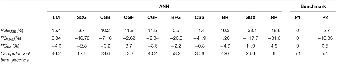
Table 6. Performance gains of the three performance metrics obtained by the ANN models using the different learning algorithms and the best set of features together with their average computational times with respect to the P models.

In addition, Table 6 reports the average computational times required by the whole prediction models. One can easily recognize that:

• The BR algorithm necessitates larger computational efforts among the whole prediction models;

• The LM algorithm necessitates shorter, and thus, convenient computational efforts compared to the BR algorithm;

• The RP algorithm necessitates shorter computational efforts among the whole ANN prediction models;

• The P prediction models, indeed, required negligible computational efforts with respect to the ANN prediction models. Despite of that, their prediction performances are not accepted.

In addition to the previous analysis, it is of paramount importance to verify whether the built-ANN on the $D_8^t$ set of features using the LM learning algorithm tends to overestimate (i.e., ${\widehat{P}}_t>P_t$) or underestimate (i.e., ${\widehat{P}}_t<P_t$) the actual t-th hourly power production of the PV system. In practice, this investigation is beneficial to propose a corrective factor for correcting the predicted power productions and further enhancing the power production predictions (Nespoli et al., 2018). In addition, the PV system owner, in particular, for a large-scale PV plants, can carry out a cost-benefit analysis to accurately quantify the benefits of the employed prediction model in terms of the overestimation and underestimation the PV power productions. To this scope, the actual PV power production values of the X_test dataset are compared to the corresponding ANN power production predictions while excluding the zero productions arise in the early morning and late evening of a day. Table 7 reports the percentages of the hourly predictions overestimating and underestimating the actual productions of the 5-fold CV trials, using N_test = 4, 756 hourly samples of the X_test dataset while excluding the zeros PV power productions. One can easily recognize the tendency of the built-ANN to slightly overestimate (i.e., ~54%) the PV power production predictions.

TABLE 7

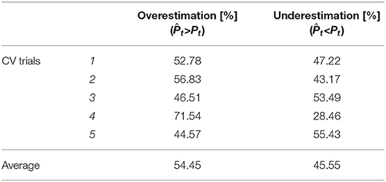
Table 7. Percentages of the hourly predictions overestimating and underestimating the actual productions on the test dataset.

For completeness, one might be wondering whether changing the embedding dimension to a lower or a higher value can influence the comparison results to the P models. To investigate the influence of the embedding dimension on the predictability of the PV power productions, different embedding dimensions that span the interval d = [1, 10] with a step size of 1 are considered, and the ANN model with LM learning algorithm, that uses the set $D_8^t$ (i.e., $\left[\overrightarrow{Time},\vec{S},\vec{T},\vec{I},\vec{P}\right]$ – 22 inputs), is built using the training dataset, X_train, optimized on the validation dataset, X_valid, for identifying the optimum number of hidden neurons, H_opt, then, evaluated on the test dataset, X_test, and compared to the P prediction models, using a 5-fold CV procedure.

In this regard, Figure 8 shows the average values of the three performance metrics on the test dataset, X_test, using the ANN model (bars) and the P prediction models (Benchmark 1 and Benchmark 2, solid and dashed lines, respectively). It can be seen that:

• The ANN model consistently outperforms the P prediction models for the different embedding dimensions, in terms of RMSE and R², which confirms the benefits of exploiting the time stamp, the historical weather variables and the PV power productions values in the development of the ANN models;

• The ANN model performs better for the intermediate embedding dimension values, i.e., d = 3 to d = 7, particularly in terms of MAE, compared to the small and large embedding dimension values. The former entails that the data used for developing the ANN models are not sufficient to capture the hidden inputs-output relationship, whereas the latter entails that considering more data for developing the ANN models leads to reduce the accuracy of the power predictions;

• The consideration of the historical power production values, d = 5, i.e., Benchmark 2 (solid line), reduces the accuracy of the predictions with respect to the consideration of the latest power production value, d = 1, i.e., Benchmark 1 (dashed line).

FIGURE 8

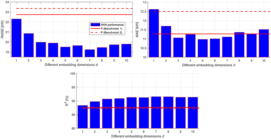
Figure 8. The influence of the embedding dimension on the prediction performance.

Conclusions

In this work, we have developed an efficient Artificial Neural Network (ANN) model for providing accurate 1 day-ahead hourly predictions of the Photovoltaics (PV) system power productions with short computational efforts. To this aim, different ANN learning algorithms for optimally defining the ANN internal parameters (i.e., weights and biases) have been investigated. In addition, different combinations of sets of features (training datasets), have been established and considered as inputs to the ANN prediction model. The sets of features are the possible combinations of the time stamp of a year, the historical actual weather variables and the corresponding PV power productions.

Specifically, several ANN models have been built using different learning algorithms and training datasets, and have been further optimized in terms of number of hidden neurons. The effectiveness of each ANN model candidate configuration has been quantified by resorting to standard performance metrics of literature, namely the Root Mean Square Error (RMSE), Mean Absolute Error (MAE), Coefficient of Determination (R²) and the computational times required to optimally define the ANN model configuration. To this aim, a 5-fold Cross-Validation (CV) procedure has been employed and the average of the 5 performance metrics values obtained by the 5 different CV trials have been reported.

The investigation is carried out on a real case study regarding a 231 kW_ac grid-connected solar PV system installed on the rooftop of Faculty of Engineering building located at the Applied Science Private University (ASU), Amman, Jordan. It has been found that the ANN model candidate configuration characterized by the combination of the time stamp of the year (in hours and number of days), the historical weather variables and PV power productions as inputs and equipped with Levenberg-Marquardt (LM) as learning algorithm, is superior to the Persistence (P) prediction model of literature, with short computational times. Specifically, an enhancement reaches up to 15, 1, and 5% for the RMSE, MAE, and R² performance metrics, respectively, with respect to the P prediction model, using 5-fold CV procedure.

The improvements obtained on the solar PV power production predictions is expected to contribute toward improving the reliability of electric power production and distribution.

Future works could be devoted toward further enhancing the prediction performance of the ANN by adopting advanced meta-heuristic optimization algorithms, e.g., Cuckoo Search (CS), for accurately optimizing the internal parameters of the ANN. Additionally, it is worth to investigate the powerful of the ensemble whose base models are the best built-ANN model of this work and whose internal parameters are optimized by resorting to CS. This is, indeed, expected to enhance the overall solar PV power production predictions. Finally, other advanced Machine Learning techniques, such as Echo State Networks (ESNs), could be promising in enhancing the predictability of the solar PV power productions by exploiting their capability of capturing the hidden stochastic nature of the weather variables and the corresponding power productions.

Data Availability Statement

The datasets generated for this study will not be made publicly available. Authors have requested the dataset utilized for this study through the ASU Renewable Energy Center website by filling in the Data Request form available at http://energy.asu.edu.jo/index.php/2016-08-29-07-34-48/forms. Moreover, Authors have signed a Non-Disclosure Agreement (NDA) for carrying their research work without circulating the data. Interested researchers can follow the same procedure.

Author Contributions

In this research activity, SA-D was involved in the conceptualization, methodology, validation, formal analysis, data analysis and pre-processing phase, software, simulation, results analysis and discussion, and manuscript preparation, review, and editing. OA, JA, and ML were involved in investigation, resources, pre-processing phase, and manuscript preparation, review, and editing. All authors have approved the submitted manuscript.

Conflict of Interest

The authors declare that the research was conducted in the absence of any commercial or financial relationships that could be construed as a potential conflict of interest.

Acknowledgments

The authors would like to acknowledge the Renewable Energy Center at the Applied Science Private University for sharing with us the Solar PV system data.

References

Abuella, M., and Chowdhury, B. (2015). Solar power forecasting using artificial neural networks, in 2015 North American Power Symposium (NAPS) (Charlotte, NC), 1–5. doi: 10.1109/NAPS.2015.7335176

CrossRef Full Text | Google Scholar

Al-Dahidi, S., Ayadi, O., Adeeb, J., Alrbai, M., and Qawasmeh, R. B. (2018). Extreme learning machines for solar photovoltaic power predictions. Energies 11:2725. doi: 10.3390/en11102725

CrossRef Full Text | Google Scholar

Al-Dahidi, S., Ayadi, O., Alrbai, M., and Adeeb, J. (2019). Ensemble approach of optimized artificial neural networks for solar photovoltaic power prediction. IEEE Access 7, 81741–81758. doi: 10.1109/ACCESS.2019.2923905

CrossRef Full Text | Google Scholar

Almonacid, F., Pérez-Higueras, P. J., Fernández, E. F., and Hontoria, L. (2014). A methodology based on dynamic artificial neural network for short-term forecasting of the power output of a PV generator. Energy Conver. Manage. 85, 389–398. doi: 10.1016/j.enconman.2014.05.090

CrossRef Full Text | Google Scholar

Alomari, M. H., Adeeb, J., and Younis, O. (2018a). Solar photovoltaic power forecasting in jordan using artificial neural networks. Int. J. Electr. Comput. Eng. 8, 497–504. doi: 10.11591/ijece.v8i1.pp497-504

CrossRef Full Text | Google Scholar

Alomari, M. H., Younis, O., and Hayajneh, S. M. A. (2018b). A predictive model for solar photovoltaic power using the levenberg-marquardt and Bayesian regularization algorithms and real-time weather data. J. Adv. Comput. Sci. Appl. 1, 347–353. doi: 10.14569/IJACSA.2018.090148

CrossRef Full Text | Google Scholar

Antonanzas, J., Osorio, N., Escobar, R., Urraca, R., Martinez-de-Pison, F. J., and Antonanzas-Torres, F. (2016). Review of photovoltaic power forecasting. Solar Energy 136, 78–111. doi: 10.1016/j.solener.2016.06.069

CrossRef Full Text | Google Scholar

Applied Science Private University (ASU) (2019). PV System ASU09: Faculty of Engineering. Available online at: http://energy.asu.edu.jo/ (accessed September 28, 2019).

Behera, M. K., Majumder, I., and Nayak, N. (2018). Solar photovoltaic power forecasting using optimized modified extreme learning machine technique. Eng. Sci. Technol. Inter. J. 21, 428–438. doi: 10.1016/j.jestch.2018.04.013

CrossRef Full Text | Google Scholar

Behera, M. K., and Nayak, N. (2019). A comparative study on short-term PV power forecasting using decomposition based optimized extreme learning machine algorithm. Eng. Sci. Technol. Int. J. doi: 10.1016/j.jestch.2019.03.006. [Epub ahead of print].

CrossRef Full Text | Google Scholar

Dahl, A., and Bonilla, E. V. (2019). Grouped gaussian processes for solar power prediction. Mach. Learn. 108, 1287–1306. doi: 10.1007/s10994-019-05808-z

CrossRef Full Text | Google Scholar

Das, U. K., Tey, K. S., Seyedmahmoudian, M., Mekhilef, S., Idris, M. Y. I., Van Deventer, W., et al. (2018). Forecasting of photovoltaic power generation and model optimization: a review. Renew. Sustain. Energy Rev. 81, 912–928. doi: 10.1016/j.rser.2017.08.017

CrossRef Full Text | Google Scholar

De Paiva, G. M., Pimentel, S. P., Leva, S., and Mussetta, M. (2018). Intelligent approach to improve genetic programming based intra-day solar forecasting models, in Proceedings of 2018 IEEE Congress on Evolutionary Computation (CEC) (Rio de Janeiro). doi: 10.1109/CEC.2018.8477845

CrossRef Full Text | Google Scholar

Demuth, H., Beale, M., and Hagan, M. (2009). Neural Network Toolbox^TM 6 User's Guide. Natick, MA: The MathWorks, Inc. Available online at: https://ch.mathworks.com/help/deeplearning/ug/choose-a-multilayer-neural-network-training-function.html;jsessionid=a36049509bedc93e8f5decfc5ff0 (accessed September 28, 2019).

Google Scholar

Duong, M. Q., Pham, T. D., Nguyen, T. T., Doan, A. T., and Van Tran, H. (2019). Determination of optimal location and sizing of solar photovoltaic distribution generation units in radial distribution systems. Energies 12:174. doi: 10.3390/en12010174

CrossRef Full Text | Google Scholar

Ernst, B., Reyer, F., and Vanzetta, J. (2009). Wind power and photovoltaic prediction tools for balancing and grid operation, in CIGRE/IEEE PES Joint Symposium Integration of Wide-Scale Renewable Resources Into the Power Delivery System (Calgary, AB), 1–9.

Google Scholar

Eseye, A. T., Zhang, J., and Zheng, D. (2017). Short-term photovoltaic solar power forecasting using a hybrid wavelet-PSO-SVM model based on SCADA and meteorological information. Renew. Energy 118, 357–367. doi: 10.1016/j.renene.2017.11.011

CrossRef Full Text | Google Scholar

Google Maps (2019). Applied Science Private University, Al Arab St, Amman. Available online at: https://goo.gl/qA4h3w (accessed September 28, 2019).

Hornik, K., Stinchcombe, M., and White, H. (1989). Multilayer feedforward networks are universal approximators. Neural Netw. 2, 359–366. doi: 10.1016/0893-6080(89)90020-8

CrossRef Full Text | Google Scholar

Kennedy, J. (2011). Particle swarm optimization, in Encyclopedia of Machine Learning, eds C. Sammut and G. I. Webb (Boston, MA: Springer), 760–766.

Google Scholar

Liu, L., Zhao, Y., Chang, D., Xie, J., Ma, Z., Wennersten, R., et al. (2018). Prediction of short-term PV power output and uncertainty analysis. Appl. Energy 228, 700–711. doi: 10.1016/j.apenergy.2018.06.112

CrossRef Full Text | Google Scholar

Malvoni, M., De Giorgi, M. G., and Congedo, P. M. (2017). Forecasting of PV power generation using weather input data-preprocessing techniques. Energy Proced. 126, 651–658. doi: 10.1016/j.egypro.2017.08.293

CrossRef Full Text | Google Scholar

Monteiro, C., Fernandez-Jimenez, L. A., Ramirez-Rosado, I. J., Muñoz-Jimenez, A., and Lara-Santillan, P. M. (2013). Short-term forecasting models for photovoltaic plants: analytical versus soft-computing techniques. Math. Prob. Eng. 2013:767284. doi: 10.1155/2013/767284

CrossRef Full Text | Google Scholar

Muhammad Ehsan, R., Simon, S. P., and Venkateswaran, P. R. (2017). Day-ahead forecasting of solar photovoltaic output power using multilayer perceptron. Neural Comput. Appl. 28, 3981–3992. doi: 10.1007/s00521-016-2310-z

CrossRef Full Text | Google Scholar

Nam, S., and Hur, J. (2018). Probabilistic forecasting model of solar power outputs based on the Naïve Bayes classifier and kriging models. Energies 11:2982. doi: 10.3390/en11112982

CrossRef Full Text | Google Scholar

Nespoli, A., Ogliari, E., Dolara, A., Grimaccia, F., Leva, S., and Mussetta, M. (2018). Validation of ANN training approaches for day-ahead photovoltaic forecasts, in Proceedings of the International Joint Conference on Neural Networks (Rio de Janeiro). doi: 10.1109/IJCNN.2018.8489451

CrossRef Full Text | Google Scholar

Nespoli, A., Ogliari, E., Leva, S., Pavan, A. M., Mellit, A., Lughi, V., et al. (2019). Day-ahead photovoltaic forecasting: a comparison of the most effective techniques. Energies 12:1621. doi: 10.3390/en12091621

CrossRef Full Text | Google Scholar

Notton, G., and Voyant, C. (2018). Chapter 3: Forecasting of Intermittent Solar Energy Resource, in Advances in Renewable Energies and Power Technologies, ed I. Yahyaoui (Elsevier), 77–114. doi: 10.1016/B978-0-12-812959-3.00003-4

CrossRef Full Text | Google Scholar

Pham, L. H., Duong, M. Q., Phan, V. D., Nguyen, T. T., and Nguyen, H. N. (2019). A high-performance stochastic fractal search algorithm for optimal generation dispatch problem. Energies 12:1796. doi: 10.3390/en12091796

CrossRef Full Text | Google Scholar

REN21 Members (2019). Renewables 2019 Global Status Report 2019. Paris: REN21 Secretariat. Available online at: https://wedocs.unep.org/bitstream/handle/20.500.11822/28496/REN2019.pdf?sequence=1&isAllowed=y (accessed September 28, 2019).

Riedmiller, M., and Braun, H. (1993). A direct adaptive method for faster backpropagation learning: the RPROP algorithm, in Proceedings of IEEE International Conference on Neural Networks (San Francisco, CA). doi: 10.1109/ICNN.1993.298623

CrossRef Full Text | Google Scholar

Rumelhart, D. E., Hinton, G. E., and Williams, R. J. (1986). Learning representations by back-propagating errors. Nature 323, 533–536. doi: 10.1038/323533a0

CrossRef Full Text | Google Scholar

Semero, Y. K., Zhang, J., and Zheng, D. (2018). PV power forecasting using an integrated GA-PSO-ANFIS approach and gaussian process regression based feature selection strategy. CSEE J. Power Energy Syst. 4, 210–218. doi: 10.17775/CSEEJPES.2016.01920

CrossRef Full Text | Google Scholar

VanDeventer, W., Jamei, E., Thirunavukkarasu, G. S., Soon, T. K., Horan, B., Mekhilef, S., et al. (2019). Short-term PV power forecasting using hybrid GASVM technique. Renew. Energy 140, 367–379. doi: 10.1016/j.renene.2019.02.087

CrossRef Full Text | Google Scholar

Wan, C., Zhao, J., Member, S., and Song, Y. (2015). Photovoltaic and solar power forecasting for smart grid energy management. J. Power Energy Syst. 1, 38–46. doi: 10.17775/CSEEJPES.2015.00046

CrossRef Full Text | Google Scholar

Wang, J., Zhong, H., Lai, X., Xia, Q., Wang, Y., and Kang, C. (2019). Exploring key weather factors from analytical modeling toward improved solar power forecasting. IEEE Trans. Smart Grid 10, 1417–1427. doi: 10.1109/TSG.2017.2766022

CrossRef Full Text | Google Scholar

Wolff, B., Kühnert, J., Lorenz, E., Kramer, O., and Heinemann, D. (2016). Comparing support vector regression for PV power forecasting to a physical modeling approach using measurement, numerical weather prediction, and cloud motion data. Solar Energy 135, 197–208. doi: 10.1016/j.solener.2016.05.051

CrossRef Full Text | Google Scholar

Yagli, G. M., Yang, D., and Srinivasan, D. (2019). Automatic hourly solar forecasting using machine learning models. Renew. Sustain. Energy Rev. 105, 487–498. doi: 10.1016/j.rser.2019.02.006

CrossRef Full Text | Google Scholar

Yang, H. T., Huang, C. M., Huang, Y. C., and Pai, Y. S. (2014). A weather-based hybrid method for 1-day ahead hourly forecasting of PV power output. IEEE Trans. Sustain. Energy 5, 917–926. doi: 10.1109/TSTE.2014.2313600

CrossRef Full Text | Google Scholar

Yang, X.-S., and Deb, S. (2009). Cuckoo search via levy flights, in 2009 World Congress on Nature & Biologically Inspired Computing (NaBIC) (Coimbatore). doi: 10.1109/NABIC.2009.5393690

CrossRef Full Text

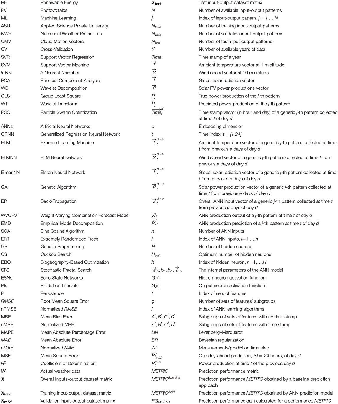
Notations