Three-Phase Four-Wire OPF-Based Collaborative Control of PV Inverter and ESS for Low-Voltage Distribution Networks With High Proportion PVs

Introduction

In recent years, with the rapid development of economy, environmental pollution and the energy crisis are being increasingly prominent. In order to achieve the sustainable energy development, photovoltaic and other renewable energy power generation has been vigorously promoted (Zehar and Sayah, 2008). However, large-scale household photovoltaic integration will affect the node voltage and network losses of the three-phase four-wire structure of the low-voltage distribution network. The mismatch between household photovoltaic generation and household loads causes the violation of the upper voltage limit during the day and the lower limit in the evening (Aziz and Ketjoy, 2017). In addition, the three-phase four-wire structure of the low-voltage distribution network will lead to three-phase unbalances if there are three-phase loads and asymmetric line parameters (Pansakul and Hongesombut, 2014). Therefore, it is significant to research on the photovoltaic utilization for a three-phase four-wire system of the low-voltage distribution network.

At present, a large amount of literature has been carried out on photovoltaic utilization in the distribution network. Voltage control can be performed by adjusting the on-load tap-changer tap position (Liu et al., 2012). However, as a result of the limitation in the tap position, the amount of voltage regulation is non-continuous. Also, frequently regulation of taps will cause the reduction in transformers service life. Another method is to reduce the photovoltaic active power (Tonkoski, 2009; Reinaldo et al., 2011) to suppress the occurrence of over-voltage, however, this will reduce the income of photovoltaic owners. In addition, this method only performs voltage control and will not improve the photovoltaic utilization of the distribution network. The photovoltaic inverter’s reactive power regulation capability (Qian et al., 2018) can be used to achieve photovoltaic utilization. Compared with the previous two methods, this method has a smoother controllable volume, and will not require additional investment or loss of generation revenues. However, there may be shortcomings of insufficient reactive power resulting in unsatisfactory voltage control. At present, energy storage equipment is also widely used in the voltage control after the low-voltage distribution network is connected to photovoltaic. In particular, a large number of literatures have studied the coordinated control method of energy storage and reactive power inverter (Zhang et al., 2020). This strategy can effectively suppress the voltage over limit, make full use of equipment capacity through the coordination of equipment, greatly reduce the cost of voltage regulation and network loss. Although there is one more neutral line in the three phase four wire system than the three phase four wire system, the control strategy adopted by the three phase three wire system is still applicable to the three phase four wire system. Therefore, if the investment cost is considered, for the three-phase three-wire low-voltage distribution network and the three-phase four-wire low-voltage distribution network with the same load and control equipment, there is only a neutral line gap in their investment costs.

The OPF problem of the distribution network needs to consider the feasibility of the model and the solution. In terms of the model, the OPF problem is to find the optimal state of a controllable variable of the power grid, so that the objective functions such as network loss and operating cost of the distribution network will reach the optimization. Literature (Gill et al., 2014) is based on the premise of ensuring the safe operation of the power grid, and aims at maximizing the photovoltaic power generation and its benefits to establish a dynamic optimal power flow model of an active power distribution network. Literature (Alsenani and Paudyal, 2018) aims to minimize the network loss by proposing an OPF model to solve the three-phase unbalance in the distribution network. However, the above literature ignores that the low-voltage distribution network is actually a three-phase four-wire system. The neutral wire makes the three-phase three-wire system and the three-phase four-wire system essentially different in calculation methods and other aspects (Bozchalui and Sharma, 2014). The neutral line voltage and current, and the phase line voltage and current should meet the Kirchhoff's law, which cannot be directly obtained through methods similar with the symmetrical components in a three-phase three-wire system. The three-phase three-wire model cannot accurately reflect the three-phase unbalance. However, there are relatively few researches on the OPF model of three-phase four-wire system.

For the OPF solution, scholars have established the OPF model as a linear or non-linear programming model and directly solved it based on artificial intelligence algorithms such as genetic algorithm (Martins and Carmenlt, 2011), particle swarm algorithm (Niknam et al., 2012), etc. However, the solution speed is slow and can easily fall into local optimization instead of the global. Other scholars used the convex model of convexity relaxation, which first eliminated the phase angle of voltage and current, and then used a second-order cone relaxation to convexify the original model (Bose et al., 2016; Tian et al., 2016; Ju et al., 2017; Zafar et al., 2020). However, since OPF solutions such as second-order cones need to eliminate the phase angle between voltage and current, this method cannot calculate the voltage and current on the neutral line. Therefore, it cannot be applied to three-phase four-wire system. The research at present is only to solve some specific problems, such as the minimization of network loss, three-phase unbalance, etc. Few Hardly any attention has been paid to the actual three-phase four-wire system model of low-voltage distribution networks. No effective solution method has been proposed for the three-phase four-wire OPF model. It is hence necessary to propose a calculation method for OPF of a three-phase four-wire distribution network.

The main contributions of this paper are summarized as follows.

(1) Due to the lack of research on three-phase four-wire SYSTEM OPF model in existing literature studies, this paper establishes an OPF model based on the optimal coordinated control of photovoltaic power generation and energy storage for three-phase four-wire low-voltage distribution network, aiming at network loss, three-phase imbalance and voltage deviation, and taking neutral line voltage, photovoltaic and energy storage as constraints.

(2) As it is discussed that the OPF solution method in present research is not applicable to the model in this paper, a convex process solution of optimal power flow model based on photovoltaic utilization in the low-voltage distribution network is proposed. Based on the established three-phase four-wire low-voltage distribution network optimal power flow model, all the concave functions in the model are converted into convex functions, Thereafter, the three-phase four-wire OPF model can be efficiently solved.

The remaining paper is structured as follows. Section 2 provides the mathematical formulations of the three-phase four-wire low-voltage distribution network topology and low-voltage components containing photovoltaic and energy storage. Section 3 establishes the coordinated control model of photovoltaic and energy storage in a three-phase four-wire system low-voltage distribution network. Section 4 proposes a solution method based on the three-phase four-wire optimal power flow. Section 5 obtains the effectiveness of the proposed optimization method through simulation. Section 6 concludes the study.

Three-phase Four-Wire Low Voltage Distribution Network Equation With Photovoltaic and Energy Storage Headings

Network Equations Containing Photovoltaic and Energy Storage in a Three-phase Four-Wire Low Voltage Distribution Network

Network Topology of a Three-phase Four-Wire Low Voltage Distribution Network

The low-voltage distribution network (LVDN) in China adopts a three-phase four-wire structure. The distribution network model between two busbars (m-1) and m is shown in Figure 1. This model has only one reference node, which is the neutral node at the beginning of the line. All other nodes take this as the reference point. The model contains two busbars (m-1) and m. Each busbar consists of four nodes, which are (4i-3), (4i-2), (4i-1), (4i), and (4j-3), (4j-2), (4j-1), and (4j) representing the three phases of a, b, and c on busbars (m-1) and m respectively, and the neutral line n. Each phase line has its own impedance, and the coupling relationship between each phase line is expressed by mutual impedance. Phase a, b, and c lines are connected to the neutral line through a load to form a closed loop.

FIGURE 1

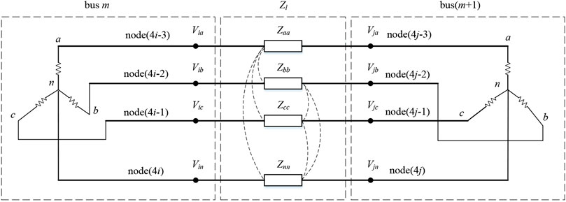
FIGURE 1. Model of the three-phase four-wire low voltage distribution network.

Branch Model

According to the topology of the LVDN, the three-phase four-wire system between any two busbars (m-1) and m can be represented by a 4 × 4 series impedance matrix.

$Z_{l,m}=\left[\begin{array}{cccc}{Z}_{aa}& Z_{ab}& Z_{ac}& Z_{an}\\ Z_{ba}& Z_{bb}& Z_{bc}& Z_{bn}\\ Z_{ca}& Z_{cb}& Z_{cc}& Z_{cn}\\ Z_{na}& Z_{nb}& Z_{nc}& Z_{nn}\end{array}\right](1)$

where Z_gg is the diagonal element of the series impedance matrix, which is the self-impedance of the three phases of a, b, and c and the neutral line n; Z_gh is the off-diagonal element of series impedance matrix $\left(g\ne h\right)$ which is the mutual impedance between three-phase a, b, c and neutral line n.

In order to obtain the overall model of the LVDN, the calculation formulas are all in matrix. Therefore, the admittance matrix Y of a LVDN node with m buses can be expressed as:

$Y_l=\left[\begin{array}{ccc}{Z}_{l,1}^{-1}+{\displaystyle \sum _{k\in c\left(1\right)}{Z}_{l,k}^{-1}}& \cdots & -\left(Z_{l,m}^{-1}+{\displaystyle \sum _{k\in c\left(m\right)}{Z}_{l,k}^{-1}}\right)\\ ⋮& \ddots & ⋮\\ -\left(Z_{l,m}^{-1}+{\displaystyle \sum _{k\in c\left(m\right)}{Z}_{l,k}^{-1}}\right)& \cdots & Z_{l,m}^{-1}+{\displaystyle \sum _{k\in c\left(m\right)}{Z}_{l,k}^{-1}}\end{array}\right](2)$

where c (m) represents the set of busbars connected with the busbar m; $Z_{l,m}^{-1}$ is the inverse matrix of the series impedance matrix connected between the busbars (m-1) and m; ${\displaystyle \sum _{k\in c\left(m\right)}{Z}_{l,k}^{-1}}$ is the sum of the inverse matrices of all the series impedance matrix connected to busbar m.

Substituting Eq 1 into Eq 2, the overall node admittance matrix of the LVDN can be obtained.

$Y=\left[\begin{array}{cccccc}{Y}_{l11}& Y_{l12}& \cdots & Y_{l12}& \cdots & Y_{l1N}\\ Y_{l21}& Y_{l22}& \cdots & Y_{l2i}& \cdots & Y_{l2N}\\ ⋮& ⋮& \ddots & ⋮& \ddots & ⋮\\ Y_{li1}& Y_{li2}& \cdots & Y_{lii}& \cdots & Y_{liN}\\ ⋮& ⋮& \ddots & ⋮& \ddots & ⋮\\ Y_{lN1}& Y_{lN2}& \cdots & Y_{lNN}& \cdots & Y_{lNN}\end{array}\right](3)$

where N represents the number of nodes in the LVDN.

Load Connections in an Low-Voltage Distribution Network

Photovoltaic energy storage into low-voltage distribution network technology is very common, effective use of clean energy and distribution network voltage control has a very obvious effect.

As shown in Figure 2, taking phase b as an example. The photovoltaic, load and energy storage are connected to a single-phase in the distribution network. Phase b and the neutral line n are connected to form a closed loop.

FIGURE 2

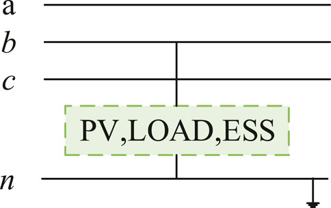
FIGURE 2. Illustration of PV, LOAD and ESS connection at phase b.

Photovoltaic, load and energy storage all use a constant power model to obtain the injection current at node i.

$I_i\left(t\right)=\frac{\left(P_{PV,i}\left(t\right)+P_{ESS,i}\left(t\right)-P_{LOAD,i}\left(t\right)\right)-j\left(Q_{PV,i}\left(t\right)-Q_{LOAD,i}\left(t\right)\right)}{U_{\phi ,i}^{\ast }}(4)$

where $P_{PV,i}\left(t\right)$, $Q_{PV,i}\left(t\right)$ represent the photovoltaic active power and reactive power of node i at time t; $P_{LOAD,i}\left(t\right)$, $Q_{LOAD,i}\left(t\right)$ represent the active and reactive power of load at node i at time t; $P_{ESS,i}\left(t\right)$ represents the active power of energy storage at node i at time t. If no energy storage is connected, the value is 0.

Storage Model

Regulating the energy storage charge and discharge power is an effective way to control the voltage. When the photovoltaic power generation is large during the day and cannot be completely absorbed by the power grid, excessive energy can be absorbed through energy storage. Energy storage releases active power to compensate for the power shortage of the grid in the evening when photovoltaic is not generating and the power demand is high. The State of Charge (SOC) of energy storage is an important indicator for measuring the capacity of charge and discharge of energy storage. It represents the ratio of the remaining charge and discharge capacity of the energy storage system to its fully storage capacity. It is expressed as a percentage. The value range is [0,1]. The SOC at the next time step is closely related to the SOC at the present time step. The energy storage SOC can be expressed as:

$SO{C}_{ESS,i}\left(t+\Delta t\right)=SO{C}_{ESS,i}\left(t\right)-\frac{P_{ch\mathrm{arge},i}\left(t\right){\eta }_{ch\mathrm{arge}}\Delta t}{E_N}+\frac{P_{disch\mathrm{arge},i}\left(t\right)\Delta t}{{\eta }_{disch\mathrm{arge}}{E}_N}(5)$

where $SO{C}_{ESS,i}\left(t\right)$ represents the energy storage SOC of node i at time t; $SO{C}_{ESS,i}\left(t+\Delta t\right)$ represents the energy storage SOC of node i at the next time step; Δt is the time interval; E_N is the energy storage capacity; ${\eta }_{ch\mathrm{arge}}$, ${\eta }_{disch\mathrm{arge}}$ are the charging efficiency and discharge efficiency of the energy storage; At time t, $P_{ch\mathrm{arge},i}\left(t\right)$, $P_{disch\mathrm{arge},i}\left(t\right)$ represents the storage charging power and discharging power of node i.

Photovoltaic Inverter Model

The model makes full use of the reactive power of photovoltaic inverters for voltage regulation. The photovoltaic absorbs reactive power to reduce the overvoltage and generates reactive power to raise the undervoltage. The relationship between the adjustable reactive power capacity and inverter is

$Q_{PV,\phi }^{\max }=\pm \sqrt{S_{PV,\phi }^2-P_{PV,\phi }^2},\phi \in abc(6)$

where $Q_{PV,\phi }^{\max }$ is the maximum output of reactive power of the inverter that is installed in the phase φ (node i). S_pv,φ is the rated capacity of the PV inverter installed in phase φ, which is 1.1 times of the rated active power. P_pv,φ is the Photovoltaic active power installed in the phase φ.

Matrix of Three-phase Four-Wire Power Flow Algorithm for Low-Voltage Distribution Network

According to the circuit theory, the node voltage and current should satisfy the node voltage equation. In the three-phase four-wire system, the node voltage equation of the LVDN can be obtained through the node admittance matrix.

$\left[Y\right]\cdot \left[V\left(t\right)\right]=\left[I_{in}\left(t\right)\right](7)$

where $\left[V\left(t\right)\right]$ represents a matrix containing the voltage of each node at time t, its dimension is N × 1; $\left[I_{in}\left(t\right)\right]$ is a matrix composed of the current injected by each node at time t, and its dimension is N × 1. Each element $I_i\left(t\right)$ of the matrix $\left[I_{in}\left(t\right)\right]$ can be obtained by Eq 4.

In order to obtain the voltage of each node, Eq 7 can be modified

$\left[V\left(t\right)\right]={\left[Y\right]}^{-1}\left[I_{in}\left(t\right)\right](8)$

By solving Eq 8, the voltage of each node can be obtained.

$\left[\begin{array}{c}{V}_1\left(t\right)\\ V_2\left(t\right)\\ ⋮\\ V_i\left(t\right)\\ ⋮\\ V_N\left(t\right)\end{array}\right]={\left[\begin{array}{cccccc}{Y}_{l11}& Y_{l12}& \cdots & Y_{l1i}& \cdots & Y_{l1N}\\ Y_{l21}& Y_{l22}& \cdots & Y_{l2i}& \cdots & Y_{l2N}\\ ⋮& ⋮& \ddots & ⋮& \ddots & ⋮\\ Y_{li1}& Y_{li2}& \cdots & Y_{lii}& \cdots & Y_{liN}\\ ⋮& ⋮& \ddots & ⋮& \ddots & ⋮\\ Y_{lN1}& Y_{lN2}& \cdots & Y_{lNi}& \cdots & Y_{lNN}\end{array}\right]}^{-1}\left[\begin{array}{c}{I}_1\left(t\right)\\ I_2\left(t\right)\\ ⋮\\ I_i\left(t\right)\\ ⋮\\ I_N\left(t\right)\end{array}\right](9)$

However, the node admittance matrix $\left[Y\right]$ is singular matrix, which can not be inverse. Therefore, it is necessary to improve the node admittance matrix $\left[Y\right]$.

$Y^{\text{'}}=\left[\begin{array}{cccccc}E& 0& \cdots & 0& \cdots & 0\\ Y_{l51}& Y_{l52}& \cdots & Y_{l5i}& \cdots & Y_{l5N}\\ ⋮& ⋮& \ddots & ⋮& \ddots & ⋮\\ Y_{li1}& Y_{li2}& \cdots & Y_{lii}& \cdots & Y_{liN}\\ ⋮& ⋮& \ddots & ⋮& \ddots & ⋮\\ Y_{lN1}& Y_{lN2}& \cdots & Y_{lNi}& \cdots & Y_{lNN}\end{array}\right](10)$

where E is identity matrix with a dimension of 4 × 4.

The Coordinated Control Model of Photovoltaic and Energy Storage in Three-phase Four-Wire Low-Voltage Distribution Network

The coordinated control method of photovoltaic and energy storage for the three-phase four-wire low-voltage distribution network proposed in this paper refers to the control idea proposed in (Zhang et al., 2020), which is a two-stage distributed control strategy for inverter and energy storage. It adjusts the reactive power of the inverter first and then adjusts the active power of the energy storage during voltage control.

Objective Function

The optimization control of the LVDN involves multiple optimization objectives. In this paper, minimize the network loss, the three-phase unbalance and the voltage deviation are the objectives. The three-phase four-wire system OPF model is established. The optimization variables are photovoltaic reactive power and energy storage active power. The multi-objectives problem is converted to a single-objective problem by weighting. The overall objective function can be expressed as

$\min F={{\omega }_{1}F/F_{1ref}}_1+{\omega }_2{F}_2/F_{2ref}+{\omega }_3{F}_3/F_{3ref}(11)$

where F is the objective function value; F₁, F₂, F₃ are the objective function value of network loss, three-phase unbalance and voltage deviation; F_1ref, F_2ref, and F_3ref are the reference values of each objective function, which is used as a reference to standardize each objective function to per unit. In this paper, the network loss, three-phase unbalance and voltage deviation without control are used as the reference values. ω₁, ω₂ and ω₃ are the weight values of each objective function, and should meet ${\omega }_1+{\omega }_2+{\omega }_3=1$, and ${\omega }_1\ge \text{0}$, ${\omega }_2\ge \text{0}$, ${\omega }_3\ge \text{0}$.

(1) Network losses

Network loss is an important indicator for measuring the economy of the LVDN. The objective function for calculating the network losses of the LVDN is:

$F_1={\displaystyle \sum _{t=1}^T{P}_{loss}\left(t\right)\cdot \Delta t}={\displaystyle \sum _{t=1}^T{\left[{\left[I_{line}\left(t\right)\right]}^{\ast }\otimes \left[I_{line}\left(t\right)\right]\right]}^T\cdot \left[R\right]\cdot \Delta t}(12)$

where $\left[I_{line}\left(t\right)\right]={\left[I_{line,1}^{abc}\left(t\right)I_{line,1}^n\left(t\right)\cdots I_{line,\left(m-1\right)}^{abc}\left(t\right)I_{line,\left(m-1\right)}^{abc}\left(t\right)\right]}^T$; $\left[R\right]={\left[R_1^{abc}{R}_1^n\cdots R_{\left(m-1\right)}^{abc}{R}_{\left(m-1\right)}^n\right]}^T$; $\left[I_{line}\left(t\right)\right]$ represents a complex matrix containing the amplitude and phase angle of the branch current at time t, with a dimension of l×1, where l represents the number of branches in the distribution network; $\left[I_{line,m}^{abc}\left(t\right)\right]$ represents the three phases currents of a, b and c on the m-segment line at time t, with a dimension of 3 × 1; $\left[I_{line,m}^n\left(t\right)\right]$ represents the current of the neutral line n on the m-segment line at time t, with a dimension of l × 1; R is the branch resistance with a dimension of l × 1; $R_m^{abc}$ includes the resistance value of three phases of a, b and c on the m-segment line, with a dimension of 3 × 1; $R_m^n$ represents the resistance value of neutral line n on the m-segment line, with dimension of l × 1. A new operation symbol $\otimes$ is defined, which represents the multiplication of the corresponding elements of two matrices.

(2) Three-phase unbalance factor

Voltage Unbalance Factor (VUF) is also an important indicator in LVDN. The definition can be the ratio of the negative sequence fundamental component to the positive sequence fundamental component.

$U_{\text{VUF},m}\left(t\right)=\left|\frac{V_{-,m}\left(t\right)}{V_{+,m}\left(t\right)}\right|=\left|\frac{V_{\mathrm{a},m}\left(t\right)+\alpha V_{\mathrm{b},m}\left(t\right)+{\alpha }^2{V}_{\mathrm{c},sm}\left(t\right)}{V_{\mathrm{a},m}\left(t\right)+{\alpha }^2{V}_{\mathrm{b},m}\left(t\right)+\alpha V_{\mathrm{c},m}\left(t\right)}\right|(13)$

where $V_{\mathrm{a},m}\left(t\right)$, $V_{\mathrm{b},m}\left(t\right)$, $V_{\mathrm{c},m}\left(t\right)$ represent the voltage of each phase at bus m; $V_{-,m}\left(t\right)$ represents the negative sequence voltage; $V_{+,m}\left(t\right)$ represents the positive sequence voltage; $\alpha =1\angle {120}^{\circ }$.

Take the minimization of the three-phase unbalance of each bus in the distribution network as the objective function:

$F_2={\displaystyle \sum _{t=1}^T{\displaystyle \sum _{i=1}^l{U}_{\text{VUF},m}\left(t\right)}}(14)$

where l represents the number of branches in LVDN.

(3) Voltage deviation

The difference between the actual voltage of each point and the nominal voltage of the system is called the voltage deviation. The objective function for calculating the voltage deviation of the LVDN is:

$\Delta U_{\phi }={\left(\frac{U_{\phi ,m}\left(t\right)-U_N}{U_N}\right)}^2(15)$

$F_{3=}{\displaystyle \sum _{t=1}^T{\displaystyle \sum _m{\displaystyle \sum _{\phi \in abc}\Delta U_{\phi }}}}(16)$

where $\Delta U_{\phi }$ represents the voltage deviation of a certain phase at a certain node at a certain time; U_N represents the standard voltage of the system.

The selection of the target weight mainly considers the importance of different indicators in the optimization model. As the network losses is closely related to the operating cost of the distribution network, the smaller the value, the better the results. The three-phase unbalance is according to the requirements of GB/T 12,325–2008 “Power Quality Three-Phase Voltage Unbalance”. The allowable value of the voltage unbalance at the public connection point of the power system during normal operation of the power grid is 2%, and it must not exceed 4% in a short time. That is, the VUF that is less than 2% can meet the requirements. Therefore, economics (network losses) is the primary concern of the optimization model in this paper, and its weight should be greater than the three-phase unbalance weight. This paper first takes the weights of the two objective functions as 0.85 and 0.15. The effect of different weights on the control effect will be analyzed in more detail in the case study section.

Constraints

(1) Branch current constraints

$\left|I_{ij}\left(t\right)\right|\le I_{ij,max}(17)$

where $I_{ij}\left(t\right)$ represents the current of branch ij that connects node i and node j; $I_{ij,max}$ represents the maximum allowable value of the branch current. This paper uses 100A.

(2) Voltage constraints

For the voltage amplitude of each node on a, b, and c phase, according to national standards, there should be a maximum and minimum limit to ensure the safe operation of the power grid.

$V_{i,min}\le \left|V_i\left(t\right)\right|\le V_{i,max}(18)$

where $\left|V_i\left(t\right)\right|$ represents the voltage amplitude of node i at time t; $V_{i,min}$ represents the minimum allowable voltage at node i, $V_{i,max}$ represents the maximum allowable voltage. According to GB/T 12,325–2008 “Power Quality Voltage Allowable Range”, the 220V single-phase supply voltage deviation is −10%–7% of the nominal voltage.

(3) Neutral line voltage constraints

$\left|V_{i,neutral}\left(t\right)\right|\le V_{neutral,max},i\in n(19)$

where $\left|v_{i,neutral}\left(t\right)\right|$ represents the voltage amplitude of node i on the neutral line at time t; $V_{neutral,max}$ represents the maximum allowable value of the neutral line voltage. According to DL/T 620–1997 “Overvoltage Protection and Insulation Coordination for AC Electrical Installations”, the neutral point voltage displacement rate should be less than 15% of the phase voltage.

(4) Photovoltaic inverter capacity constraints

The reactive power of photovoltaic inverters is not unlimited, and the active power and capacity of photovoltaic inverters must meet certain constraints.

$P_{\phi }^2+Q_{\phi }^2\le S_{\phi }^2,\phi \in abc(20)$

where P_φ indicates the active power of the photovoltaic inverter connected to the phase ^φ; Q_φ indicates the reactive power of the photovoltaic inverter connected to the phase ^φ; S_φindicates the capacity of the photovoltaic inverter connected to the phase ^φ.

(5) Energy storage constraints

The limits of SOC at time t:

$SO{C}_{ESS,min}\le SO{C}_{ESS,i}\left(t\right)\le SO{C}_{ESS,max}(21)$

where $SO{C}_{ESS,min}$, $SO{C}_{ESS,max}$ represent the minimum and maximum allowable SOC of energy storage. This paper takes 20 and 80%.

Take a day as a charge and discharge cycle of the energy storage device, the initial state of each cycle should be the same.

$SO{C}_{ESS,i}\left(t_0\right)=SO{C}_{ESS,i}\left(t_n\right)(22)$

where $SO{C}_{ESS,i}\left(t_0\right)$ represents the initial SOC of a day, $SO{C}_{ESS,i}\left(t_n\right)$ represents the SOC at the end of a day.

In addition, energy storage should meet the charging and discharging power constraints.

$\{\begin{array}{l}{P}_{charge,i,min}{D}_{charge,i}\left(t\right)\le P_{charge,i}\left(t\right)\le P_{charge,i,max}{D}_{charge,i}\left(t\right)\\ P_{discharge,i,min}{D}_{discharge,i}\left(t\right)\le P_{discharge,i}\left(t\right)\le P_{discharge,i,max}{D}_{discharge,i}\left(t\right)\\ D_{charge,i}\left(t\right)+D_{discharge,i}\left(t\right)\le 1\end{array}(23)$

where $P_{charge,i,min}$ , $P_{charge,i,max}$ represent the minimum and maximum values of energy storage charging power; $P_{discharge,i,min}$, $P_{discharge,i,max}$ represent the minimum and maximum values of energy storage discharge power; $D_{charge,i}\left(t\right)$, $D_{discharge,i}\left(t\right)$ are binary variables.

(6) Tie line power constraints

After a high proportion of photovoltaics are integrated, there will be a phenomenon of power flow from the LVDN to the upper-level power grid. In order to ensure the normal operation of each device, the tie line between the low voltage station area and the upper-level power grid should meet the power limit.

$P_{con,min}\le P_{con}\left(t\right)\le P_{con,max}(24)$

where $P_{con,min}$, $P_{con,max}$ represent the upper and lower limit of the tie line. The value should not be greater than the rating of the distribution transformer. $P_{con}\left(t\right)$ represents the actual power of the tie line at time t.

Solution Method Based on Optimal Power Flow Model in a Three-phase Four-Wire System

This paper uses the complex form to represent both the magnitude and phase angle of the variables, and the optimization model contains non-convex nonlinear constraints. Therefore, the OPF problem is a non-convex programming problem. It is difficult to obtain a global optimal solution. In order to solve the problem, all variables are split into real part and imaginary part. For Eq 8, it can be simplified by the following formula.

$\left[V\right]=\left[V_{re}+j{V}_{re}\right]={\left[\mathrm{Re}\left(Y\right)+\mathrm{Im}\left(Y\right)\right]}^{-1}\cdot \left[I_{in,re}+j{I}_{in,im}\right](25)$

Therefore, the real and imaginary part of each node voltage can be represented:

$\left[V_{re}\right]={\left[\mathrm{Re}\left(Y\right)\right]}^{-1}\cdot \left[I_{in,re}\right]-{\left[\mathrm{Im}\left(Y\right)\right]}^{-1}\cdot \left[I_{in,im}\right](26)$

$\left[V_{im}\right]={\left[\mathrm{Im}\left(Y\right)\right]}^{-1}\cdot \left[I_{in,re}\right]+{\left[\mathrm{Re}\left(Y\right)\right]}^{-1}\cdot \left[I_{in,im}\right](27)$

(1) Upper voltage constraint

The voltage is split into real and imaginary parts. The essence of the upper voltage constraint is that the modulus length of the complex number is less than the specified value.

$V_{i,re}^2\left(t\right)+V_{i,im}^2\left(t\right)\le V_{i,max}^2(28)$

where $V_{i,re}\left(t\right)$ represents the real part of node i voltage at time t; $V_{i,re}\left(t\right)$ represents the imaginary part of node i voltage at time t; $V_{i,max}$ represents the maximum allowable value of node i voltage.

(2) Lower voltage constraint

The voltage lower voltage constraint is a concave function, which is difficult to solve and hard to maintain the optimality of the solution. Therefore, this constraint can be linearized to ensure the optimization of the convex function.

$-D_{1a}\left[V_{i,re}\left(t\right)\right]-D_{2a}\left[V_{i,im}\left(t\right)\right]\le -V_{i,min},i\in a(29)$

$-D_{1b}\left[V_{i,re}\left(t\right)\right]-D_{2b}\left[V_{i,im}\left(t\right)\right]\le -V_{i,min},i\in b(30)$

$-D_{1c}\left[V_{i,re}\left(t\right)\right]-D_{2c}\left[V_{i,im}\left(t\right)\right]\le -V_{i,min},i\in c(31)$

where D_1a,D_2b, D_1a, D_2b, D_1a, D_2b represents the coefficients of the a, b, and c phase lower voltage constraint, the results of the solution method are 1.001, 0, −0.5005, −0.8668, −0.5005, and 0.8668, respectively. $V_{i,min}$ is the minimum allowable voltage.

(3) Three-phase unbalance

Although the negative and positive components of the current are both convex functions, the ratio of the two is a concave function. Therefore, the three-phase unbalance constraint must be convex. In the actual distribution network, the positive sequence current value of the branch current is much larger than the negative sequence current value. The module length could be approximately equal to the average current of the branch. Hence, the three-phase unbalance formula can be approximated as:

$U_{\text{VUF,}m}\left(t\right)=\left|\frac{V_{-,m}\left(t\right)}{V_{+,m}\left(t\right)}\right|\cong \left|\frac{V_{\phi }\left(t\right)}{V_{\mathrm{a},m}\left(t\right)+{\alpha }^2{V}_{\mathrm{b},m}\left(t\right)+\alpha V_{\mathrm{c},m}\left(t\right)}\right|(32)$

where $V_{\phi }\left(t\right)$ indicates the rated voltage of phase φ.

Therefore, the constraint of unbalance can be represented by:

$VU{F}_{bus}^2\left(t\right)\le VU{F}_{bus,max}^2(33)$

(4) Neutral line voltage constraint

The neutral line voltage is split into real and imaginary part.

$V_{i,re}^2\left(t\right)+V_{i,im}^2\left(t\right)\le V_{neutral,max}^2,i\in N(34)$

where $V_{neutral,max}$ represents the maximum allowable value of the neutral line voltage.

(5) Branch current constraints

The value of the branch current is limited by:

$\left|I_{ij}\left(t\right)\right|\le I_{ij,max}(35)$

where $I_{ij}\left(t\right)$ represents the current of the branch ij connecting the node i and the node j at time t; $I_{ij,max}$ represents the maximum allowable value of the branch current.

Use the plural form when solving $I_{ij}$.

$I_{ij}=Y_{ij}{V}_{ij}=Y_{ij}\left(V_i-V_j\right)(36)$

The left side of Eq. 35 can be:

$\left|I_{ij}\right|=\left|Y_{ij}\right|\left|V_{ij}\right|=\sqrt{\left(G_{ij}^2+B_{ij}^2\right)}\cdot \sqrt{{\left(V_{i,re}-V_{j,re}\right)}^2+{\left(V_{i,im}-V_{j,im}\right)}^2}(37)$

Remove the radical and further convex the calculation formula:

${\left|I_{ij}\right|}^2={\left|Y_{ij}\right|}^2\cdot {\left|V_{ij}\right|}^2=\left(G_{ij}^2+B_{ij}^2\right)\cdot \left[{\left(V_{i,re}-V_{j,re}\right)}^2+{\left(V_{i,im}-V_{j,im}\right)}^2\right](38)$

Hence, the branch current constraint can be:

${\left|I_{ij}\left(t\right)\right|}^2\le I_{ij,max}^2(39)$

Through the convex processing of the model, the original non-convex nonlinear problem is transformed into an easy-to-solve convex programming problem. The original problem has global optimality. It is solved by the branch and bound method and the cut plane method included in the mature CPLEX algorithm package. This paper uses the YALMIP platform to develop the OPF-based photovoltaic-storage coordinated control program under the MATLAB operating environment, which calls the professional CPLEX algorithm package, and directly calculates the global optimal solution of the original optimal control problem.

Simulation Settings

A 21-bus three-phase four-wire low voltage distribution network was used for simulation studies, see Figure 3. The length of all lines is \50 m. The rated voltage is 380 V. The line self-impedance is $Z_{ii}=\text{0}\text{.}650+j0.412\Omega /\mathrm{km}$, mutual impedance is $Z_{ij}=\left(0.01\times Z_{ii}\right)\Omega /\mathrm{km}$. Each bus can be connected with single-phase or three-phase photovoltaic, and the three-phase can be regulated independently. The rated power of single-phase photovoltaic power generation is 5 kW, and the capacity of inverter is 1.1 times the rated active power capacity. Energy storage is connected at bus four and bus 13 via three phase connection and can be regulated independently. The rated energy capacity of energy storage is 20 kWh. The charging and discharging efficiency is 0.94. The upper limit of the energy storage power of each phase is 4 kW. The weight factors are ${\omega }_1=\text{0}\text{.}7$, ${\omega }_2=\text{0}\text{.}2$ and ${\omega }_2=\text{0}\text{.}1$.

FIGURE 3

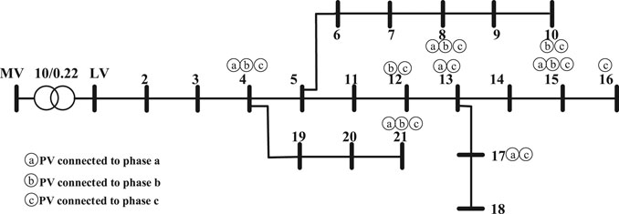
FIGURE 3. Low voltage distribution network with 21 buses.

The power curve of PV is shown in Figure 4A. The value is the per unit value with the peak value to be the base. As the actual power transmission distance of the low-voltage distribution network is short, the conditions such as temperature and light will not be much different. The typical daily photovoltaic power curves connected to each node are hence similar. A typical daily load curve is shown in Figure 4B which is also per unit value. The per unit value of the typical load curves at each bus are similar. For details of the PV and load base data of each node.

FIGURE 4

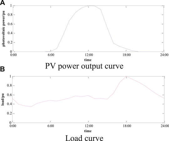
FIGURE 4. Typical daily power curves. (A) PV power output curve. (B) Load curve.

Enhancement in Voltage Violation, Network Loss and Three-phase Unbalance

The effectiveness of the control method in this paper is verified by comparing the calculation results of various indicators of the distribution network with “without control” and “under control”.

(1) Voltage comparison

As the load at phase b is higher than other two phases and the PV integration at phase b is the highest, phase b is taken as an example to compare the voltage with and without the control. See Figure 5 for the simulation results. The blue bar indicates the voltage before the control. When the photovoltaic power generation is high during the day, the loads are at the low consumption period and the voltage exceeds the upper limit. This will lead to reverse power flow and three-phase unbalance. In the evening, there is no power output from photovoltaics, and loads are at the peak consumption period. The voltage is lower than the lower limit. The timing mismatch between photovoltaics and loads results in a higher voltage during the day and a lower voltage in the evening. The red bar indicates the proposed control scheme, and it can be seen that the voltage violation can be effectively suppressed. When the daytime voltage exceeds the upper limit, the photovoltaic inverter absorbs reactive power and suppresses the voltage violation. When the inverter reactive power is insufficient, the energy storage is charged, and the voltage is maintained through the coordinated control of the photovoltaic inverter and energy storage. The voltage is controlled within 1.07 pu. This can not only make up for the shortcomings of exceeding the inverter's reactive power margin when the voltage exceeds the limit, but also for the shortage that the SOC reaches the limit and cannot further charge or discharge. The cooperative control of the two enables the voltage control to be optimal. In the evening, when the power supply is insufficient, the energy stored in the energy storage during the day is fully utilized to maintain the power grid voltage above 0.9 pu.

(2) Three phase unbalance comparison

FIGURE 5

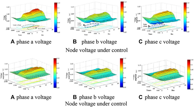
FIGURE 5. Control method under node voltage. Node voltage under control. (A) phase a voltage (B) phase b voltage (C) phase c voltage. Node voltage under control. (A) phase a voltage (B) phase b voltage (C) phase c voltage.

Without the control, as the load is unbalance connected and PV is connected via single phase, this lead to severe three phase unbalance. The unbalance can reach 10.8%. With the control proposed in this paper, all unbalance is limited within 2%. The max value is 0.59% at 12:00. This is because the photovoltaic power generation is sufficient and the load is low, the large-scale single-phase photovoltaic connection leads to the maximum three-phase unbalance. However, the unbalance is still less than the required 2%. Therefore, the proposed control method effectively reduced the three phase unbalance.

(3) Network loss comparison

The total distribution network loss without control is 83.21 kWh. When the upper limit of the voltage during the day or when the lower limit of the voltage during the night, the network loss is the largest in the day. This is because the reverse power flow that occurs when the photovoltaic power is large during the day generates extra network losses in the grid, and the heavy load will increase the network loss in the evening. In addition, the three-phase unbalance caused by the asymmetric connection of photovoltaics and loads causes the neutral line to generate current which further increases the network loss. Under the control scheme, the total network loss is 65.87 kWh, and the network loss is large when the photovoltaic power is large during the day. At the same time, the three-phase unbalance is improved, which reduces the neutral current to zero and further reduces network loss. Therefore, the method proposed in this paper effectively reduces the network loss.

(4) PV and energy storage SOC changes with the proposed control

The PV reactive power at bus 16 is given in Figure 7. As the bus is located at the end of the line, the voltage violation is most likely to occur. Through the proposed scheme, the photovoltaic reactive power is controlled to improve the voltage over-limit and three-phase unbalance. It can be seen that when the upper limit of the voltage during the day is obvious. The photovoltaic absorbs reactive power and mitigate the voltage violation of the upper limit.

FIGURE 6

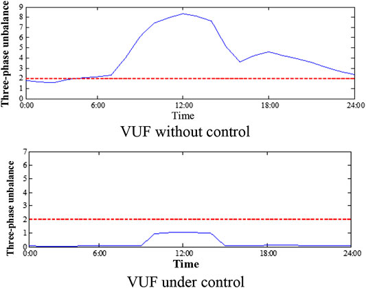
FIGURE 6. Comparison of three–phase imbalances. VUF without control. VUF under control.

FIGURE 7

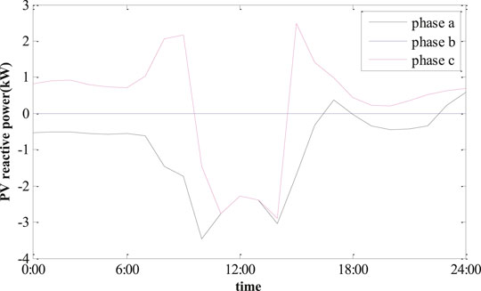
FIGURE 7. PV reactive power under control.

Figure 8 shows the energy storage charging and discharging power at bus 13. As the bus is located at the end of the line, it is also the point where the voltage violation is most likely to occur. In the daytime, excess energy is used to charge energy storage. In the evening, when demand for electricity is high, energy storage is discharged to supply the demand.

FIGURE 8

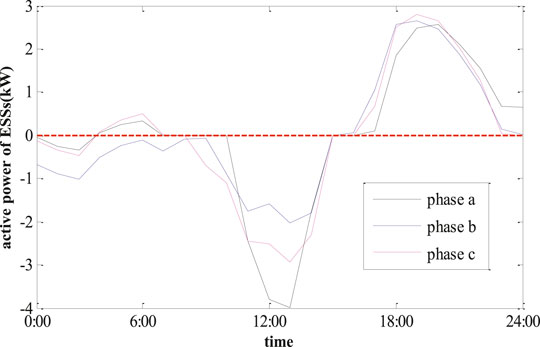
FIGURE 8. Active power of ESSs under control.

Figure 9 shows the changes of the energy storage SOC at bus 13. Around 10:00, photovoltaic power generation continues to increase with the increase in light intensity. At this time, the load is the minimum value throughout the day. The energy storage starts to enter into the charging state, and SOC continues to increase from 20%. At around 15:00, the energy storage reaches the maximum energy limit at 80%. At the time of sunset, following the decrease in light intensity, the power from PV inverter continuously decreases while loads start to increase to peak demand period. Energy storage starts to discharge to supply the load. SOC starts to drop until reaching the low energy limit at 20%. This will not affect the action of energy storage in the next cycle.

FIGURE 9

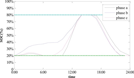
FIGURE 9. SOC of ESSs under control.

Results Comparison of Different Control Method

The target weight indicates the importance of each index in the objective function. Hence, the control performance is related to the value of the weight. Among the three objective functions in the model, the network losses and three-phase unbalance factor are the most important. In this section, the weight of the voltage deviation is always maintained at 0. The control performance with different weights of network losses and three-phase unbalance factor is analyzed. Figure 9 lists the control results of different weighting schemes.

It can be seen from the results that the variation of the voltage deviation in the objective function has a very small influence on the results, almost no change, so the weight of the voltage deviation can be ignored here, and the influence of the network loss and the weight of the three-phase imbalance on the results can be analyzed. The following conclusions are drawn.

(1) Only the three-phase unbalance index is considered. At this time, the distribution network three-phase unbalance control effect is the optimal, reaching a minimum value of 0.52%. However, the network loss is extremely deteriorated, reaching a maximum value of 78.31 kWh.

(2) When the network loss weight is 0.05 and the three-phase unbalance weight is 0.9, the weight is only adjusted slightly. The network loss index changes dramatically. Although the network loss is much smaller, the three-phase unbalance is still 0.52%.

(3) The network loss weight is further increased, and the three-phase unbalance weight is further smaller. The network loss is slightly decreased but not obvious, and the three-phase unbalance is 0.52%. When the three-phase unbalance weight reduce to 0.1, only minor changes can be seen, however still within the national standard (2%).

(4) Consider only the network loss index. Although the network loss can reach a minimum value of 45.77 kWh, the control effect on the three-phase unbalance of the network is not obvious. At this time, the three-phase unbalance is 9.48%, which is far beyond the specified 2%.

In summary, on the premise that the network loss and the three-phase unbalance are within the national standard range, the reasonable weight value is determined based on the principle that the three-phase unbalance and the network loss are not significantly increased. This can ensure the security of the power grid operation and also reduce the operating cost of the power grid. Hence, the three-phase unbalance index takes less weight.

Three-phase Three-Wire and Three-phase Four-Wire System Model Simulation Comparison

In order to verify the superiority of the control method proposed in this paper, a three-phase three-wire system using a second-order cone relaxation solution and a three-phase four-wire system based on OPF proposed in this paper are compared and analyzed. As the second-order cone optimization model cannot calculate the three-phase unbalance, the results of this method are compared with the results of the second-order cone model based on the three-phase three-wire system.

As can be seen from Table 2, compared with the three-phase three-wire system and the three-phase four-wire system, the total network loss differs by 3.41 kWh and the three-phase four-wire neutral line loss is 4.07 kWh. Under the same simulation condition, the difference between the total network losses of the two types of distribution network is approximately equal to the neutral line loss. In addition, the losses of each phase of the two models are quite different. For example, loss of a-phase of the three-phase three-wire system is 15.84 kWh, while the loss of a-phase of the three-phase four-wire system is 18.79 kWh. At this time, the network loss and voltage deviation of three-phase three-wire system has high errors. Therefore, in a three-phase balanced low-voltage distribution network, the neutral line has no current. The two types of distribution networks can be approximately equivalent. For a three-phase unbalanced low-voltage distribution network, the calculation of a three-phase three-wire system will produce errors.

TABLE 1

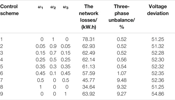
TABLE 1. Result under different strategies.

TABLE 2

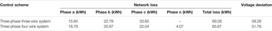
TABLE 2. Result under different line structure.

Conclusion

In this paper, the problems of large-scale domestic photovoltaic connecting to the three-phase four-wire low-voltage distribution network including voltage violation and three-phase unbalance were studied. A low-voltage photovoltaic-energy storage based on the three-phase four-wire network OPF cooperative control method is proposed.

(1) For a low-voltage distribution network with a high proportion of photovoltaics, the proposed photovoltaic-energy storage collaborative control method can comprehensively improve the technical indicators of the power grid. The node voltage can be controlled within the range of 0.9–1.07 pu, and also effectively reduce the three-phase unbalance and the network loss.

(2) The proposed three-phase four-wire optimal power flow algorithm overcomes the shortcomings that the existing method that cannot accurately calculate the neutral line voltage and current. This ensures the correctness of the network optimization calculation results in the case of three-phase unbalance. It has good adaptability to low-voltage distribution network.

(3) In the objective function, the network loss, the three-phase unbalance and the voltage deviation weight have different effects on the control results. The network loss weight is more sensitive to the objective function than the three-phase unbalance and the voltage deviation. The control effect is better when the network loss weight is set in the range of 0.7–0.9.

Data Availability Statement

The original contributions presented in the study are included in the article/Supplementary Material, further inquiries can be directed to the corresponding author.

Author Contributions

The paper was a collaborative effort between the authors. JF designed the coordinated control model, TL contributed to the Introduction, SG and YW contributed to the multi-state models of REG active power considering forecast errors, KT and YD contributed to case study.

Funding

This research was funded by Beijing Key Laboratory of Distribution Transformer Energy-Saving Technology (China Electric Power Research Institute), grant number 51201901230.

Conflict of Interest

The authors declare that the research was conducted in the absence of any commercial or financial relationships that could be construed as a potential conflict of interest.

Appendix

TABLE A1

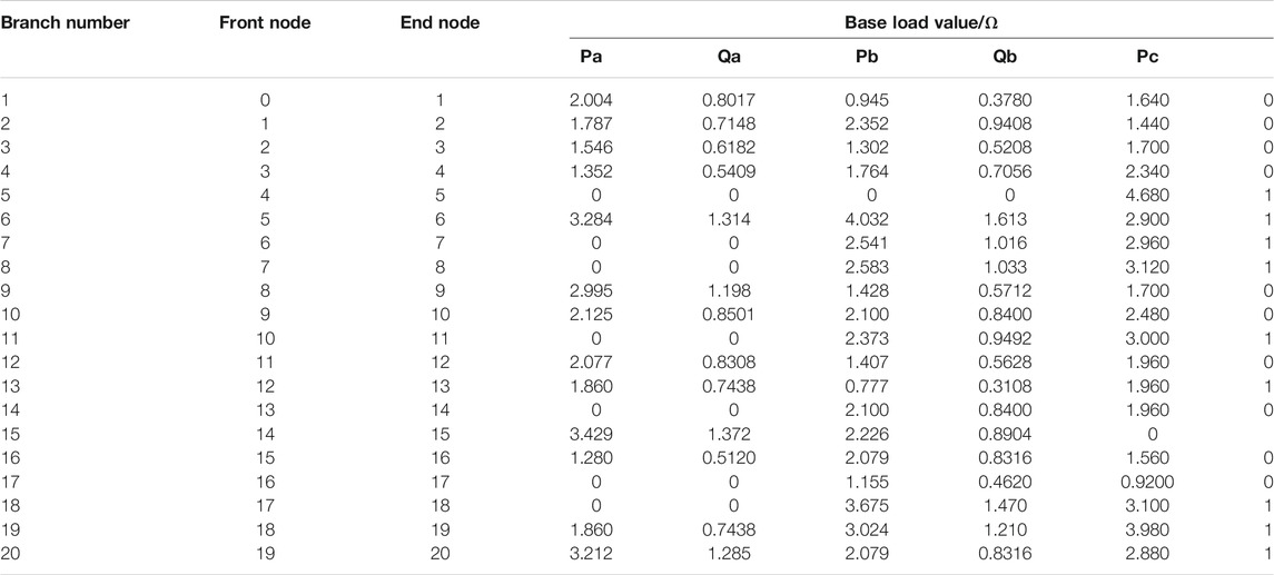
TABLE A1. Three-phase four-wire 21-bus test system.

References

Alsenani, T. R., and Paudyal, S. (2018). “Distributed approach for solving optimal power flow problems in three-phase unbalanced distribution networks,” in 2018 Australasian universities power engineering conference (AUPEC), Auckland, NZ, November 29–30, 2018 (IEEE), 1–6.

Google Scholar

Aziz, T., and Ketjoy, N. (2017). PV penetration limits in low voltage networks and voltage variations. IEEE Access 5 (99), 1. doi:10.1109/ACCESS.2017.2747086

CrossRef Full Text | Google Scholar

Bose, A., Tian, Z., Wu, W., and Zhang, B. (2016). Mixed-integer second-order cone programing model for VAR optimisation and network reconfiguration in active distribution networks. IET Gener. Transm. Distrib. 10 (8), 1938–1946. doi:10.1049/iet-gtd.2015.1228

CrossRef Full Text | Google Scholar

Bozchalui, M., and Sharma, R. (2014). Optimal operation of energy storage in distribution systems with renewable energy resources. 2014 Clemson university power systems conference, Clemson, SC, March 11–14, 2014 (IEEE).

CrossRef Full Text | Google Scholar

Gill, S., Kockar, I., and Ault, G. (2014). Dynamic optimal power flow for active distribution networks. IEEE Trans. Power Syst. 29 (1), 121–131. doi:10.1109/TPWRS.2013.2279263

CrossRef Full Text | Google Scholar

Ju, Y., Wu, W., Lin, Y., Ye, L., and Ge, F. (2017). Three-phase optimal load flow model and algorithm for active distribution networks. 2017 IEEE Power and energy society general meeting, Chicagol, IL, July 16–20, 2017 (IEEE), 1–5.

Google Scholar

Liu, X., Aichhorn, A., Liu, J., and Li, H. (2012). Coordinated control of distributed energy storage system with tap changer transformers for voltage rise mitigation under high photovoltaic penetration. IEEE Trans. Smart Grid 3 (2), 897–906. doi:10.1109/TSG.2011.2177501

CrossRef Full Text | Google Scholar

Martins, V. F., and Carmenlt, L. T. B. (2011). Active distribution network integrated planning incorporating distributed generation and load response uncertainties. IEEE Trans. Power Syst. 26 (4), 2164–2172. doi:10.1109/TPWRS.2011.2122347

CrossRef Full Text | Google Scholar

Niknam, T., Narimani, M. R., Aghaei, J., and Azizipanah-Abarghooee, R. (2012). Improved particle swarm optimisation for multi-objective optimal power flow considering the cost, loss, emission and voltage stability index. IET Gener. Transm. Distrib. 6 (6), 515–527. doi:10.1049/iet-gtd.2011.0851

CrossRef Full Text | Google Scholar

O’Neill, R. P., Castillo, A., and Cain, M. (2012). The IV formulation and linear approximations of the AC optimal power flow problem. Washington, DC: Federal Energy Regulation Commission Staff Tech. Paper.

Google Scholar

Pansakul, C., and Hongesombut, K. (2014). Analysis of voltage unbalance due to rooftop PV in low voltage residential distribution system. 2014 International electrical engineering congress (iEECON), Chonburi, Thailand, March 19–21, 2014 (IEEE).

CrossRef Full Text | Google Scholar

Qian, M., Qin, H., Zhao, D., Chen, N., Jiang, J., Wang, B., et al. (2018). A multi-level reactive power control strategy for PV power plant based on sensitivity analysis. 2018 China international conference on electricity distribution (CICED), Tianjin, China, September 17–19, 2018 (IEEE), 1838–1842.

Google Scholar

Reinaldo, T., Lopes, L., and Tarekhm, H. M. E.-F. (2011). Coordinated active power curtailment of grid connected PV inverters for overvoltage prevention. IEEE Trans. Sustain. Energy 2 (2), 139–147. doi:10.1109/TSTE.2010.2098483

CrossRef Full Text | Google Scholar

Tian, Z., Wu, W., Zhang, B., and Bose, A. (2016). Mixed-integer second-order cone programing model for VAR optimisation and network reconfiguration in active distribution networks. IET Gener. Transm. Distrib. 10 (8), 1938–1946. doi:10.1049/iet-gtd.2015.1228

CrossRef Full Text | Google Scholar

Tonkoski, L. (2009). Voltage regulation in radial distribution feeders with high penetration of photovoltaic. 2009 IEEE energy 2030 conference, Atlanta, GA, September 1–7, 2009 (IEEE).

Google Scholar

Zafar, R., Ravishankar, J., Fletcher, J. E., and Pota, H. R. (2020). Optimal dispatch of battery energy storage system using convex relaxations in unbalanced distribution grids. IEEE Trans. Indust. Inform. 16 (1), 97–108. doi:10.1109/TII.2019.2912925

CrossRef Full Text | Google Scholar

Zehar, K., and Sayah, S. (2008). Optimal power flow with environmental constraint using a fast successive linear programming algorithm: application to the algerian power system. Energy Convers. Manag. 49 (11), 3362–3366. doi:10.1016/j.enconman.2007.10.033

CrossRef Full Text | Google Scholar

Zhang, B., Tang, W., Cai, Y., Wang, Z., Li, T., and Zhang, H. (2020). Distributed control strategy of residential photovoltaic inverter and energy storage based on consensus algorithm. Auto. Elect. Power Syst. 44 (02), 86–96. doi:10.7500/AEPS20190305005

CrossRef Full Text | Google Scholar