Robust Scheduling for Networked Microgrids Under Uncertainty

1. Introduction

Conventionally, power systems contain a few large-scale generation facilities that supply energy to the passive loads. Lately, this arrangement has been slowly transforming into a multi-layered, cyber-physical intelligent grid with active loads and small-scale generators. These small-scale generators based on intermittent renewable sources are presently not involved in grid operations and the major concerns for rejecting their participation often include the small size and unreliability of Distributed Generatorss (DGs) (Saraiva and Gomes, 2010). By using the concept of a Microgrid (MG), the DGs and aggregated Flexible Loads (FLs) can be clustered to form larger market players and provide ancillary services (Guerrero et al., 2013). The MGs can either be connected to the main grid or be interconnected to form a networked-MG system (Figure 1), where the new decentralized structure contributes to establishing a competitive market and benefits the social welfare of the underlying system. Some practical examples include the networked MGs on the campus of the Illinois Institute of Technology and its adjacent community Bronzeville (Shahidehpour et al., 2017), where the optimal energy management mechanisms for interconnected MGs are exploited.

FIGURE 1

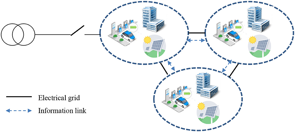
Figure 1. System overview.

The networked MG system is different from the traditional power distribution grid, because the power flow is bidirectional from one MG to another MG or to the distribution grid. The change in network topology can be frequent in networked MGs. If implemented and managed properly, networked MGs can provide a variety of benefits to electric power utilities and consumers in terms of supply efficiency, security, and reliability (Alam et al., 2019). In the scope of their market participation, the literature proposes the networked MGs participate in the local Distribution System Operator (DSO) market (Hirsch et al., 2018; Alam et al., 2019), wherein the networked MG system can act as virtual power plant with each MG's controller having direct control over its resources. In regard to this, MGs can be owned by utilities, end customers, or consortia of prosumers. For the latter cases that the Distributed Energy Resourcess (DERs) are not the assets of the MG, direct control of these assets might not be easily exercised in the context of a deregulated market. To this end, the indirect control over DERs can be achieved by the introduction of a virtual layers of Mirogrid Operator (MGO)s. Each MG is assumed to be managed by the local MGO that is an independent entity to collect the local prosumers' bids from FLs, and DGs and to coordinate with the market of the external power system to provide energy and ancillary services. With the networked MGs geographically scattered over multiple communities, the network constraints of the networked MGs can be respected at the same time.

1.1. Related Work and Contributions

For the market integration of networked MGs under the transactive energy paradigm (Rahimi et al., 2016), Sabounchi and Wei (2017) propose a block-chain based mechanism to enable the electricity exchange for energy prosumers in an networked MG system environment, where actual grid operation challenges for networked MGs remain undiscussed. Various studies (Wang et al., 2015; Wu et al., 2019) propose a bi-level-programming model for the MGs' bidding strategy in the distribution grid market based on the assumption that the prosumers have full knowledge of the distribution grid information, such as topology and loading profile. This may be unrealistic for some countries where the grid information is considered to be confidential (see, e.g., Trpovski et al., 2018). To this end, market design and frameworks for networked MGs can be developed by considering the statistical distribution of available data, such as the market-clearing prices and its underlying uncertainty (e.g., Kim and Poor, 2011). Various approaches including stochastic programming, chance-constrained models, robust optimization, and distributionally robust optimization exist in the literature to develop the optimal exchange framework for the networked MG operation in coordination with the main grid.

Chance-constrained models are employed to tackle the uncertainties for the networked MG scheduling problem in works (Bazmohammadi et al., 2018, 2019a,b; Daneshvar et al., 2020a), where Gaussian distribution and beta distribution are assumed to describe the uncertain parameters for electricity prices and Photovoltaics (PV) generation to relax the chance constraints while ensuring that the problem is numerically tractable. From a practical perspective, the exact distribution of uncertain variables is difficult to obtain for given empirical data as we later demonstrate in a case study for electricity prices and load profile, where machine learning-based approaches may deliver a better estimation for these uncertainties. To remove this drawback, the sampling technique can be adopted to transform the chance-constrained model to stochastic programming problems, where it provides an alternative way to handle uncertainties by generating discrete probabilistic scenarios of the uncertain parameter and integrating them into the optimization problems (see, e.g., Weron, 2005; Daneshvar et al., 2020b). Though this approach does not rely on specific types of distribution, both the solution quality and computational efficiency can be highly impacted by the scenarios that are utilized in the problem formulation. Similar to stochastic programming, another approach that does not rely on the exact knowledge of the distribution of uncertain parameters is robust optimization. Instead of optimizing the expected objective value as in stochastic programming, robust optimization essentially provides a conservative solution by considering the worst-case scenario realization of the stochastic parameters that are modeled with continuous uncertainty sets. This, on the one hand, may require less computational power, but, on the other hand, leads to a conservative solution by considering the worst-case scenario. It is worth pointing out that robust optimization based solution methodologies allow the tuning of conservatism parameters to reflect the attitude of energy prosumers. Some examples are shown in Wang et al. (2015) and Correa-Florez et al. (2020), where robust optimization for load aggregation in a DSO market and DG generation for single MG operation are proposed, respectively.

In the center of the solution methodology design for networked MGs operation, an important aspect is the operational autonomy. Networked MGs naturally have a decentralized operation structure, where the ownership of the MGs can vary, being utility-owned, customer-owned, or third-party operated MGs (Alam et al., 2019). Centralized approaches for managing the networked MGs require each MG operator to reveal their complete local system information to a central entity, which may introduce both privacy and scalability concerns in the system. A large body of existing literature has focused on a centralized dispatch model (e.g., Bazmohammadi et al., 2019a; Daneshvar et al., 2020a; among others). In contrast, with a decentralized operation structure, competition can be introduced between the MGs to establish a competitive market at the distribution-grid level. A recent exposition (Liu et al., 2020) uses a bi-level model for the market-clearing purpose between DSO and networked MGs, where bi-level optimization models introduce two hierarchical levels to regulate the market-clearing procedure. In this work, we focus on the interconnected MGs exchange problem, wherein the distribution network is clustered into MGs with a plain operation structure for the MGOs. For this structure, decomposition methods can be applied (Zhang et al., 2020). There are some works considering the decomposition method for the networked MG management problem. For example, Ma et al. (2018) proposes an online Alternating Direction Method of Multipliers (ADMM)-based algorithm to handle real-time dispatch problems for networked MGs. Work by Liu et al. (2017) proposes the decomposition methods for deterministic day-ahead networked MGs scheduling. Although these works concentrate on the decomposable operation structure to preserve information privacy, the uncertainty handling for day-ahead trading within networked MGs has not been addressed yet.

In view of the existing works and research gap, we focus in this work on the day-ahead energy exchange problem for networked MGs considering the grid constraints and the uncertain parameters preserving a decentralized Peer-to-peer (P2P) operation structure. In terms of essential solution methodology choices, we use the combination of the ADMM-based decomposition method and robust optimization. The reasons are 3-fold. First, ADMM is well-suited to distributed optimization and large-scale distributed computing systems. By using ADMM, we do not need to have a centralized computation center and the computation can be distributed across the MG operators. Specifically, ADMM consists of several inner loop subroutines that can be assigned to each MG operator. Each subroutine is an optimization problem that can be solved in a parallel and independent fashion. Second, ADMM can be interpreted as a form of tâtonement process, which essentially adjusts the prices to achieve the market equilibrium, following the Walras theory of general equilibrium (Boyd et al., 2011). This plays an essential part in the market design for the networked MGs. Third, the combination of robust optimization and ADMM allows individual parameter settings by each MGO to set their conservatism, avoiding an over-conservative solution based on their preference. Moreover, full operational autonomy is ensured with only information regarding the selling/buying quantity exchanged. Despite the different estimation of uncertainties and conservatism parameter settings, given the solution feasibility, a unique market equilibrium can be attained.

The main contributions of this work are summarized as follows:

• To enable fully decentralized operation, we propose an ADMM-structured robust optimization method for the networked MG energy exchange problem, while maintaining the autonomy and robustness of the decentralized grid organization considering local MG contingencies (e.g., congestion between MGs). The combination of robust optimization and ADMM allows individual parameter settings by each MGO, ensuring full operational autonomy with only information regarding the selling/buying quantity exchanged. It also enables individual parameter settings of each MGO to set their conservatism, avoiding an over-conservative solution.

• The market equilibrium is derived for the energy exchange prices between MGs under different grid conditions, whereas the heterogeneous preferences for parameter settings for MGOs in robust optimization are exploited to analyze the impact on the equilibrium point.

The paper is structured as follows. In section 2, we provide the modeling choices for DER assets, networked MGs, grid models including voltage and line flows, and the uncertainty models. In section 3, both the deterministic and robust form for the networked MG energy exchange problem is described. The ADMM-structured robust optimization solution methodology is presented in section 4. In particular, we analyze the market equilibrium using the exchange price decomposition in section 4.2. Finally, the simulation results and case studies for different grid conditions and parameter settings are presented in section 5. Section 6 summarizes this work with observations and outlook.

2. System Modeling

2.1. Networked MG System

In this work, we focus on the networked MG system, where each MG is assumed to be operated by a MGO. MGOs are supposed to be independent entities for coordinating, controlling, and monitoring the local MG system. They obtain buying and selling bids from the local prosumers (small-scale generators, FLs) and can coordinate with other MGOs in the same networked MG system. The networked MG system can also exchange electricity through Power Common Coupling (PCC) with the main grid. The collective objective of the networked MG system is to minimize the total MG operational cost. First, local prosumers submit their bids to the respective MGOs. Second, the welfare maximization problem of networked MGs is solved by all MGOs using the proposed distributed algorithm with information exchange regarding proxy variables of power exchange quantity. The energy exchange schedule and market-clearing prices of the networked MG are determined during the market clearing.

2.2. Distributed Energy Resource

We assume a generic energy prosumer model for DERs that manages the optimal set points of its assets, i.e., generators, energy storage, and loads. To this end, the DERs are categorized into (i) DGs with active/reactive power injection capabilities and (ii) FLs with flexible active power consumption capabilities. All market participants are assumed to be economically rational, hence they seek the maximization of their individual economic surplus. The prosumer nodes are labeled as DGs and FLs and described by set $\mathcal{G}:=\left\{1,2,...,g\right\}$ for the DGs and $\mathcal{F}:=\left\{1,2,...,fl\right\}$ for the FLs. The set $\mathcal{T}:=\left\{1,2,...,T\right\}$ is defined to include all the market intervals.

2.2.1. DER Model

For DERs, the electric power injection or consumption is limited by the system constraints, e.g., the curtailment capacity of a commercial building is limited by the comfort of its occupants; the reactive power injection of a DG is limited by the inverter capacity. Such system constraints are expressed with as box constraints:

$\begin{array}{ll}{\underset{\_}{\text{p}}}_t^{\text{x}}\le {\text{p}}_t^{\text{x}}\le {\overline{\text{p}}}_t^{\text{x}},\text{ x}\in \{\text{g},\text{fl}\},t\in \mathcal{T}& (1)\end{array}$

$\begin{array}{ll}{\underset{\_}{\text{q}}}_t^{\text{x}}\le {\text{q}}_t^{\text{x}}\le {\overline{\text{q}}}_t^{\text{x}},\text{ x}\in \{\text{g}\},t\in \mathcal{T}.& (2)\end{array}$

DERs within a MG are assumed to form their bids based on the cost function and the system constraints and submit the bids to the local MGO. MGs are assumed to be equipped with Battery Energy Storage Systems (BESSs). Let set $\mathcal{B}:=\left\{1,2,...,b\right\}$ contain the BESSs in all MGs and ${\text{soc}}_t\in {ℝ}^b$ denote the State of Charge (SOC) of the BESSs at time step t. Q ∈ ℝ^b is used represent the battery capacity and p^d, p^ch ∈ ℝ^b denote the discharge and charge power. SOC of BESSs is described with a linearized model:

$\begin{array}{ll}{\text{soc}}_t={\text{soc}}_0-{\text{diag}}^{-1}(\text{Q}){\displaystyle \sum _{k=1}^t}(\frac{1}{{\eta }^d}{\text{p}}_k^{\text{d}}-{\eta }^c{\text{p}}_k^{\text{c}})\text{Δ}t& (3)\end{array}$

where η^c, η^d ∈ ℝ represent the charge and discharge efficiency and Δt represents the market period duration. Hence, the nodal injections of BESS at time t from is given as ${\text{p}}_t^{\mathrm{\text{b}}}={\text{p}}_t^{\mathrm{\text{d}}}-{\text{p}}_t^{\mathrm{\text{c}}}\in {ℝ}^b$.

2.2.2. Cost Function

It is further assumed that the cost for each MGO to procure electric power generation/load curtailment from the DERs can be expressed with a quadratic function

$\begin{array}{ll}{C}_t^{\text{x}}({\text{p}}_t^{\text{x}})=({\text{c}}_t^{\text{x}}+\text{diag}({\text{d}}_t^{\text{x}})·{\text{p}}_t^{\text{x}}{)}^{⊺}·{\text{p}}_t^{\text{x}},\text{x}\in \left\{\text{g},\text{fl}\right\},t\in \mathcal{T}& (4)\end{array}$

where p^x ≥ 0 ∈ ℝ^x is the electric power injection or consumption and c^x, d^x are the coefficients for the linear and quadratic terms. The quadratic cost function is strictly convex with zero-crossing. The bid formulation for all the DER types is summarized in Figure 2. For example, the FL bid consists of a baseline load ${\underset{\_}{p}}_t^{\mathrm{\text{fl}}}$ and a price-sensitive part $\left[{\underset{\_}{\text{p}}}_t^{\mathrm{\text{fl}}},{\overline{\text{p}}}_t^{\mathrm{\text{fl}}}\right]$ with the marginal cost ${\text{c}}_t^{\mathrm{\text{fl}}}+\mathrm{\text{diag}}({\text{d}}_t^{\mathrm{\text{fl}}})·{\text{p}}_t^{\mathrm{\text{fl}}}$ representing their willingness to be curtailed in dependence with the market-clearing price.

FIGURE 2

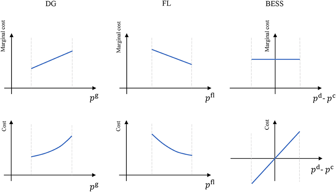
Figure 2. Bid formulation and cost function for DGs, FLs, and BESSs.

For batteries, the rational behind the price sensitivity is to capture the battery aging effect from the charging and discharging process. Interested readers are encouraged to refer to Liu et al. (2017) for the derivation of the parameter settings for batteries, which gives a quadratic cost function:

$\begin{array}{ll}{C}_t^{\text{b}}({\text{p}}_t^{\text{d}},{\text{p}}_t^{\text{c}})=({\text{p}}_t^{\text{d}}+{\text{p}}_t^{\text{c}}{)}^{⊺}\text{diag}({\text{d}}_t^{\text{b}})({\text{p}}_t^{\text{d}}+{\text{p}}_t^{\text{c}}),& (5)\end{array}$

with ${\text{d}}_t^{\mathrm{\text{b}}}\in {ℝ}^{b_i}$ giving the price vector for the charge/discharge in each MG. This formulation also prevents the simultaneous charging and discharging of the BESSs when the system operator (e.g., MGO) solves the optimization problem. Intuitively speaking, any optimal solution to minimize Equation (5) will always assign one of the variables ${\text{p}}_t^{\mathrm{\text{c}}},{\text{p}}_t^{\mathrm{\text{d}}}$ to be zero to avoid additional cost.

2.3. Grid Model

Consider the networked MG system in Figure 1; we assume the individual MGs can be considered as a portion of a low-voltage (LV) distribution grid with a reference node indexed by 0. In the grid-connected mode, the MG is connected to the distribution grid via PCC, where the reference is modeled as a slack node with fixed voltage. The rest of the nodes are modeled as PQ nodes. All MG nodes are included in set $\mathcal{N}:=\left\{0,1,2,\dots ,n\right\}$. In addition, we define the set $\mathcal{H}:=\left\{1,2,\dots ,h\right\}$ containing all the lines connecting the nodes. Let set $\mathcal{M}\mathcal{G}:=\left\{1,2,\dots ,mg\right\}$ denote the set of all MGs, and we obtain for MG $i\in \mathcal{M}\mathcal{G}$ the regional version of its respective nodes set and lines set as ${\mathcal{N}}_i:=\left\{0_i,1_i,2_i,\dots ,n_i\right\},{\mathcal{H}}_i:=\left\{1_i,2_i,\dots ,h_i\right\}$, where $\mathcal{N}:={\bigcup }_{i\in \mathcal{M}\mathcal{G}}{\mathcal{N}}_i$ and $\mathcal{H}:={\bigcup }_{i\text{∈}\mathcal{M}\mathcal{G}}{\mathcal{H}}_i$. All the local DGs/FLs in MG $i\text{∈}\mathcal{M}\mathcal{G}$ are included in set ${\mathcal{G}}_i:=\left\{1_i,2_i,\dots ,g_i\right\},{\mathcal{F}}_i:=\left\{1_i,2_i,\dots ,f{l}_i\right\}$, where $\mathcal{G}:={\bigcup }_{i\text{∈}\mathcal{M}\mathcal{G}}{\mathcal{G}}_i$ and $\mathcal{F}:={\bigcup }_{i\text{∈}\mathcal{M}\mathcal{G}}{\mathcal{F}}_i$.

2.3.1. Linearized Nodal Injection Model

The complex nodal injections and voltages are, respectively, represented for all nodes as s : = p + ȷq and u : = v · e^ȷθ all with dimension ℂⁿ⁺¹. The individual node $i\in \mathcal{N}$ defines s_i : = p_i + ȷq_i and $u_i=v_i{e}^{ȷ{\theta }_i}$. The overall grid is modeled using the admittance matrix $\text{Y}:={\{y_{ij}\}}_{1\text{≤}i,j\text{≤}n\text{+}1}\in {ℂ}^{(n\text{+}1)\text{×}(n\text{+}1)}$ with its regional version for MG $i\in \mathcal{M}\mathcal{G}$ denoted by ${\text{Y}}_i\in {ℂ}^{(n_i\text{+}1)\text{×}(n_i\text{+}1)}$. Considering only PQ (constant power) nodes exist in the grid, we have the nodal injection model at each time step $t\in \mathcal{T}$ (Bolognani and Dörfler, 2015):

$\begin{array}{ll}{\text{s}}_t={\text{p}}_t+ȷ{\text{q}}_t=\text{diag}({\text{u}}_t)\underset{\_}{\text{Y}}{\underset{\_}{\text{u}}}_t& (6)\end{array}$

The nodal injection model is complex and non-linear. We adapt the first-order linearization for eq. (6) as in Bolognani and Dörfler (2015, Proposition 1). It assumes that the nodal angle differences are very small throughout the network, so the flat voltage, i.e., θ ≈ 0, v ≈ 1, is used as the linearization point. We obtain the following linearized power injection model (Linearized DistFlow Model) (Farivar et al., 2013).

$\begin{array}{ll}\left[\begin{array}{c}{\text{p}}_t\\ {\text{q}}_t\end{array}\right]=\left[\begin{array}{cc}\Re (\text{Y})& -\Im (\text{Y})\\ -\Im (\text{Y})& -\Re (\text{Y})\end{array}\right]\left[\begin{array}{c}{\text{v}}_t\\ {\theta }_t\end{array}\right].& (7)\end{array}$

Note that the approximation based on Linearized DistFlow has been shown to perform reasonably well in voltage estimation [0.25% error for 5% voltage variation from the nominal voltage (Farivar et al., 2013)] while neglecting the higher order active/reactive loss terms. For the operation of geographically closed networked-MGs, the aim is to minimize the overall operating cost, without focusing on the losses that are small compared to the amount of energy exchange among the MGs.

2.3.2. Linearized Line Current Model

To constrain the line flow so as not to exceed the thermal limit, we consider the following linearized line current model. Defining the line current between node i and node j as l_ij ∈ ℂ, thermal limits are usually defined as the line current magnitude |l_ij|, which is directly related to the conductor's temperature. For brevity, we obtain the following line current magnitude by assuming no existence of shunt admittance:

$\begin{array}{l}|l_{ij}|=\sqrt{l_{ij}{\underset{\_}{l}}_{ij}}\\ =\sqrt{(u_i-u_j)y_{ij}({\underset{\_}{u}}_i-{\underset{\_}{u}}_j){\underset{\_}{y}}_{ij}}\\ =\sqrt{|y_{ij}{|}^2(v_i^2+v_j^2-v_i{v}_j{e}^{({\theta }_i-{\theta }_j)ȷ}-v_i{v}_j{e}^{({\theta }_j-{\theta }_i)ȷ})}.& (8)\end{array}$

Based on the same assumption of small angle variance, i.e., θ_i − θ _j = 0, we obtain

$\begin{array}{ll}|l_{ij}|=|y_{ij}||v_i-v_j|& (9)\end{array}$

It essentially provides a linear projection from the voltage difference to the line current magnitude. We now rewrite eq. (9) in a compact form using the admittance matrix Y^line ∈ ℂ^h×h and the from/to mapping matrix C^f, C^t ∈ ℝ^h×(n+1). The basic idea of representing in from/to quantities is illustrated in Figure 3, where each line segment is assigned a from/to direction from the start/end node to the end/start node. Hence, C^f/C^t maps each line segment to the corresponding node index (see also Zimmerman, 2020). Y^line is defined as a matrix with its diagonal terms equal to the line admittance and the off-diagonal terms equal 0. We obtain the line current magnitude vector |l| ∈ ℝ^h at time step $t\in \mathcal{T}$ represented as

$\begin{array}{ll}|{\text{l}}_t|=|{\text{Y}}^{\text{line}}\Vert {\text{C}}^{\text{f}}{\text{v}}_t-{\text{C}}^{\text{t}}{\text{v}}_t|,& (10)\end{array}$

where |Y^line| ∈ ℝ^h×h extracts the magnitude of the matrix Y^line. Consider the thermal constraint that $|l|\text{≤}|\overline{l}|;$ an equivalent box constraint at time step $t\in \mathcal{T}$ is obtained as.

$\begin{array}{ll}-|\overline{l}|\le |{\text{Y}}^{\text{line}}|({\text{C}}^{\text{f}}-{\text{C}}^{\text{t}}){\text{v}}_t\le |\overline{l}|& (11)\end{array}$

FIGURE 3

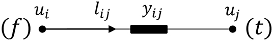
Figure 3. Line current model with a from/to direction.

2.4. Uncertainty Model

Since the networked MG system is exposed to the external electricity market in the main grid, uncertainties in the electricity prices may need to be explicitly considered. For example, the forecast for electricity prices in the Singapore real-time spot market is released 36 h prior to the actual market period. Other uncertainties are from the local MG demand and DG generations, e.g., solar PV generators. These uncertainties need to be explicitly considered and modeled to ensure the robustness of the solution. The motivation for modeling the electricity prices is to have an adequate representation of spot price trends on a weekly and monthly basis, with time resolution consistent with the underlying market periods for the prosumers to decide on their market participation preference. Since the demand and the spot prices are correlated, models for both shall be obtained simultaneously. Note that the renewable generation is neglected in the following. This is because, for the studied data set from Singapore's wholesale market, the renewable injections are still very small compared to the demand. Nevertheless, the renewable generation can be taken into account by following the same procedures as in modeling the demand and their influence on the spot prices.

We adopt a dynamic regression model with Autoregressive-moving-average (ARMA) errors to model demand and price time series. First, the ARMA model for the demand time series is given as

$\begin{array}{ll}{D}_t={\kappa }_t^{\text{D,y}}+{\kappa }_t^{\text{D,m}}+{\kappa }_t^{\text{D,w}}+{\displaystyle \sum _{l\in {\mathcal{L}}_{\text{ARMA}}^{\text{D}}}}({\varphi }_l^{\text{D}}{D}_{t-l}+{\theta }_l^{\text{D}}{ϵ}_{t-l})+{ϵ}_t^{\text{D}}& (12)\end{array}$

The first three terms show the constant components of the load model, representing trends for yearly ${\kappa }_t^y$, monthly ${\kappa }_t^m$, and weekly ${\kappa }_t^w$ cycles. The last three terms are the stochastic components in the ARMA model including a Gaussian-distributed term ${ϵ}_t^D$. Based on the demand model, the price model consists of a deterministic portion and a stochastic portion. The deterministic portion is determined by a linear regression model to represent long-term trends, e.g., seasonality, and the demand's influence on the spot prices. On the other hand, the stochastic component is determined by an ARMA model to represent the underlying evolution of the error terms. The log-transformed spot price model is described as

$\begin{array}{l}\text{log}({\gamma }_{,t})\text{=}{\text{b}}_t^{⊺}\beta +a+{\displaystyle \sum _{l\in {ℒ}_{ARMA}^{\text{c}}}(}{\delta }_l\text{log}(D_{t-l})+{\varphi }_l^{\text{c}}\text{log}({\gamma }_{t-l})\\ +{\theta }_l^{\text{c}}\text{log}({ϵ}_{t-l}))+{ϵ}_t^{\text{c}}& (13)\end{array}$

Herein, b_t is the vector of dummy variables values for the respective time step including a single variable representing the index for the linear trend. Entries of vector β are the corresponding coefficients, estimated by the regression model. Furthermore, a is the offset determined by the regression. Term δ_llog(d_t−l) is the influence of the demand time series, in which coefficient δ_l has been determined by the regression as well. Accordingly, all mentioned terms so far are the deterministic component of the model. In addition, the remaining terms represent the ARMA model, with ${\varphi }_l^{\mathrm{\text{c}}}$ and ${\theta }_l^{\mathrm{\text{c}}}$ being the coefficient of the AR and MA terms, respectively. Finally, ${ϵ}_t^{\mathrm{\text{c}}}$ denotes the error terms of the ARMA model. One example is given for the generated scenarios for electricity prices in Singapore in Figure 4. Similar modeling procedures can be followed for PV generations (see also Huang et al., 2012).

FIGURE 4

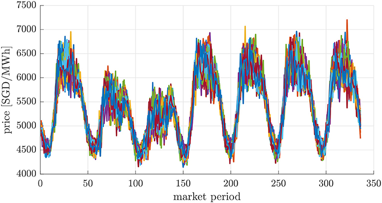
Figure 4. Example of scenarios generation for the ARMA electricity price model in Singapore.

Based on the demand model in eq. (12) and the spot pricing model in eq. (13), we need to obtain the lower and upper bound for these uncertain quantities. To this end, to achieve a suitable representation of the uncertainty, a high number of scenarios are needed, which are generated using Monte Carlo simulation. The upper and lower bound of the confidence interval can be used to bound the uncertain price sequences by accessing the generated scenarios, where

$\begin{array}{ll}{\gamma }_t^{\text{mean}}-{\widehat{\gamma }}_t^{-}\le {\gamma }_t\le {\gamma }_t^{\text{mean}}+{\widehat{\gamma }}_t^{+},& (14)\end{array}$

where ${\widehat{\gamma }}_t^{+,-}$ is the maximal allowed deviation to the estimated value given a predefined confidence level.

3. Networked Microgrid Operation Under Uncertainty

Since the MGs are interconnected, each MG has the coupled nodes shared with other MGs to exchange power. All the coupled nodes for MG i are included in set ${\mathcal{M}}_i:=\left\{1_i,2_i,\dots m_i\right\}\in {ℝ}^{m_i}$. Furthermore, the power exchange vectors ${\text{p}}_{i,t}^{\mathrm{\text{exc}}},{\text{q}}_{i,t}^{\mathrm{\text{exc}}}\in {ℝ}^{m_i}$ are associated with the coupled nodes. Hence, the nodal injections ${\text{p}}_{i,t},{\text{q}}_{i,t}\in {ℝ}^{n_i\text{+}1}$ in MG i are the total of the electricity withdrawn from the distribution grid $p_i^{\mathrm{\text{pcc}}}$, DG injections ${\text{p}}_{i,t}^{\mathrm{\text{g}}},{\text{q}}_{i,t}^{\mathrm{\text{g}}}\in {ℝ}^{g_i}$, energy exchange ${\text{p}}_{i,t}^{\mathrm{\text{exc}}}\in {ℝ}^{m_i}$ and flexible/non-elastic loads ${\text{p}}^{\mathrm{\text{fl}}}\in {ℝ}^{f{l}_i},{\text{p}}^{\mathrm{\text{D}}},{\text{q}}^{\mathrm{\text{D}}}\in {ℝ}^{n_i\text{+}1}$. It is obtained as

$\begin{array}{l}{\text{p}}_{i,t}={\text{a}}_i^{\text{pcc}}{p}_{i,t}^{\text{pcc}}+{\text{A}}_i^{\text{g}}{\text{p}}_{i,t}^{\text{g}}+{\text{A}}_i^{\text{b}}({\text{p}}_{i,t}^{\text{d}}-{\text{p}}_{i,t}^{\text{c}})+{\text{A}}_i^{\text{exc}}{\text{p}}_{i,t}^{\text{exc}}-{\text{A}}_i^{\text{fl}}{\text{p}}_{i,t}^{\text{fl}}\\ \begin{array}{l}-{\text{p}}_{i,t}^{\text{D}}\end{array}& (15)\end{array}$

$\begin{array}{ll}{\text{q}}_{i,t}={\text{a}}_i^{\text{pcc}}{q}_{i,t}^{\text{pcc}}+{\text{A}}_i^{\text{g}}{\text{q}}_{i,t}^{\text{g}}+{\text{A}}_i^{\text{exc}}{\text{q}}_{i,t}^{\text{exc}}-{\text{q}}_{i,t}^{\text{D}},& (16)\end{array}$

where ${\text{a}}_i^{\mathrm{\text{pcc}}}\in {ℝ}^{(n_i\text{+}1)\text{×}1},{\text{A}}_i^{\mathrm{\text{g}}}\in {ℝ}^{(n_i\text{+}1)\text{×}{g}_i},{\text{A}}_i^{\mathrm{\text{fl}}}\in {ℝ}^{(n_i\text{+}1)\text{×}f{l}_i}$ is the incidence matrix that maps the PCC node, DG nodes, power exchange nodes, and FL nodes to the respective local MG nodes. For an MG i, all its physically connected neighboring MGs are included in set ${\mathcal{E}}_i\subseteq \mathcal{M}\mathcal{G}$. In particular, the power imported by MG i from MG $j\in {\mathcal{E}}_i$ is defined as ${\text{M}}_{ij}{\text{p}}_j^{\mathrm{\text{exc}}}$. The incidence matrix ${\text{M}}_{ij}\in {ℝ}^{m_i\text{×}{m}_j}$ projects the same coupled nodes in MG j to MG i. Furthermore, the active/reactive power exchange between the MGs should hold the energy conservation rule:

$\begin{array}{ll}{\text{p}}_{i,t}^{\text{exc}}=-{\displaystyle \sum _{j\in {\mathcal{E}}_i}}{\text{M}}_{ij}{\text{p}}_{j,t}^{\text{exc}}& (17)\end{array}$

$\begin{array}{ll}{\text{q}}_{i,t}^{\text{exc}}=-{\displaystyle \sum _{j\in {\mathcal{E}}_i}}{\text{M}}_{ij}{\text{q}}_{j,t}^{\text{exc}}& (18)\end{array}$

3.1. Networked MG Scheduling: Deterministic Form

The objective of each MGO is to minimize operating costs while taking into account the energy balancing, exchange, voltage stability, and congestion management. This objective is extended to the collective networked MGs based on the assumption of collaborative, non-strategic behaviors of MGOs. Let ${\text{p}}_i^{\mathrm{\text{g}}},{\text{q}}_{i,t}^{\mathrm{\text{g}}}\in {ℝ}^{g_i},{\text{p}}_{i,t}^{\mathrm{\text{fl}}}\in {ℝ}^{f{l}_i}$ denote the injected power from DGs/FLs in MG $i\in \mathcal{M}\mathcal{G},t\in \mathcal{T}$, giving the total cost of the MG:

$\begin{array}{l}{f}_i(p_{i,t}^{\text{pcc}},{\text{p}}_{i,t}^{\text{g}},{\text{q}}_{i,t}^{\text{g}},{\text{p}}_{i,t}^{\text{fl}},{\text{p}}_{i,t}^{\text{exc}},{\text{q}}_{i,t}^{\text{exc}})={\displaystyle \sum _{t=1}^T(}{\gamma }_{i,t}{p}_{i,t}^{\text{pcc}}+{\alpha }_{i,t}^{⊺}{\text{p}}_{i,t}^{\text{exc}}+{\beta }_{i,t}^{⊺}{\text{q}}_{i,t}^{\text{exc}}\\ +{\displaystyle \sum _{\text{x}\in \{\text{g},\text{fl},\text{b}\}}{C}_t^{\text{x}}}({\text{p}}_t^{\text{x}}))& (19)\end{array}$

where γ_i,t ∈ Δ_i,t which gives the total energy cost from main grid and ${\alpha }_i^{⊺}{p}_i^{\text{exc}}+{\beta }_i^{⊺}{q}_i^{\text{exc}}$ is the energy exchange payoff between MGs. Term $\sum _{\mathrm{\text{x}}\text{∈}\{\mathrm{\text{g}},\mathrm{\text{fl}},\mathrm{\text{b}}\}}{C}_t^{\mathrm{\text{x}}}({\text{p}}_t^{\mathrm{\text{x}}})$ provides the total cost for the energy and curtailment procurement from DGs/FLs/BESSs, respectively.

The centralized optimization problem for networked MG scheduling is to minimize the total operational cost subject to all MG constraints and consensus constraints eqs. (17) and (18). The deterministic version of the problem is given as:

$\begin{array}{ll}\text{min. }{\displaystyle \sum _{i=1}^{mg}}{f}_i(p_{i,t}^{\text{pcc}},{\text{p}}_{i,t}^{\text{g}},{\text{q}}_{i,t}^{\text{g}},{\text{p}}_{i,t}^{\text{fl}},{\text{p}}_{i,t}^{\text{exc}},{\text{q}}_{i,t}^{\text{exc}})& (\mathrm{20a})\end{array}$

$\begin{array}{ll}\text{s.t. }{\text{p}}_{i,t}^{⊺}{1}_{n_i}=0:{\lambda }_{i,t}^{\text{p}}& (\mathrm{20b})\end{array}$

$\begin{array}{l}{\text{q}}_{i,t}^{⊺}{1}_{n_i}=0:{\lambda }_{i,t}^{\text{q}}\\ \begin{array}{l}{\text{soc}}_{i,t}={\text{soc}}_{i,0}-{\text{diag}}^{-1}({\text{Q}}_{i,t})\end{array}& (\mathrm{20c})\end{array}$

$\begin{array}{ll}{\displaystyle \sum _{k=1}^t}(\frac{1}{{\eta }^d}{\text{p}}_{i,k}^{\text{d}}-{\eta }^c{\text{p}}_{i,k}^{\text{c}})\Delta t:{\lambda }_{i,t}^{\text{bess}}& (\mathrm{20d})\end{array}$

$\begin{array}{ll}{\underset{\_}{\text{p}}}_{i,t}^{\text{g}}\le {\text{p}}_{i,t}^{\text{g}}\le {\overline{\text{p}}}_{i,t}^{\text{g}}:{\underset{\_}{\mu }}_{i,t}^{\text{p}},{\overline{\mu }}_{i,t}^{\text{p}}& (20e)\end{array}$

$\begin{array}{ll}{\underset{\_}{\text{p}}}_{i,t}^{\text{fl}}\le {\text{p}}_{i,t}^{\text{fl}}\le {\overline{\text{p}}}_{i,t}^{\text{fl}}:{\underset{\_}{\mu }}_{i,t}^{\text{fl}},{\overline{\mu }}_{i,t}^{\text{fl}}& (\mathrm{20f})\end{array}$

$\begin{array}{ll}{\underset{\_}{\text{q}}}_{i,t}^{\text{g}}\le {\text{q}}_{i,t}^{\text{g}}\le {\overline{\text{q}}}_{i,t}^{\text{g}}:{\underset{\_}{\mu }}_{i,t}^{\text{q}},{\overline{\mu }}_{i,t}^{\text{q}}& (\mathrm{20g})\end{array}$

$\begin{array}{l}{\underset{\_}{v}}_{i,t}\le v_{i,t}\le {\overline{v}}_{i,t}:{\underset{\_}{\mu }}_{i,t}^{\text{v}},{\overline{\mu }}_{i,t}^{\text{v}}\\ -|{\overline{l}}_i|\le |Y_i^{\text{line}}|(C_i^{\text{f}}-C_i^{\text{t}})v_{i,t}\le |{\overline{l}}_i|:{\underset{\_}{\mu }}_{i,t}^{\text{l}},{\overline{\mu }}_{i,t}^{\text{l}}& (\mathrm{20h})\end{array}$

$\begin{array}{ll}\text{eqs. (7) and (15) to (19)},\text{∀}t\in \mathcal{T},i\in \mathcal{MG}& (\mathrm{20i})\end{array}$

where constraints eqs. (20b) and (20c) are the power balance constraints indicating that the power supply is satisfying the demand. Note that the power balance equations contain the linearized power flow equation eq. (7) implicitly. Constraints eqs. (20e) and (20g) to (20i) are the box constraints for power dispatches, voltage magnitude, and line current magnitude. Note that the box constraints eqs. (20e) and (20g) can be derived in a straightforward way by considering the capacities of the DG units and FLs. For a typical inverter-interfaced DG units, the upper and lower bounds are derived from a delimited area by a rectangle in the actual active/reactive power operational plan (Cuffe et al., 2014). For FLs, these limits can be given by estimating the maximal shiftable power in the energy consumption (Hanif et al., 2017). Constraints eq. (17) and eq. (18) ensure that the power supply from neighboring MGs meets the local import demand. For constraints eqs. (15), (20c), (20e) and (20g) to (20i), the corresponding dual variables are listed on the right side of the equation.

3.2. Networked MG Scheduling: Robust Form

3.2.1. Robust Counterpart for Electricity Prices

To ensure the maximal benefit of the MGs under the worst-case scenario realization for the uncertain prices γ, we utilize the method of robust optimization to solve the day-ahead energy exchange problem. Robust optimization does not rely on the exact distribution of the uncertain parameters, which is generally difficult to obtain based on historical data. Instead, a continuous set in Equation (14) can be used. To further accommodate different levels of conservatism in the solution, the following set is defined to bound the uncertain prices given the conservatism parameter Γ^p ∈ ℝ

$\begin{array}{l}{\Delta }_{i,t}=\{{\gamma }_{i,t}\in ℝ|{\gamma }_{i,t}^{\text{mean}}-{\widehat{\gamma }}_{i,t}^{-}\le {\gamma }_{i,t}\le {\gamma }_{i,t}^{\text{mean}}\\ +{\widehat{\gamma }}_{i,t}^{+},{\displaystyle \sum _{t=1}^T\frac{|{\gamma }_{i,t}-{\gamma }_{i,t}^{\text{mean}}|}{{\widehat{\gamma }}_{i,t}}}\le {\Gamma }^{\text{p}}\},& (21)\end{array}$

where 0 ≤ Γ^p ≤ T must hold for the conservatism parameter. Intuitively, the parameter Γ^p allows the price to reach the upper bound of the interval in no more than T time periods. The objective in eq. (19) can be reformulated for the robust optimization problem as

$\begin{array}{l}\underset{{}_{p_{i,t}^{\text{pcc}},{\text{p}}_{i,t}^{\text{exc}},{\text{q}}_{i,t}^{\text{exc}},{\text{p}}_{i,t}^{\text{x}}}}{\min }{\displaystyle \sum _{t=1}^T(}\underset{{}_{{\gamma }_{i,t}\in {\Delta }_{i,t}}}{\max }{\gamma }_{i,t}{p}_{i,t}^{\text{pcc}}+{\alpha }_{i,t}^{⊺}{\text{p}}_{i,t}^{\text{exc}}+{\beta }_{i,t}^{⊺}{\text{q}}_{i,t}^{\text{exc}}\\ +{\displaystyle \sum _{\text{x}\in \{\text{g},\text{fl},\text{b}\}}{C}_t^{\text{x}}}({\text{p}}_{i,t}^{\text{x}}))& (22)\end{array}$

The objective essentially captures the maximization of the cost under uncertain prices (worst-case scenario) in the inner loop and minimization of the cost with respect to the dispatch variables in the outer loop. Note that by replacing the original objective function of eq. (20) with eq. (22), the robustified form has a min–max problem structure. Now consider the term $\underset{{\gamma }_{i,t}\text{∈}{\text{Δ}}_{i,t}}{max}\sum _{t=1}^T{\gamma }_{i,t}{p}_{i,t}^{\mathrm{\text{pcc}}}$. To derive the robust counterpart of this term, it can be reformulated as the following optimization problem with proxy variables u_i,t as

$\begin{array}{ll}\max {\displaystyle \sum _{t=1}^T({\gamma }_{i,t}^{\text{mean}}+{\widehat{\gamma }}_{i,t}^{+}·u_{i,t})}·p_{i,t}^{\text{pcc}}& (\mathrm{23a})\end{array}$

$\begin{array}{ll}\text{s.t. }{u}_{i,t}\le 1,t\in \mathcal{T}:{\mu }_{i,t}^{\text{p,prox}}& (\mathrm{23b})\end{array}$

$\begin{array}{ll}{\displaystyle \sum _{t=1}^T{u}_{i,t}}\le {\Gamma }^{\text{p}}:{\mu }_i^{\text{p,sum}}& (\mathrm{23c})\end{array}$

$\begin{array}{ll}{u}_{i,t}\ge 0,t\in \mathcal{T},& (\mathrm{23d})\end{array}$

where u_i,t ≤ 1 is used to bound the electricity price within the upper bound for each time step t. Note that only the upper bound deviation ${\widehat{\gamma }}_{i,t}^{+}$ is considered in this formulation as the worst-case scenario can only be realized between the upper bound and the mean value (González et al., 2014). The resultant dual problem of eq. (23) is further provided as

$\begin{array}{ll}\min {\displaystyle \sum _{t=1}^T({\mu }_{i,t}^{\text{p,prox}}+{\gamma }_{i,t}^{\text{mean}}·p_{i,t}^{\text{pcc}})}+{\Gamma }^{\text{p}}·{\mu }_i^{\text{p,sum}}& (\mathrm{24a})\end{array}$

$\begin{array}{ll}\text{s.t. }{\mu }_{i,t}^{\text{p,prox}}+{\mu }^{\text{p,sum}}\ge {\widehat{\gamma }}_{i,t}·p_{i,t}^{\text{pcc}},t\in \mathcal{T}& (\mathrm{24b})\end{array}$

$\begin{array}{ll}{\mu }_i^{\text{p,sum}}\ge 0,{\mu }_{i,t}^{\text{p,prox}}\ge 0,t\in \mathcal{T}.& (\mathrm{24c})\end{array}$

By substitution of eq. (24) into eq. (22), the min–max problem structure is replaced by a single minimization problem. To this end, the robust counterpart of the objective function in problem eq. (22) for all MGs can be obtained as

$\begin{array}{l}\text{min }{\displaystyle \sum _{i=1}^{mg}{\displaystyle \sum _{t=1}^T(}}{\alpha }_{i,t}^{⊺}{\text{p}}_{i,t}^{\text{exc}}+{\beta }_{i,t}^{⊺}{\text{q}}_{i,t}^{\text{exc}}+{\displaystyle \sum _{\text{x}\in \{\text{g},\text{fl},\text{b}\}}{C}_t^{\text{x}}}({\text{p}}_t^{\text{x}})+({\mu }_{i,t}^{\text{p,prox}}\\ +{\gamma }_{i,t}^{\text{mean}}·p_{i,t}^{\text{pcc}}))+{\displaystyle \sum _{i=1}^{mg}{\Gamma }^{\text{p}}}·{\mu }_i^{\text{p,sum}}\\ \text{s.t eqs. (24b) and (24c),}\end{array}$

where it can be integrated directly into the problem formulation eq. (20).

3.2.2. Robust Counterpart for DGs and Loads

Another source of uncertainty is given by PV and electrical demand in Equation (15). Both quantities can be merged into one to obtain the net load for each market period t as (p^g − p^D). Therefore, we consider the uncertain parameter only for one variable p^D for the sake of simplicity. Following a similar procedure, for electricity prices the robust counterpart for the electrical load balance constraint eq. (15) can be given as

$\begin{array}{l}(-{\text{a}}_i^{\text{pcc}}{p}_{i,t}^{\text{pcc}}+{\text{A}}_i^{\text{g}}{\text{p}}_{i,t}^{\text{g}}+{\text{A}}_i^{\text{exc}}{\text{p}}_{i,t}^{\text{exc}}-{\text{A}}_i^{\text{fl}}{\text{p}}_{i,t}^{\text{fl}})1_{n_i}={\text{p}}_{i,t}^{\text{D,mean}}{1}_{n_i}\\ +{\mu }_{i,t}^{\text{D,prox}}+{\Gamma }^{\text{D}}·{\mu }_i^{\text{D,sum}}& (25)\end{array}$

$\begin{array}{ll}{\mu }_{i,t}^{\text{D,prox}}+{\mu }^{\text{D,sum}}\ge {\widehat{\text{p}}}_{i,t}^{\text{D},+}{1}_{n_i}& (26)\end{array}$

$\begin{array}{ll}{\mu }_i^{\text{D,sum}}\ge 0,{\mu }_{i,t}^{\text{D,prox}}\ge 0,t\in \mathcal{T}.& (27)\end{array}$

with the upper bound of the load/PV generation given as ${\text{p}}_{i,t}^{\mathrm{\text{D,mean}}}+{\widehat{\text{p}}}_{i,t}^{\mathrm{\text{D}},+}$ and a predefined the level of conservatism Γ^D ∈ [0 1] for the electrical load. Note that in contrast to electricity prices, Γ^D = 1 is the maximal value for the parameter setting, where it corresponds to the worst-case scenario realization for the combined load and DG generations.

3.2.3. Robust Networked-MG Scheduling Problem

Considering uncertainties from electricity prices, loads, and DG generations, problem eq.(20) is transformed into the following robust form:

$\begin{array}{l}\text{min }{\displaystyle \sum _{i=1}^{mg}{\displaystyle \sum _{t=1}^T(}}{\alpha }_{i,t}^{⊺}{\text{p}}_{i,t}^{\text{exc}}+{\beta }_{i,t}^{⊺}{\text{q}}_{i,t}^{\text{exc}}+{\displaystyle \sum _{\text{x}\in \{\text{g},\text{fl},\text{b}\}}{C}_t^{\text{x}}}({\text{p}}_t^{\text{x}})+({\mu }_{i,t}^{\text{p,prox}}\\ +{\gamma }_{i,t}^{\text{mean}}·p_{i,t}^{\text{pcc}}))+{\displaystyle \sum _{i=1}^{mg}{\Gamma }^{\text{p}}}·{\mu }_i^{\text{p,sum}}\end{array}$

s.t. eqs. (7), (16) to (18), (20b) to (20i), (24b), (24c) and (25) to (27).

Note that the robust optimization problem can be decomposed for each MG with individual parameter settings. Based on the market structure where each MG is operated autonomously by the local MG operator with only P2P communication, we want to design a market-clearing process and solve the above problem in a distributed manner. In the following, we introduce an ADMM-based optimization method to determine the energy exchange price/quantity α_i, β_i between MGOs and analyze the market equilibrium with the decomposition of the energy exchange prices.

4. Distributed Optimization for Robust Networked MG Scheduling

4.1. ADMM Solution Methodologies

One of the appealing economic interpretation of ADMM is that it can be interpreted as a process working toward the market equilibrium (Boyd et al., 2011). The ingredients of ADMM are presented as follows: consider the scenario where each local MGO optimizes the local problem and obtains the results for ${\text{p}}_{i,t}^{\mathrm{\text{exc}}},{\text{q}}_{i,t}^{\mathrm{\text{exc}}}$. Contained by their own set of local constraints, the connected MGs may not satisfy the desired import demand. Hence, a set of proxy variables are needed to temporarily store the values based on consensus between the local MGO and its neighbors. The proxy variables denoted by ${\text{p}}_{i,t}^{\mathrm{\text{exc,+}}},{\text{q}}_{i,t}^{\mathrm{\text{exc,+}}}\in {ℝ}^{m_i}$ for MG $i\in \mathcal{M}\mathcal{G}$. Define the following augmented Lagrangian for MG i to include the consensus constraints as:

$\begin{array}{l}{L}_i^{\text{admm}}={\displaystyle \sum _{t=1}^T({\mu }_{i,t}^{\text{p,prox}}+{\gamma }_{i,t}^{\text{mean}}·p_{i,t}^{\text{pcc}})}+{\Gamma }^{\text{p}}·{\mu }^{\text{p,sum}}\\ +{\displaystyle \sum _{t=1}^T(}{\displaystyle \sum _{\text{x}\in \{\text{g},\text{fl},\text{b}\}}{C}_t^{\text{x}}}({\text{p}}_t^{\text{x}})\\ +{\sigma }_{i,t}^{⊺}({\text{p}}_{i,t}^{\text{exc}}-{\text{p}}_{i,t}^{\text{exc,+}})+\frac{1}{2}{\rho }_i({\text{p}}_{i,t}^{\text{exc}}-{\text{p}}_{i,t}^{\text{exc,+}}{)}^{⊺}({\text{p}}_{i,t}^{\text{exc}}-{\text{p}}_{i,t}^{\text{exc,+}})\\ +{\kappa }_{i,t}^{⊺}({\text{q}}_{i,t}^{\text{exc}}-{\text{q}}_{i,t}^{\text{exc,+}})+\frac{1}{2}{\rho }_i({\text{q}}_{i,t}^{\text{exc}}-{\text{q}}_{i,t}^{\text{exc,+}}{)}^{⊺}({\text{q}}_{i,t}^{\text{exc}}-{\text{q}}_{i,t}^{\text{exc,+}}))& (29)\end{array}$

where ${\sigma }_{i,t},{\kappa }_{i,t}\in {ℝ}^{m_i}$ are the dual variables for the consensus constraints. The second-order regularization terms are included using a penalty factor ρ_i ∈ ℝ to ensure the robustness of ADMM convergence. The ADMM steps to solve eq. (28) is presented in Algorithm 1.

ALGORITHM 1

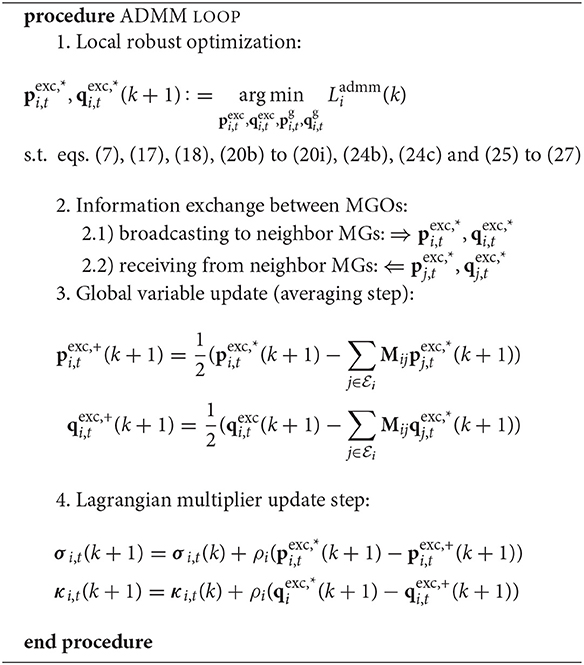
Algorithm 1 ADMM for robust networked-MG scheduling.

The algorithm comprises the local maximization step, global variable update and Lagrangian multiplier update. As shown in the algorithm, the local maximization step solves the local version of the revenue maximization problem while the consensus constraints eqs. (17) and (18) are taken into account in the augmented Lagrangian. The global variable update requires the communication between interconnected neighboring MGs. Note that the consensus constraints are only defined for active/reactive power in this work. The voltage magnitude of the coupled nodes is implicitly updated from one MG to another, i.e., after obtaining the voltage magnitude as per the local maximization step in one MG, the rest of the MGs are updated with the result and use it as the reference node voltage. Since the constraints are linear in a problem eq. (20) with a quadratic objective, the problem is hence a convex optimization problem. The convergence of solving convex optimization problems using the ADMM algorithm is proved in Boyd et al. (2011). In addition, upon the convergence of the ADMM, the solution converges to KKT stationary points (Erseghe, 2014, Theorem 1) (i.e., local minimum for non-convex scenarios and global minimum for convex scenarios). Having solved problem eq. (28). with ADMM, we use the following scheme to clear the market providing the optimality guarantee. For the local MG cost optimization problem eq. (28), the energy exchange price vectors α_i, β_i can be determined uniquely by σ_i and κ_i, i.e.,

$\begin{array}{ll}{\alpha }_i={\sigma }_i,{\beta }_i={\kappa }_i.& (30)\end{array}$

such that the optimality conditions of the overall system described by eq. (28) corresponds to the market equilibrium, where each MG optimizes their revenue based on the price setting eq. (30). From a practical perspective, the proposed adoption of the ADMM-structured method relies on solving the exchange problem in a decentralized manner with P2P communication between the MGOs. In practice, the first two steps in the ADMM loop can take place in either order without affecting the convergence. This kind of asynchronous update may provide benefits in dealing with communication delays and packet loss (see the exposition by Xu et al., 2019). Moreover, the choice of penalty factor ρ will significantly influence the convergence rate as well (Boyd et al., 2011), where different adaptive strategies are of interest to pre-condition and change ρ in an effective manner (see, e.g., Xu et al., 2017).

4.2. Optimal Exchange Price Decomposition

Consider the robust optimization problem of MGs i in eq. (28). The associated Lagrangian of the local optimization problem is:

$\begin{array}{l}{L}_i={\displaystyle \sum _{t=1}^T(}{\alpha }_{i,t}^{⊺}{p}_{i,t}^{\text{exc}}+{\beta }_{i,t}^{⊺}{q}_{i,t}^{\text{exc}}+{\displaystyle \sum _{\text{x}\in \{\text{g},\text{fl},\text{b}\}}{C}_t^{\text{x}}}(p_t^{\text{x}})+({\mu }_{i,t}^{\text{p,prox}}\\ +{\gamma }_{i,t}^{\text{mean}}·p_{i,t}^{\text{pcc}}))+{\Gamma }^{\text{p}}·{\mu }_i^{\text{p,sum}}+{\displaystyle \sum _{t=1}^T(}{\text{λ}}_{i,t}^{\text{p}}(p_{i,t}^{⊺}{1}_{n_i+1})\\ +{\text{λ}}_{i,t}^{\text{q}}(q_{i,t}^{⊺}{1}_{n_i+1})+({\overline{\mu }}_i^{\text{p}}{)}^{⊺}(p_{i,t}^{\text{g}}-{\overline{p}}_{i,t}^{\text{g}})-({\underset{\_}{\mu }}_i^{\text{p}}{)}^{⊺}(p_{i,t}^{\text{g}}-{\underset{\_}{p}}_{i,t}^{\text{g}})\\ +({\overline{\mu }}_i^{\text{fl}}{)}^{⊺}(p_{i,t}^{\text{fl}}-{\overline{p}}_{i,t}^{\text{fl}})-({\underset{\_}{\mu }}_i^{\text{fl}}{)}^{⊺}(p_{i,t}^{\text{fl}}-{\underset{\_}{p}}_{i,t}^{\text{fl}})\\ +({\overline{\mu }}_i^{\text{q}}{)}^{⊺}(q_{i,t}^{\text{g}}-{\overline{q}}_{i,t}^{\text{g}})-({\underset{\_}{\mu }}_i^{\text{q}}{)}^{⊺}(q_i^{\text{g}}-{\underset{\_}{q}}_i^{\text{g}})\\ +({\overline{\mu }}_i^{\text{l}}{)}^{⊺}(\left|Y_i^{\text{line}}\right|(C_i^{\text{f}}-C_i^{\text{t}})v_{i,t}-\left|{\overline{l}}_i\right|)-({\underset{\_}{\mu }}_i^{\text{l}}{)}^{⊺}(|Y_i^{\text{line}}|\\ (C_i^{\text{f}}-C_i^{\text{t}})v_{i,t}+\left|{\overline{l}}_i\right|)+({\overline{\mu }}_i^{\text{v}}{)}^{⊺}(v_{i,t}-{\overline{v}}_i)\\ -({\underset{\_}{\mu }}_i^{\text{v}}{)}^{⊺}(v_i-{\underset{\_}{v}}_i)+({\lambda }_{i,t}^{\text{bess}}{)}^{⊺}(so{c}_{i,t}-so{c}_{i,0}\\ +{\text{diag}}^{-1}(Q_{i,t}){\displaystyle \sum _{k=1}^t(\frac{1}{{\eta }^d}{p}_{i,k}^{\text{d}}-{\eta }^c{p}_{i,k}^{\text{c}})}\Delta t)).\end{array}$

The Karush-Kuhn-Tucker (KKT) conditions for the local optimization problem comprises the following first-order optimality condition on variable ${\text{p}}_i^{\mathrm{\text{exc}}}$:

$\begin{array}{l}\frac{\partial L_i}{\partial {\text{p}}_{i,t}^{\text{exc}}}:={\alpha }_i+{\left({\text{A}}_{i,t}^{\text{exc}}\right)}^{⊺}({\text{λ}}_i^{\text{p}}{1}_{n_i})\\ +{(\frac{\partial {\text{v}}_{i,t}}{\partial {\text{p}}_{i,t}^{\text{exc}}})}^{⊺}({\overline{\mu }}_i^{\text{v}}-{\underset{\_}{\mu }}_i^{\text{v}})+{(\frac{\partial {\text{v}}_{i,t}}{\partial {\text{p}}_{i,t}^{\text{exc}}})}^{⊺}{\left({\text{C}}_i^{\text{f}}-{\text{C}}_i^{\text{t}}\right)}^{⊺}|{\text{Y}}_i^{\text{line}}{|}^{⊺}\\ ({\overline{\mu }}_i^{\text{l}}-{\underset{\_}{\mu }}_i^{\text{l}})=0& (31)\end{array}$

together with primal/dual feasibility and complementary slackness (Boyd and Vandenberghe, 2004). We obtain

$\begin{array}{l}{\alpha }_i=-({({\text{A}}_{i,t}^{\text{exc}})}^{⊺}({\text{λ}}_i^{\text{p}}{1}_{n_i})+(\frac{\partial {\text{v}}_{i,t}}{\partial {\text{p}}_{i,t}^{\text{exc}}}{)}^{⊺}({\overline{\mu }}_i^{\text{v}}-{\underset{\_}{\mu }}_i^{\text{v}})\\ +(\frac{\partial {\text{v}}_{i,t}}{\partial {\text{p}}_{i,t}^{\text{exc}}}{)}^{⊺}({\text{C}}_i^{\text{f}}-{\text{C}}_i^{\text{t}}{)}^{⊺}|{\text{Y}}_i^{\text{line}}{|}^{⊺}({\overline{\mu }}_i^{\text{l}}-{\underset{\_}{\mu }}_i^{\text{l}}))& (32)\end{array}$

The results make intuitive sense: The price is decomposed into three parts: energy, voltage, and congestion as in the locational marginal prices formulation (see, e.g., Zhang et al., 2020).

5. Simulation Setup and Results

We tested the proposed ancillary service market framework on a 144-node AC distribution grid (Khodr et al., 2008), which was partitioned into three autonomous MGs. The topology of the test network is illustrated in Figure 5. Each MGO operated a number of DGs locally. One coupled node (node 7) was the energy exchange node, which connected MGs 1, 2, and 3. The test network had a total fixed nominal load of 11.9 MW and 7.38 Mvar. The cost coefficient for the DGs and BESSs are presented in Table 1. The uncertain price and load profile is depicted in Figure 6, where an ARMA model is used to generate 1,000 scenarios for prices and loads based on historical data taken from the Nation Singapore Electricity Market EMCS from year 2014 to 2015. The upper and lower bounds for the uncertain quantities were determined as the 95% confidence interval for the reduced scenarios. For the sake of simplicity, same load shape was applied to all MGs. Voltage constraints were kept as [0.95, 1.05]; the ADMM parameters were set as: η = 0.1, τ = 0.1, κ = 10, ${\rho }_i(0)=1.0\times 10^3,{\text{λ}}_i(0)=0,i\in \mathcal{M}\mathcal{G}$. The simulations were performed on a personal computer with Intel i7-8665U 3.2 Ghz and 24 GB RAM. The validation of the proposed framework was separated into the robust optimization part and the distributed optimization part.

FIGURE 5

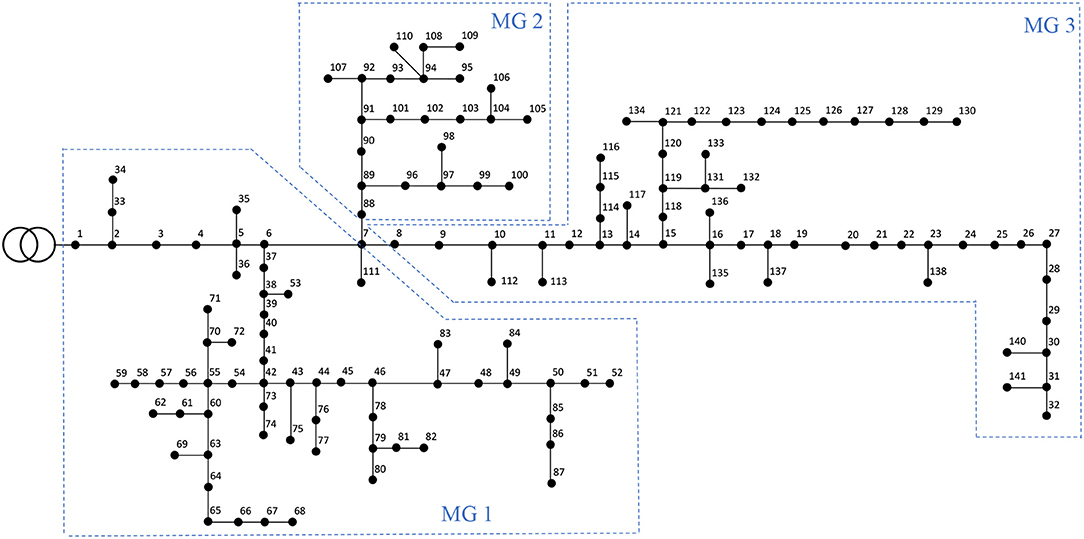
Figure 5. Simplified schematic of the 144-node test case (Khodr et al., 2008) partitioned into three autonomous MGs.

TABLE 1

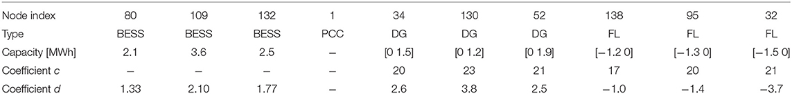
Table 1. Distributed generators (DG)/FL cost.

FIGURE 6

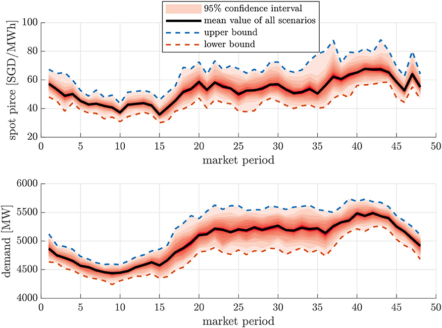
Figure 6. ARMA model for price and load profile based on data from EMC Singapore.

5.1. Case Study of Robust Optimization

In the case study, each DG has a limited generation capacity such that the collective supply from all DGs cannot meet the total demand from all nodes. Therefore, the PCC that connects to MG 1 provides energy to meet the energy demand for all MGs. The first part of the case study is to investigate the robust optimization for the networked MGs, where the performance under different parameter settings for Γ^D ∈ [0 1] and Γ^p ∈ [0 48] are tested. To show the impact of conservatism Γ^p, the worst-case realization of the wholesale market electricity price are obtained for different values of Γ^p, which is depicted in Figure 7. With the increasing value of conservatism, the worst-case scenarios for the prices tend to locate at the upper bound of the uncertain price. The most conservative decision (Γ^p = 48) to schedule the energy consumption, however, does not corresponds to the upper bound of the energy prices. This is due to the charge and discharge costs that occurs when using the battery to shift the energy consumption from the peak-price area to the low-price area. More specifically, to charge/discharge the battery at a higher power rate may result in a higher cost for the battery aging that makes this options less cost effective for obtaining the optimal energy dispatch schedule. On the other side, one can observe that the worst-case realization of the uncertain prices can only have deviations in the upper halves of the uncertain intervals. To show the impact of parameter settings for Γ^D, the results for different parameter settings Γ^D are presented in Figure 8. The worst-case scenario for the load profile realization is located at the upper bound, where the conservatism is set at its maximum.

FIGURE 7

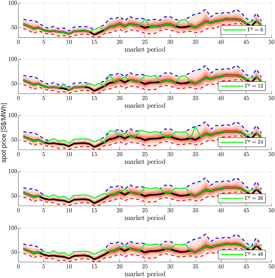
Figure 7. Worst-case scenario realization of power common coupling (PCC) price under different conservatism parameters Γ^p (Γ^D = 1).

FIGURE 8

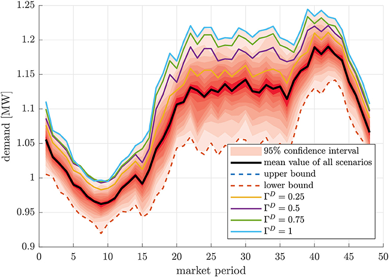
Figure 8. Worst-case scenario realization of uncertain load under different Γ^D (Γ^p = 8).

In practice, the parameter for conservatism should be predefined by the MGOs before solving the robust multiple-MG energy exchange scheduling problem. The actual cost for each MGO is dependent on the relative error of the worst-case scenario solution for the given degree of conservatism to the actual realization of the uncertain price. This can be shown by calculating the average relative error between the generated worst-case scenario value of the uncertain price from the robust optimization ${\gamma }_t^{robust}$ and its actual realization ${\gamma }_t^{actual}$, denoted as ϵ, i.e.,

$\begin{array}{ll}ϵ=\frac{1}{T}{\displaystyle \sum _{t\in \mathcal{T}}}|\frac{{\gamma }_t^{actual}-{\gamma }_t^{robust}}{{\gamma }_t^{actual}}|.& (33)\end{array}$

We plot the actual networked MG system operational cost compared to the relative error in Figure 9. The actual total cost is calculated based on actual energy prices and the pre-scheduled energy consumption. It can be observed that the most-conservative decision for the energy price does not necessarily lead to the most costly energy dispatch schedule. A higher conservatism parameter value ensures better solution robustness, which does not necessarily increase the cost. Furthermore, a direct correlation between the relative error of the robust prices and the actual prices can be obtained for different conservatism parameter settings. Therefore, a well-chosen parameter for the conservatism setting should well represent the probability that such a worst-case scenario occurs while maintaining the robustness of the solution.

FIGURE 9

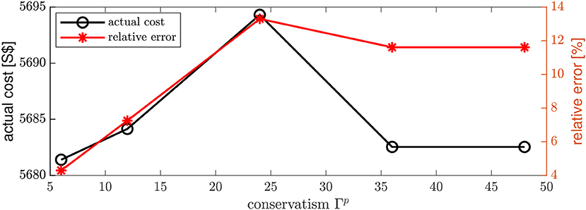
Figure 9. Correlation between the relative error of the robust schedule and energy cost.

5.2. Validation of Distributed Solution

To validate the distributed solution, we solve the robust networked MG exchange problem both in a centralized fashion and distributed fashion based on proposed method. The SOCs results of the BESSs are first presented in Figure 10A for ADMM and centralized solution, respectively. Since the battery aging cost for BESS 3 is the lowest, it can be observed that BESS 3 is utilized at its full capacity to provide energy balance. All three BESSs are discharged when the spot price at the PCC and the total demand is high. One can also conclude from Figure 10A that the centralized solution fully coincides with the distributed solution.

FIGURE 10

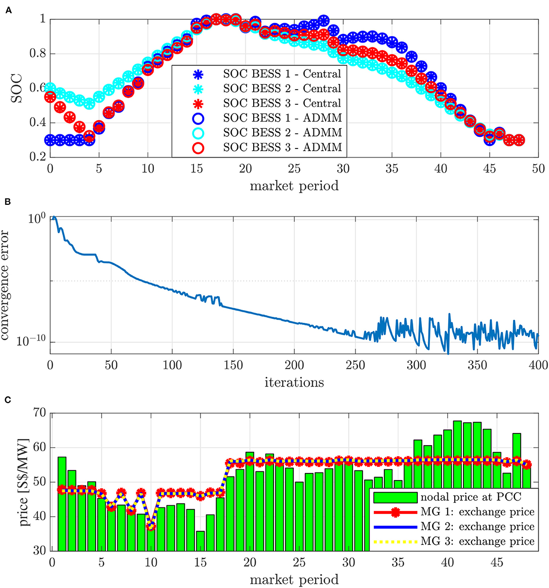
Figure 10. (A) SOC schedule for both the centralized method and ADMM; (B) ADMM convergence on primal residual; (C) energy exchange price (Γ^p = 8, Γ^D = 0.5).

The convergence of the distributed solution is shown in Figure 10B, where the convergence indicator of the ADMM is given as the primal residual r(k), i.e.,

$\begin{array}{ll}r(k)={\displaystyle \sum _{i\in \mathcal{M}}}{\displaystyle \sum _{t\in \mathcal{T}}}\left({\text{p}}_{i,t}^{\text{exc}}(k)-{\text{p}}_{i,t}^{\text{exc,+}}(k)+{\text{q}}_{i,t}^{\text{exc}}(k)-{\text{q}}_{i,t}^{\text{exc,+}}(k)\right).& (34)\end{array}$

In this part of the case study, the energy exchanged between all three MGs is also supplied by the PCC, where the baseline energy exchange prices are determined by PCC spot prices. The market-clearing price for the energy exchange between the MGs upon convergence of the ADMM is shown in Figure 10C, where the electricity price at the PCC provides the baseline price for the electricity exchange. Since the BESS is utilized to behave as a price arbitrager, the exchange price is flattened. It can also be observed that consensus is reached for the energy import/export on the coupled bus. Due to the existence of BESS as a price arbitrageur in balancing the energy supply and demand, the energy exchange price between multiple MGs are flattened compared to the spot price at the PCC.

The validation is further extended under binding thermal constraints for line flows, where additional constraints are added to the line current magnitude in MG 3. Consequently, MG 3 is fully supplied by its local DG generation with a higher marginal cost. We plot the electricity exchange schedule in Figure 11B, where zero electricity import for MG 3 can be observed. Compared to the non-congested scenario, the market-clearing price for energy exchange is increased as shown in Figure 11A. This is because the MGs have to pay the congestion part in the exchange price in addition to the baseline price as discussed in eq. (32).

FIGURE 11

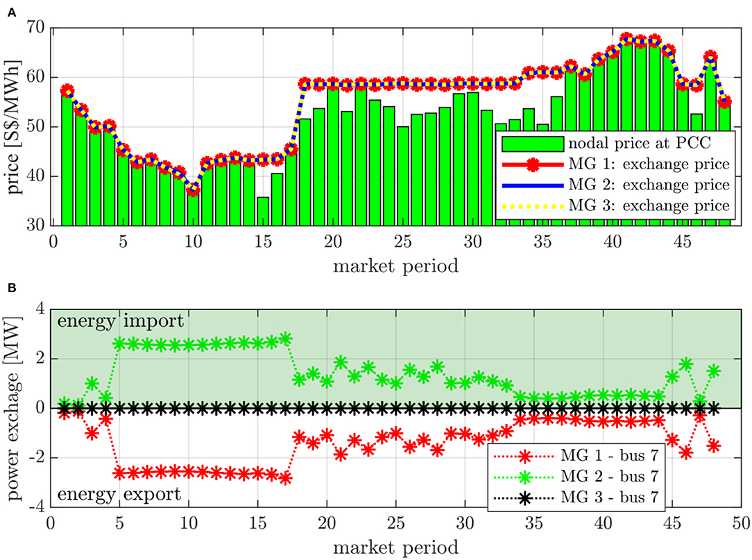
Figure 11. Congested test scenario: (A) energy exchange price; (B) energy exchange schedule between MGs (Γ^p = 8, Γ^D = 0.5).

6. Conclusion and Outlook

Moving toward the grid decentralization, a market framework for clearing the energy trading in the networked MG system is proposed in this work. The proposed ADMM-structured robust optimization method allows the robust scheduling for energy dispatch for DERs and MGs considering uncertain electricity prices, load, and DG generation variations while each local MG operation preserves its autonomy in the energy trading to achieve the optimality of the overall system. The numerical analysis provides insights for price settling when applying such a framework to different scenarios (cases). Note that from the market design perspective, we assume that each MGO is a price-taker without modeling their strategic behavior. In cases with a limited number of market participants (e.g., only two geographically connected microgrids), market power can be easily exercised, whereby an ADMM-based market mechanism cannot guarantee social-welfare optimality. Therefore, game-theoretical approaches are more appropriate for solving the energy exchange problem and providing the market design for these cases. Another interesting direction is to investigate the co-optimization of reserve provision of the networked MG system, which is considered as one of the future extensions for this proposal.

Data Availability Statement

The raw data supporting the conclusions of this article will be made available by the authors, without undue reservation.

Author Contributions

KZ designed the methodologies and performed the simulation. ST contributed to the literature analysis and provided a critical review. Both KZ and ST wrote the paper.

Funding

This work was supported by the Singapore National Research Foundation under its Campus for Research Excellence and Technological Enterprise Programme.

Conflict of Interest

The authors declare that the research was conducted in the absence of any commercial or financial relationships that could be construed as a potential conflict of interest.

References

Alam, M. N., Chakrabarti, S., and Ghosh, A. (2019). Networked microgrids: state-of-the-art and future perspectives. IEEE Trans. Ind. Inform. 15, 1238–1250. doi: 10.1109/TII.2018.2881540

CrossRef Full Text | Google Scholar

Bazmohammadi, N., Tahsiri, A., Anvari-Moghaddam, A., and Guerrero, J. M. (2019a). A hierarchical energy management strategy for interconnected microgrids considering uncertainty. Int. J. Electric. Power Energy Syst. 109, 597–608. doi: 10.1016/j.ijepes.2019.02.033

CrossRef Full Text | Google Scholar

Bazmohammadi, N., Tahsiri, A., Anvari-Moghaddam, A., and Guerrero, J. M. (2019b). Stochastic predictive control of multi-microgrid systems. IEEE Trans. Ind. Appl. 55, 5311–5319. doi: 10.1109/TIA.2019.2918051

CrossRef Full Text | Google Scholar

Bazmohammadi, N., Tahsiri, A., Tahsiri, A., Anvari-Moghaddam, A., and Guerrero, J. M. (2018). Optimal operation management of a regional network of microgrids based on chance-constrained model predictive control. IET Gen. Transm. Distrib. 12, 3772–3779. doi: 10.1049/iet-gtd.2017.2061

CrossRef Full Text | Google Scholar

Bolognani, S., and Dörfler, F. (2015). “Fast power system analysis via implicit linearization of the power flow manifold,” in 2015 53rd Annual Allerton Conference on Communication, Control, and Computing (Allerton, IL), 402–409. doi: 10.1109/ALLERTON.2015.7447032

CrossRef Full Text | Google Scholar

Boyd, S., Parikh, N., Chu, E., Peleato, B., and Eckstein, J. (2011). Distributed optimization and statistical learning via the alternating direction method of multipliers. Foundat. Trends Mach. Learn. 3, 1–122. doi: 10.1561/2200000016

CrossRef Full Text | Google Scholar

Boyd, S., and Vandenberghe, L. (2004). Convex Optimization. New York, NY: Cambridge University Press.

Google Scholar

Correa-Florez, C. A., Michiorri, A., and Kariniotakis, G. (2020). Optimal participation of residential aggregators in energy and local flexibility markets. IEEE Trans. Smart Grid 11, 1644–1656. doi: 10.1109/TSG.2019.2941687

CrossRef Full Text | Google Scholar

Cuffe, P., Smith, P., and Keane, A. (2014). Capability chart for distributed reactive power resources. IEEE Trans. Power Syst. 29, 15–22. doi: 10.1109/TPWRS.2013.2279478

CrossRef Full Text | Google Scholar

Daneshvar, M., Mohammadi-Ivatloo, B., Asadi, S., Anvari-Moghaddam, A., Rasouli, M., Abapour, M., et al. (2020a). Chance-constrained models for transactive energy management of interconnected microgrid clusters. J. Clean. Prod. 271:122177. doi: 10.1016/j.jclepro.2020.122177

CrossRef Full Text | Google Scholar

Daneshvar, M., Mohammadi-ivatloo, B., Zare, K., Asadi, S., and Anvari-Moghaddam, A. (2020b). A novel operational model for interconnected microgrids participation in transactive energy market: a hybrid IGDT/stochastic approach. IEEE Trans. Ind. Inform. 17, 4025–4035. doi: 10.1109/TII.2020.3012446

CrossRef Full Text | Google Scholar

Erseghe, T. (2014). Distributed optimal power flow using ADMM. IEEE Trans. Power Syst. 2015, 2370–2380. doi: 10.1109/TPWRS.2014.2306495

CrossRef Full Text | Google Scholar

Farivar, M., Chen, L., and Low, S. (2013). “Equilibrium and dynamics of local voltage control in distribution systems,” in 52nd IEEE Conference on Decision and Control (Florence), 4329–4334. doi: 10.1109/CDC.2013.6760555

CrossRef Full Text | Google Scholar

González, M., Miguel, J., Conejo, A. J., Madsen, H., Pinson, P., and Zugno, M. (2014). Integrating Renewables in Electricity Markets: Operational Problems. Springer. doi: 10.1007/978-1-4614-9411-9

CrossRef Full Text | Google Scholar

Guerrero, J. M., Chandorkar, M., Lee, T. L., and Loh, P. C. (2013). Advanced control architectures for intelligent microgrids; part I: decentralized and hierarchical control. IEEE Trans. Ind. Electron. 60, 1254–1262. doi: 10.1109/TIE.2012.2194969

CrossRef Full Text | Google Scholar

Hanif, S., Gooi, H. B., Massier, T., Hamacher, T., and Reindl, T. (2017). Distributed congestion management of distribution grids under robust flexible buildings operations. IEEE Trans. Power Syst. 32, 4600–4613. doi: 10.1109/TPWRS.2017.2660065

CrossRef Full Text | Google Scholar

Hirsch, A., Parag, Y., and Guerrero, J. (2018). Microgrids: a review of technologies, key drivers, and outstanding issues. Renew. Sustain. Energy Rev. 90, 402–411. doi: 10.1016/j.rser.2018.03.040

CrossRef Full Text | Google Scholar

Huang, R., Huang, T., Gadh, R., and Li, N. (2012). “Solar generation prediction using the ARMA model in a laboratory-level micro-grid,” in 2012 IEEE Third International Conference on Smart Grid Communications (SmartGridComm) (Tainan), 528–533. doi: 10.1109/SmartGridComm.2012.6486039

CrossRef Full Text | Google Scholar

Khodr, H., Olsina, F., Jesus, P. D. O. D., and Yusta, J. (2008). Maximum savings approach for location and sizing of capacitors in distribution systems. Electric Power Syst. Res. 78, 1192–1203. doi: 10.1016/j.epsr.2007.10.002

CrossRef Full Text | Google Scholar

Kim, T. T., and Poor, H. V. (2011). Scheduling power consumption with price uncertainty. IEEE Trans. Smart Grid 2, 519–527. doi: 10.1109/TSG.2011.2159279

CrossRef Full Text | Google Scholar

Liu, Y., Gooi, H. B., and Xin, H. (2017). “Distributed energy management for the multi-microgrid system based on ADMM,” in 2017 IEEE Power Energy Society General Meeting (Chicago, IL), 1–5. doi: 10.1109/PESGM.2017.8274099

CrossRef Full Text | Google Scholar

Liu, Z., Wang, L., and Ma, L. (2020). A transactive energy framework for coordinated energy management of networked microgrids with distributionally robust optimization. IEEE Trans. Power Syst. 35, 395–404. doi: 10.1109/TPWRS.2019.2933180

CrossRef Full Text | Google Scholar

Ma, W., Wang, J., Gupta, V., and Chen, C. (2018). Distributed energy management for networked microgrids using online admm with regret. IEEE Trans. Smart Grid 9, 847–856. doi: 10.1109/TSG.2016.2569604

CrossRef Full Text | Google Scholar

Rahimi, F., Ipakchi, A., and Fletcher, F. (2016). The changing electrical landscape: end-to-end power system operation under the transactive energy paradigm. IEEE Power Energy Mag. 14, 52–62. doi: 10.1109/MPE.2016.2524966

CrossRef Full Text | Google Scholar

Sabounchi, M., and Wei, J. (2017). “Towards resilient networked microgrids: blockchain-enabled peer-to-peer electricity trading mechanism,” in 2017 IEEE Conference on Energy Internet and Energy System Integration (EI2) (Beijing), 1–5. doi: 10.1109/EI2.2017.8245449

CrossRef Full Text | Google Scholar

Saraiva, J. T., and Gomes, M. H. (2010). “Provision of some ancillary services by microgrid agents,” in 2010 7th International Conference on the European Energy Market (Madrid), 1–8. doi: 10.1109/EEM.2010.5558756

CrossRef Full Text | Google Scholar

Shahidehpour, M., Li, Z., Bahramirad, S., Li, Z., and Tian, W. (2017). Networked microgrids: exploring the possibilities of the IIT-Bronzeville grid. IEEE Power Energy Mag. 15, 63–71. doi: 10.1109/MPE.2017.2688599

CrossRef Full Text | Google Scholar

Trpovski, A., Recalde, D., and Hamacher, T. (2018). “Synthetic distribution grid generation using power system planning: case study of Singapore,” in 2018 53rd International Universities Power Engineering Conference (UPEC) (Glasgow, UK), 1–6. doi: 10.1109/UPEC.2018.8542054

CrossRef Full Text | Google Scholar

Wang, R., Wang, P., and Xiao, G. (2015). A robust optimization approach for energy generation scheduling in microgrids. Energy Convers. Manage. 106, 597–607. doi: 10.1016/j.enconman.2015.09.066

CrossRef Full Text | Google Scholar

Wang, Z., Chen, B., Wang, J., Begovic, M. M., and Chen, C. (2015). Coordinated energy management of networked microgrids in distribution systems. IEEE Trans. Smart Grid 6, 45–53. doi: 10.1109/TSG.2014.2329846

CrossRef Full Text | Google Scholar

Weron, R. (2005). Heavy Tails and Electricity Prices. HSC Research Reports HSC/05/02, Hugo Steinhaus Center, Wroclaw University of Technology.

Google Scholar

Wu, Y., Barati, M., and Lim, G. (2019). A pool strategy of microgrid in power distribution electricity market. IEEE Trans. Power Syst. 35, 3–12. doi: 10.1109/TPWRS.2019.2916144

CrossRef Full Text | Google Scholar

Xu, J., Sun, H., and Dent, C. J. (2019). Admm-based distributed opf problem meets stochastic communication delay. IEEE Trans. Smart Grid 10, 5046–5056. doi: 10.1109/TSG.2018.2873650

CrossRef Full Text | Google Scholar

Xu, Z., Figueiredo, M., and Goldstein, T. (2017). “Adaptive ADMM with spectral penalty parameter selection,” in Proceedings of the 20th International Conference on Artificial Intelligence and Statistics, Volume 54 of Proceedings of Machine Learning Research, eds A. Singh and J. Zhu (Fort Lauderdale, FL: PMLR), 718–727.

Google Scholar

Zhang, K., Troitzsch, S., Hanif, S., and Hamacher, T. (2020). Coordinated market design for peer-to-peer energy trade and ancillary services in distribution grids. IEEE Trans. Smart Grid 11, 2929–2941. doi: 10.1109/TSG.2020.2966216

CrossRef Full Text | Google Scholar

Zimmerman, R. D., and Murillo-Śanchez, C. E. (2020). Matpower User's Manual, Version 7.1. doi: 10.5281/zenodo.4074122

CrossRef Full Text | Google Scholar