Accurate and Rapid Forecasts for Geologic Carbon Storage via Learning-Based Inversion-Free Prediction

1 Introduction

Carbon capture and storage (CCS) has been proposed as a strategy to reduce greenhouse gas emissions entering the atmosphere from stationary sources and thereby help to mitigate the global climate crisis (Pacala and Socolow, 2004; Alcalde et al., 2018). For example, the Intergovernmental Panel on Climate Change (IPCC) estimated that capturing CO₂ at a modern conventional power plant could reduce CO₂ emissions to the atmosphere by approximately 80–90% compared to a plant that does not have the technology to capture carbon (IPCC report, Metz et al. (2005)). Once the CO₂ has been captured, it must be permanently stored and isolated from the atmosphere, and carbon storage in geological formations is a proven method to store CO₂ at significant (commercial) scales, e.g., one million metric tons per year or greater. The U.S. Department of Energy’s (DOE) National Energy Technology Laboratory (NETL) has been working with Regional Carbon Sequestration Partnerships through the Carbon Storage Program to identify prospective sites within the United States for the geologic storage of CO₂ (DOE-NETL about the carbon storage program, 2021). Since 2007, NETL has published several assessments of CO₂ storage resource potential in geologic formations and terrestrial sinks in the United States, considering the following geologic formations as viable targets for CO₂ storage: saline formations, coal seams, conventional hydrocarbon reservoirs, basalt formations, and unconventional oil and gas formations including shales and tight sands (DOE-NETL carbon storage Atlas, 2015).

The present work focuses on storage in saline reservoirs, which provide significantly larger storage capacity, are globally more ubiquitous (Ji and Zhu, 2015) and have few competing uses than hydrocarbon reservoirs. Although depleted oil and gas reservoirs may provide important intermediate-scale storage, any CCS-activity, at a scale sufficient to impact the carbon problem (e.g., billions of metric tons), will necessarily involve large-scale CO₂ injections into deep saline aquifers (e.g., multiple projects inject one million metric tons per year or greater). However, CCS projects generally target “green field sites,” where there is often little characterization data and therefore large uncertainty about the petrophysical properties and other geologic attributes of the storage reservoir (Brandt et al., 2014; Celia et al., 2015). Uncertainty associated with predicting subsurface response to CO₂ injection is a key challenge to project developers seeking to secure financing, permits, and social license to inject CO₂ into the storage reservoir (Namhata et al., 2016; Chen et al., 2020). Due to the inherent uncertainty about the storage reservoir, ensemble-based approaches are often used to forecast multiple realizations prior to CO₂ injection to visualize a range of potential outcomes. In addition, monitoring data during injection operations are used to update the pre-injection forecasts and thereby improve agreement between forecasted and observed behavior. Today, forecasting the subsurface response to CO₂ injection requires detailed three-dimensional (3D) geologic models coupled with numerical reservoir simulation, which are labor- and time-intensive and require specialists with backgrounds in petrophysics, geology, and reservoir engineering. Providing CO₂ storage site operators and regulators with rapid forecasting tools for timely decision making is essential to addressing these challenges to CCS project development and management. Delivering on this need requires transformational changes in how we predict subsurface responses to CO₂ injection and update those predictions using monitoring measurements.

Different methods have been employed to forecast geological carbon storage scenarios including analytical solutions and numerical simulations. Analytical methods are useful in providing quick evaluations with minimum input data and they are free from numerical artifacts (Celia et al., 2005; Guo et al., 2014; Qiao et al., 2021). Numerical simulations, on the other hand, have been widely used in large-scale projects (Pawar et al., 2009; Humez et al., 2011). However, numerical approaches (e.g., compositional reservoir simulation) usually require significant computational time and detailed geological data and measurements that may not always be available. In this study, we use machine learning techniques to address some of the challenges of numerical methods.

The conventional numerical method for predicting CO₂ distribution in a reservoir relies heavily on inverse modeling (history matching, calibration) to constrain uncertain parameters in complex reservoir simulation models (Bianco et al., 2007; Oliver and Chen, 2011; Doughty and Oldenburg, 2020). This inversion-based prediction approach has limitations for rapid integration of observation data and providing timely decision support due to the following reasons: 1) Model inversion is computationally expensive and can require tens of thousands of expensive reservoir model simulations. Not all these simulations can be conducted concurrently and thus cannot take full advantage of contemporary parallel computing resources (each forward simulation may be parallelizable and a set of forward simulations may be conducted concurrently, but most inverse methods are essentially iterative and cannot achieve full parallelism). 2) Model inversion can be numerically ill-posed resulting in poor predictions when the number of parameters is greater than the number of independent observations, which is usually the case in geological carbon storage simulation. 3) Model inversion needs to be repeated when incorporating new observations. 4) Reservoir simulation models are based on geologic models, which may artificially constrain simulations and are slow and expensive to update with new field (as opposed to operational) data.

To address these challenges, our research aims to develop machine learning (ML) techniques with a potential to provide significant improvements to the conventional history matching-based forecasts, thus enhancing the timeliness and accuracy of information provided to the operator. This paper describes our methods and analyzes their performance in predicting the CO₂ plume and pressure distribution in the storage reservoir at a commercial-scale storage project. Our project is part of a large initiative called SMART (Science-informed Machine Learning for Accelerating Real Time Decisions in Subsurface Applications) funded by U.S. Department of Energy with the goal to enable better decisions in CO₂ storage operations.

2 Materials and Methods

We propose a Learning-based Inversion-free Prediction (LIP) framework that produces fast prediction with uncertainty quantification via integrating observations, based on parallel forward simulations. The observations can be streaming measurements that are obtained from point locations continuously or near-continuously in time such as pressure and CO₂ saturation data from a well, and they can also be a saturation distribution data from a time-lapse 3D seismic survey (4D seismic survey). In this study, we consider the former, the point data discrete in locations but continuous in time. The key idea of the LIP framework is to circumvent the challenge of inverse modeling by precomputing an ensemble of unconstrained forward simulations and then using ML methods to learn the relationship between simulated observation and prediction variables. Once the ML model has learned the relationship, it can be used to update the prediction of future system behavior from its prior distribution to the posterior distribution by integrating actual observed data. When additional observations are available, we retrain the ML model to update the observation-prediction relationship by extracting the corresponding simulated observation and prediction variable samples from the prior sample set. Because the ML model training is very fast (a few seconds by using LIP) and the incorporation of new observations does not require extra reservoir simulations (by extracting the simulated samples from the prior sample set), the LIP method enables rapid data assimilation and timely decision support. The new observations can be the transient data from the same location/well or can be the data from different locations or even different types of data. As long as these observation variables have been simulated in the forward model runs, there is no need in the LIP framework to perform additional forward simulations when incorporating the new observations.

The key of LIP is to establish an observation-prediction relationship from prior samples in a reduced dimension to be able to estimate posterior prediction distributions for given observations. Specifically, LIP consists of four steps:

1 Generating prior samples of observation and prediction variables by running forward models based on the prior distribution of model parameters;

2 Dimension reduction of the simulated observations and predictions;

3 Establishing a statistical relationship between observation and prediction in the reduced dimension;

4 Using Bayesian inference to calculate the posterior distribution of the prediction based on the statistical model and by integrating the observed data.

Steps 1-3 correspond to the training stage, where the observation-prediction relationship in the reduced dimension is learned from unconstrained forward simulations. Step 4 corresponds to the prediction stage, where the posterior distribution of the prediction is deduced from the observed data after back transformation to its original high-dimensional space. The LIP method can be generally applied to geological carbon storage problems. In this study, a clastic shelf model was considered as the geological model for a demonstration because the clastic shelf environment exhibits the greatest CO₂ storage rate in the model comparison study of Bosshart et al. (2018).

2.1 Model Description and Generation of Prior Samples

To meet the goal of producing results relevant to commercial-scale CCS operations and meanwhile being able to perform the model simulations in a reasonable time, a 3D model domain was designed at a resolution of 211 by 211 with 30 layers, i.e., 1,335,630 grid cells in total, where each cell has a size of 500 feet long, 500 feet wide, and 10 feet thick. The model has a flat structure and the storage formation is 4,000 feet deep. The model contains three facies: high-quality reservoir, low-quality reservoir, and cap rock. The top two layers of the model were assigned cap rock (shale) facies and they were given shale porosity and permeability values based upon previous work by Cavanagh and Wildgust (2011). In this study, we considered the uncertainty of porosity and permeability in the reservoir and generated their realizations in the following way.

All the realizations have the same rock facies geometry, but the porosity-permeability distributions differ. We sampled the porosity-permeability parameter space to generate the realizations. The Energy & Environmental Research Center at the University of North Dakota maintains an Average Global database (AGD) of paired porosity and permeability measurements for a host of lithologies, facies, and depositional environments (currently 26,700 + measurements) (Gorecki et al., 2009). The current work used a clastic shelf depositional environment and porosity-permeability paired samples specific to that environment. We first generated porosity realizations using Gaussian random function simulation with a variogram of 5,000 feet in the major and minor directions and 20 feet in the vertical direction. Permeability realizations were generated from the porosity-permeability cross-plots based on the derived relationship between these two variables from the AGD. We created 100 geological realizations (i.e., geomodels) using Schlumberger’s Petrel software suite that reflect the variation in porosity and permeability. The ensemble can be envisioned as a stratified sample, where the number of realizations is proportional to the probability distribution for porosity. For example, we sampled seven percentiles of p05, p10, p25, p50, p75, p90, and p95 to represent the low to high porosity/permeability and for each percentile we have the following number of realizations, 10, 15, 22, 23, 16, 9, and 5, respectively. Figure 1 shows the porosity and permeability fields of layer three for one realization from the p25, p50, and p75 geomodels. We can see that these geomodels have a large variation in porosity and permeability.

FIGURE 1

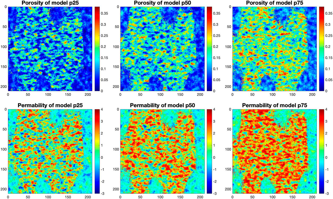
FIGURE 1. One realization of porosity (top) and permeability (bottom) fields of layer three for geomodels p25, p50, and p75. These three models have the same rock type geometry; the models p25, p50, and p75 correspond to low, mid, high porosity, respectively. The porosity color scale is a fraction from 0 to 0.4 (0–40% porosity) and the permeability color scale is the logarithm (base 10) of the permeability in millidarcys

For each geomodel, we performed a full equation-of-state compositional simulation (physics including convective and dispersive flow, residual gas trapping, CO₂ dissolution in aqueous phase, thermal capability) for 10 years using CMG-GEM (v2019), which is a reservoir simulator for compositional, chemical and unconventional reservoir modelling. The model was simulated using closed lateral and vertical boundaries. The temperature and pressure regimes for the simulation at 4000-foot depth were 120.778 4°F and 1,800.93 psi, respectively. The temperature and pressure were defined for each layer. They followed a linear pressure gradient of 0.43 psi/ft and a linear temperature gradient of 0.019 67°F/ft. Four injection wells—located regularly at the grid cells (71, 71, 3–30) (71, 141, 3–30), (141, 141, 3–30), and (141, 71, 3–30), respectively—inject CO₂ into the reservoir with a target mass injection rate of two million metric tons per year across all four wells. We simulated 10 years of injection with a 20 million metric tons CO₂ injection target (2 million metric tons per year × 10 years), to represent the earliest years of a commercial-scale storage project, during which CO₂ plumes are expected be the least predictable (i.e., the greatest rates of change per unit time). Maximum bottom hole pressure (BHP) constraint for each injector was Pf = 0.7 psi/ft. If BHP ≤ Pf, then CO₂ will continue to flow into the formation. However, if BHP $>$ Pf, then the injection rate for that well will slow down. We saved the simulation outputs of CO₂ plume and pressure distribution of the entire 3D domain at 32 time steps, i.e., monthly for years 1 and 2 and then annually for years 3–10. Each simulation takes about 7–10 h on average using 4–10 cores on an Intel Xeon Scalable (Cascade Lakes) CPU. The lengthy simulation time makes it really difficult, if not impossible, to enable conventional inversion-based history matching for timely forecasting.

In this study, we use the LIP method to predict the CO₂ plume and pressure distribution in layer 3 (the top model layer of the storage reservoir immediately below the cap rock layer) after 10 years of injection based on the saturation and pressure observations from the four injection wells in layer 3. For example, the prediction variables for pressure is the CO₂ pressure distribution at each of the 211 by 211 grid cells in layer 3 (44 ,521 variables in total) at year 10, and the observation variables are the four time-series of pressure-transients at the four wells in layer 3. We performed five case studies, depending on the duration of the observation period and thus the look-ahead period. We summarized the five cases in Table 1. Specifically, we forecasted pressure distribution in year 10 from the perspective of year 1, 2, 5, 7 and 9. In each case, we used only the data (both the simulated and observed data of observation variables) available up to that time, which corresponds to varying the look-ahead period from 9 years (i.e., the perspective of year 1 looking ahead to year 10) to 1 year (i.e., the perspective of year 9 looking ahead to year 10). For example, in Case I, we used 1 year of pressure-transient observations (12 time steps×4 wells = 48 observation variables) in layer three to predict the pressure distribution at each of the 211 by 211 grid cells in layer three at year 10; and in Case V, we used 9 years of observations (31 time steps×4 wells = 124 observation variables) to predict the pressure distribution in year 10. These five case studies were designed to evaluate LIP’s accuracy, efficiency, and capacity to incorporate streaming observations to improve prediction.

TABLE 1

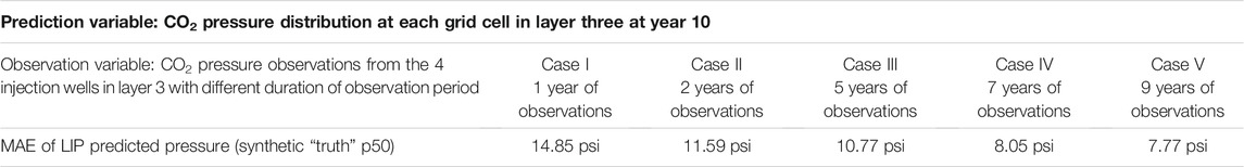
TABLE 1. Definition of the five case studies and the corresponding LIP method’s prediction performance. In the five cases, the prediction variables are the same which are the target we want to predict and the observation variables are different depending on the duration of the observation period. We investigate LIP’s predictive capability (measured by mean absolute error (MAE)) in incorporating different number of observation data.

These are challenging applications because of the large uncertain domain and the limited 100 geomodels and simulation samples. To evaluate LIP performance, we took one geomodel as a synthetic “truth” and used the other 99 geomodels to learn the observation-prediction relationship in above Steps 2–3. The corresponding pressure plume of the synthetic geomodel served as the reference against which we assessed our prediction results. To investigate the robustness of the LIP method for predicting the CO₂ plume and pressure field with different patterns, we made three choices of the synthetic geomodels corresponding to low, mid, and high porosity, i.e., picking one realization from the p25, p50, and p75 geomodels, respectively. For each synthetic case, we used the selected geomodel as reference and the other 99 geomodels for learning. In the similar manner to predict the pressure, we used the CO₂ saturation data in the four wells to predict the CO₂ plume in layer 3 after 10 years of injection. Figure 2 shows the 100 samples of the CO₂ pressure and saturation profile in the four wells over 10 years at the 32 time steps where we highlighted the three samples chosen as the synthetic observed data in the three synthetic cases (each dot in the highlighted line represents one time step). The figure indicates that the difference of the pressure and saturation among the samples is fairly large and our selected synthetic “truth” has a good representation of the low, mid, and high pressure/saturation. The small number of training data (99 geomodels) and the limited and non-smooth observation-transient data (monthly in first 2 years and annually in last 8 years) make the prediction problem rather challenging. In the following subsections of Section 2, we explain the key Steps 2-4 of the LIP method to solve this problem. In Section 3, we demonstrate how this problem was addressed using LIP.

FIGURE 2

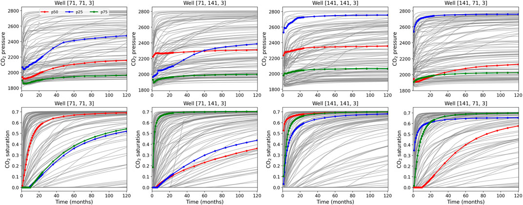
FIGURE 2. The 100 simulation outputs of CO₂ pressure and saturation profile in the four wells over 10 years at 32 time steps (identified by dots in the colored lines) where the first 24 time steps are monthly data and the last eight time steps are annual data. The highlighted three colored lines, which correspond to one realization of geomodels p25, p50, and p75 shown in Figure 1, were used as “synthetic” observed data.

2.2 Dimension Reduction

The prediction variable (denote as h) here is a spatial distribution and the observation variables (denote as d) are four time series, which have spatial and temporal correlations, respectively. When the variable dimensions are highly correlated with each other, multicollinearity occurs (Daoud, 2017). Multicollinearity results in numerical issues during model fitting and degrades predictive performance of the statistical model. One solution for addressing multicollinearity is dimension reduction. Dimension reduction identifies degrees of freedom that capture most of the variance in the data. Therefore, performing statistical analysis in the reduced dimension removes the multicollinearity and facilitates the model fitting. Additionally, dimension reduction reduces the number of variables and thus reduces the required number of samples, which improves the computational efficiency and enhances the model reliability.

We use principal component analysis (PCA) for dimension reduction. PCA is a multivariate analysis technique that applies an orthogonal transformation to convert a set of samples of possibly correlated variables into a set of values of uncorrelated variables, called principal components. Typically, the first a few components of the PCA decomposition explain most of the variance of the data. PCA is commonly used for dimensionality reduction by projecting each data point onto only the first few principal components to obtain lower-dimensional data while preserving as much of the data’s variation as possible. The first principal component can equivalently be defined as a direction that maximizes the variance of the projected data. The i^th principal component can be taken as a direction orthogonal to the first i − 1 principal component that maximizes the variance of the projected data.

Since our observation variables are from multiple sources (i.e., four injection wells), we use a mixed PCA to pool data together and generate a reduced dimensional projection of the combined data. First, a standard PCA is performed on each of the data source (i.e., the pressure transient from each injection well) to obtain the largest singular values. Next, each data source is normalized according to its first singular value; this accounts for any difference in scales amongst the data sources. Last, the normalized data inputs are concatenated and the standard PCA is applied to this final matrix. After dimension reduction, we obtain observation variables d^f and prediction variables h^f, respectively, in the reduced dimension. PCA is a bijective operation, so the original high-dimensional variable can be recovered uniquely by undoing the projection.

2.3 Establishing the Statistical Relationship

The relationship between d^f and h^f in the reduced dimension can be nonlinear which challenges the statistical model learning. We first use canonical correlation analysis (CCA) (Yang et al., 2021) to linearize the relationship and simplify the model fitting. CCA is a multivariate analysis method that can be applied to transform the relationships between pairs of vector variables into a set of independent linearized relationships between pairs of scalar variables. The resulting linear combinations are denoted as d^c and h^c, and called the canonical variates of d^f and h^f. The canonical transformation is found through the eigen-decomposition of the sample covariance matrix and this CCA transformation is reversible. If d^c and h^c in the canonical space are nearly linearly correlated, a linear model can be used to simulate their relationship. If after CCA, the relationship of d^c and h^c is still not quite linear, we can use advanced ML models such as neural networks for regression.

2.4 Bayesian Inference of the Prediction

We use Bayesian inference to estimate predictions. But unlike the traditional workflow which uses Bayesian methods to quantify uncertainties of model parameters first and then infer prediction uncertainties (Lu et al., 2017), we use Bayesian methods to calculate the posterior distribution of the predictions directly. Based on Bayes’ rule, the posterior distribution of a prediction variable h for some observed data d_obs is

$p\left(\mathbf{h}|{\mathbf{d}}_{obs}\right)\propto L\left(\mathbf{h}|{\mathbf{d}}_{obs}\right)p\left(\mathbf{h}\right),(1)$

where p(h) is the prior distribution and L (h|d_obs) is the likelihood function. PCA and CCA enable reducing a set of high-dimensional variables (d, h) to a set of low-dimensional and linearly correlated variables (d^c, h^c). We first estimate the posterior distribution $p({\mathbf{h}}^c|{\mathbf{d}}_{obs}^c)$ and then transform h^c back to its original space h. In the canonical space, $p({\mathbf{h}}^c|{\mathbf{d}}_{obs}^c)$ can be estimated by

$p\left({\mathbf{h}}^c|{\mathbf{d}}_{obs}^c\right)\propto L\left({\mathbf{h}}^c|{\mathbf{d}}_{obs}^c\right)p\left({\mathbf{h}}^c\right).(2)$

We use a linear model G to simulate the relationship between d^c and h^c, i.e., d^c = Gh^c. By assuming a Gaussian likelihood as commonly done in the CCS community (Oliver and Chen, 2011), $L({\mathbf{h}}^c|{\mathbf{d}}_{obs}^c)$ can be formulated as

$L\left({\mathbf{h}}^c|{\mathbf{d}}_{obs}^c\right)=\exp \left(-\frac{1}{2}{\left(G{\mathbf{h}}^c-{\mathbf{d}}_{obs}^c\right)}^T{\mathbf{C}}_{{\mathbf{d}}^c}^{-1}\left(G{\mathbf{h}}^c-{\mathbf{d}}_{obs}^c\right)\right).(3)$

where ${\mathbf{C}}_{{\mathbf{d}}^c}$ is the covariance matrix of the observation error. In this work, we are considering a synthetic case where the observed data is from one geomodel, so ${\mathbf{C}}_{{\mathbf{d}}^c}$ here is calculated as the covariance of the residuals from the linear model fitting.

Through normal score transformation based on the sample mean ${\bar{\mathbf{h}}}_{prior}^c$ and the sample covariance ${\mathbf{C}}_{{\mathbf{h}}^c}$ calculated from the prior samples of h^c, we obtain a Gaussian prior of h^c in the transformed space. Since the prior and the likelihood of h^c are both Gaussian, its posterior is also Gaussian and the posterior mean ${\tilde{\mathbf{h}}}^c$ and posterior covariance ${\tilde{\mathbf{C}}}_{{\mathbf{h}}^c}$ can be analytically estimated by

${\tilde{\mathbf{h}}}^c={\bar{\mathbf{h}}}_{prior}^c+{\mathbf{C}}_{{\mathbf{h}}^c}{G}^T{\left(G{\mathbf{C}}_{{\mathbf{h}}^c}{G}^T+{\mathbf{C}}_{{\mathbf{d}}^c}\right)}^{-1}\left({\mathbf{d}}_{obs}^c-G{\bar{\mathbf{h}}}_{prior}^c\right),(4)$

${\tilde{\mathbf{C}}}_{{\mathbf{h}}^c}={\left(G^T{\mathbf{C}}_{{\mathbf{d}}^c}^{-1}G+{\mathbf{C}}_{{\mathbf{h}}^c}^{-1}\right)}^{-1}.(5)$

An advantage of the Gaussian process regression is that a Gaussian distribution is uniquely defined by its mean and covariance and sampling a Gaussian distribution is straightforward. Then, based on Eqs 4, 5, we generate posterior samples of h^c directly. By undoing the normal score transformation followed by the back transformation of CCA, we obtain posterior samples of h^f. Next, after back transformation of PCA, we obtain the posterior samples of prediction quantity h in its original space. Based on these h samples, we then estimate posterior prediction distribution.

3 Results

In this section, we present the results of applying the LIP framework to the synthetic simulation cases to illustrate the LIP method and evaluate its prediction performance. We start with the most data-constrained case (Case V in Table 1) using 9 years of pressure transient data from the wells to predict the pressure distribution in year 10. Then, we discuss the results of additional cases (Case I – Case IV in Table 1) by incorporating 1, 2, 5, and 7 years of observations to assess the sensitivity of the LIP prediction performance to the available monitoring data and to evaluate the capability of LIP to incorporate additional observations for improving the prediction. Lastly, we show the results of applying the LIP framework to the CO₂ plume prediction.

In the following, we discuss the results using 9 years of pressure observations. We first use the synthetic case of p50 to demonstrate the LIP method, and then we analyze the prediction performance in detail for the three synthetic cases. In the LIP framework, after we generate the model simulation data from the geomodels, we perform the dimension reduction of the observation and prediction variables based on the simulation samples. Figure 3 shows the scree plots of the PCA (a line plot of cumulative variance versus number of principal components used to determine the number of principal components to keep in the PCA). We can see that the dimensions of both observation and prediction variables can be greatly reduced by keeping the first few components with a little information loss. Here, the observation variables are 9 years of pressure data from the four wells (i.e., 31 × 4 = 124 variables), and the prediction variables are the pressure distribution in each grid cell of layer three at year 10 (i.e., 211 × 211 = 44 ,521 variables). Figures 3A,B indicate that the first ten principal components capture 99% of variation in the observation variables d and that the first ten principal components capture 98% of variation in the prediction variables h. Based on these results from the dimension reduction step, for both variables we keep their first ten principal components and then establish the statistical relationship of d and h in their reduced ten dimensional space. Figures 3C, D, using one realization as a demonstration, indicate that keeping the first ten principal components we are able to recover the target pressure field with minor difference from its original pressure distribution where the mean absolute error is about 1.6 psi.

FIGURE 3

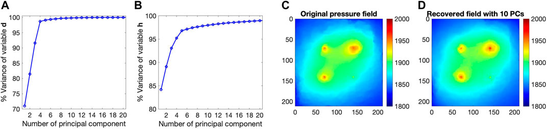
FIGURE 3. Scree plots of (A) observation variables d and (B) prediction variables h in PCA. (A) indicates that 10 principal components (PCs) can capture over 99% variation of the observation variable d; (B) shows that 10 PCs can capture about 98% variation of the prediction variable h. (C) CO₂ pressure field from the original data and (D) the recovered pressure field from inverse PCA using the preserved 10 PCs. The x- and y-axes for the pressure fields are the model x- and y-coordinates and the color map is pressure in psi from 1800 to 2000 psi.

Next, in the reduced observation-prediction dimensions, we perform the CCA for linear transformation. The scatter plot of Figure 4 indicates that after applying CCA, the canonical variates d^c and h^c have a strong linear correlation with coefficients of 0.99 and 0.92 for the first two principal components, respectively. The coefficients for the remaining eight principal components are also high, above 0.8 (results are not shown here). This suggests that a linear regression model can be established to simulate the relationship of d^c and h^c. In this study, both observation and prediction variables are the same type of quantity (i.e., CO₂ pressure) with smooth variation, so it is not very surprising that they show strong linear correlation here.

FIGURE 4

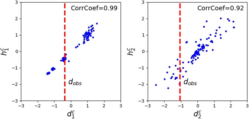
FIGURE 4. Scatter plots of the canonical variates for the observation variables (d^c) and the prediction variables (h^c) for the first principal component (left) and the second principal component (right), together with the observation data (d_obs) in the canonical space after CCA.

Lastly, we use Bayesian inference to calculate the mean and variance of the Gaussian posterior distribution of the prediction variables in the transformed space, $p({\mathbf{h}}^c|{\mathbf{d}}_{obs}^c)$, according to Eqs 4, 5. With the calculated mean and variance, we draw posterior samples from this Gaussian distribution, and then do a series of back transformations to transform those posterior samples in the space h^c back into their original space h. We start by undoing the normal score transformation, then the canonical back transformation, and lastly the PCA back transformation into the original space.

The final prediction results of h are summarized in Figure 5. Although in this p50-case the prior mean is already similar to the synthetic “truth” in capturing the pressure field patterns (due to the way we generated the porosity and permeability realizations where the p50-geomodel corresponds to 50% percentile of the porosity probability distribution), the LIP method, by incorporating the observations from the four wells, still greatly improves the prediction accuracy. The resulted posterior mean pressure field is more like the synthetic “truth” compared to the prior mean, with a coefficient of determination (R²) of 0.99, and the mean absolute error (MAE) of the posterior mean is 7.77 psi which is about one fourth of the MAE of the prior mean of 26.58 psi. Especially in the region of pressure buildup around the four wells, the posterior estimation accurately captures the high buildup pressure in the two wells on the right hand side and it also delineates the pressure movement and front more precisely compared to the prior estimate, which results in a uniformly small posterior error in the entire domain.

FIGURE 5

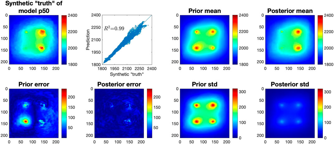
FIGURE 5. Evaluation of LIP-predicted CO₂ pressure after 10-years of injection based on 9 years of pressure observations in four wells. Top, left-right: synthetic “truth” of CO₂ pressure distribution (psi) in year 10 for model p50; cross-plot of the synthetic “truth” and LIP-predicted pressure distribution; mean pressure distribution (psi) from the prior samples; and LIP-estimated posterior mean after incorporating 9 years of observations; Bottom: absolute prediction error and the standard deviation (std) from the prior samples and LIP-generated posterior samples.

Following the similar steps, we applied the LIP method to the other two synthetic cases. Figure 6 shows the results for the p25 case. The figure indicates that the prior mean pressure map is dramatically deviated from the synthetic “truth” in this case. Because of the low porosity and permeability of the p25 geomodel, the pressure is relatively large, up to 2,800 psi around the injection wells. The prior mean significantly underestimates the pressure with a MAE of 108 psi and the prior estimate does not capture the pressure movement. On the other hand, the posterior mean produced by LIP not only accurately delineates the pressure front, but also identifies that the two wells at the bottom have larger pressure buildup, resulting in a smaller MAE of 42.27 psi. Compared to the prior, the posterior mean pressure field is much more like the synthetic “truth” with a R² of 0.96 and the posterior error field is also much smaller. Figure 7 summarizes the results of the p75 case. Due to the high porosity and permeability of the p75 geomodel, the pressure is relatively small in this case, below 2,100 psi. As the prior mean is an average of the other 99 geomodels, it significantly overestimates the pressure with a MAE of 75.4 psi. The LIP method, after effectively incorporating the observations from the four wells, dramatically reduces the MAE to 4.76 psi which is only 6.3% of the prior MAE. Furthermore, the posterior mean pressure field is very similar to the synthetic “truth” with a R² of 0.98 resulting in uniformly small posterior errors in the entire domain.

FIGURE 6

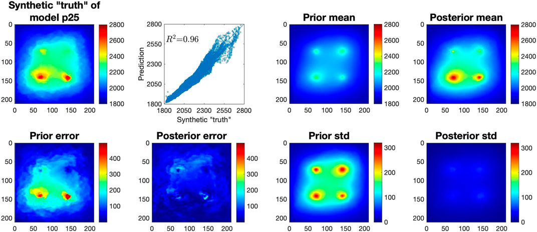
FIGURE 6. Evaluation of LIP-predicted CO₂ pressure after 10-years of injection based on 9 years of pressure observations in four wells. Top, left-right: synthetic “truth” of CO₂ pressure distribution (psi) in year 10 for model p25; cross-plot of the synthetic “truth” and LIP-predicted pressure distribution; mean pressure distribution (psi) from the prior samples; and LIP-estimated posterior mean after incorporating 9 years of observations; Bottom: absolute prediction error and the standard deviation (std) from the prior samples and LIP-generated posterior samples.

FIGURE 7

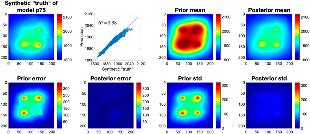
FIGURE 7. Evaluation of LIP-predicted CO₂ pressure after 10-years of injection based on 9 years of pressure observations in four wells. Top, left-right: synthetic “truth” of CO₂ pressure distribution (psi) in year 10 for model p75; cross-plot of the synthetic “truth” and LIP-predicted pressure distribution; mean pressure distribution (psi) from the prior samples; and LIP-estimated posterior mean after incorporating 9 years of observations; Bottom: absolute prediction error and the standard deviation (std) from the prior samples and LIP-generated posterior samples.

Although these three synthetic cases show dramatically different pressure distributions and patterns, e.g., within the region of pressure buildup caused by CO₂ injection, the difference between the cases of p25 and p75 is approximately 100–800 psi, all the cases indicate that the LIP method greatly improves estimation accuracy compared to the prior mean. Additionally, LIP significantly reduces the predictive uncertainty by producing a smaller posterior standard deviation field than the prior standard deviation field, which gives not only an accurate but also a confident forecasting. As shown in the last plots of Figures 5, 6, 7, the posterior standard deviation of the pressure field is close to zero in the entire domain. The resulted accurate and credible prediction of the CO₂ pressure distribution in the reservoir is critical for risk assessment and to inform decisions made by site operators.

To evaluate the LIP’s ability to incorporate additional observations for prediction improvement and to investigate the sensitivity of prediction performance to the number of observations, we designed a series of numerical experiments (Case I – Case V in Table 1) where we incorporate differing numbers of years of pressure data from the wells. The results of incorporating 1, 2, 5, and 7 years of observed data to predict pressure distribution in year 10 are presented in Figure 8. As shown in the figure, incorporating more years of observations produces a posterior mean pressure field that gets asymptotically closer to the synthetic “truth” in Figure 5. The MAE, as summarized in Table 1, gradually decreases from 14.85 psi (incorporating 1 year of data), to 11.59 psi (incorporating 2 years of data), to 10.77 psi (incorporating 5 years of data), to 8.05 psi (incorporating 7 years of data), and finally to 7.77 when incorporating 9 years of observations for forecasting. In incorporation of only 1 year of data, the posterior mean is already able to capture the major patterns and movement of the pressure field; additional years of data gradually refine the detail of the predicted pressure map. This indicates that the LIP method can effectively extract the information from the limited simulation data for learning the observation-prediction relationship and incorporates the observed data for updating the prediction from the unconstraint prior estimation to more accurate posterior estimation.

FIGURE 8

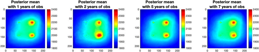
FIGURE 8. LIP estimated posterior mean of the CO₂ pressure distribution in year 1after considering 1, 2, 5, and 7 years of pressure observations (obs) in four wells. The synthetic “truth” is in Figure 5.

Note that the incorporation of these additional observations in LIP does not require extra reservoir simulations. LIP incorporates new observation data by performing the analysis in Steps 2-4 of Section 2 based on the corresponding observation variable simulations from the prior sample set. The statistical analysis in Steps 2-4 is very fast which takes a few seconds in this study. The ability of LIP to rapidly generate new forecasts promises fast integration of streaming observations for timely forecasts in field operation. Furthermore, the additional data are not necessarily the transient data from the same well with a longer period of observations, they can also come from other wells and can be different types of measurements. As long as these additional observation variables have been simulated in the forward runs, there is no need to perform extra simulations when incorporating the new data.

In addition to predicting the pressure distribution, we also applied the LIP method to predict the CO₂ plume in the storage reservoir. Figure 9 shows the prediction results of CO₂ distribution in year 10 after incorporating 9 years of observations from the four wells for the three synthetic cases. The three cases show dramatically different CO₂ distributions, e.g., within the footprint of the CO₂ plume, the difference in gas saturation between the cases of p25 and p75 is approximately ±0.35. Despite the significantly diverse CO₂ distributions, the posterior mean produced by LIP can still capture their major patterns. The prior mean shows that the footprints of CO₂ around the four wells are similar to each other, however, the posterior mean from LIP depicts that the CO₂ plume is actually different around different wells and the resulting patterns are much closer to the synthetic “truth”. Additionally, the prior samples display a large standard deviation around the wells. After effectively incorporating the observations, the posterior standard deviation is greatly reduced, showing more confident prediction. Although LIP improved the prediction accuracy and credibility by producing a better posterior mean and a smaller standard deviation than the prior estimation, its prediction of CO₂ plume is relatively poor compared to the prediction of pressure distributions, where the posterior pressure field is more like the synthetic “truth”. One reason is that CO₂ field is less continuous than the pressure field, i.e., the pressure field extends outwards from each of the four wells and forms a continuous extent that covers most of the model domain, whereas the CO₂ plumes around each of the four wells are smaller in extent and more irregularly shaped. So after dimensional reduction, the CO₂ plume may lose more information for statistical learning. Moreover, the observation-prediction relationship of CO₂ gas saturation is more complicated than the relationship of the pressure, and the current study is limited to 99 training samples for learning the relationship which may not be enough. Additionally, we only have observations from the four wells at 31 time steps; these limited simulation data and point observed data are far less than enough to accurately delineate the CO₂ footprint in such a large and heterogeneous domain.

FIGURE 9

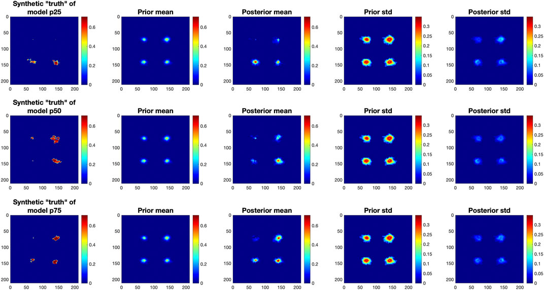
FIGURE 9. Evaluation of LIP-predicted CO₂ plume after 10-years of injection based on 9 years of saturation observations in four wells. Three rows are results for the three different synthetic models where model p25, p50, and p75 correspond to low, mid, and high porosity, respectively. Left-right: synthetic “truth” of CO₂ plume; mean pressure distribution (psi) from the prior samples; LIP-estimated posterior mean after incorporating 9 years of observations; and the standard deviation (std) from the prior samples and LIP-generated posterior samples.

4 Discussion

In this paper, we provide an efficient and effective prediction method (LIP)—using a set of machine learning techniques—to perform accurate, timely forecasts for geological carbon storage based on a limited number of measurements and a few model simulations. We use three different synthetic cases demonstrate that the LIP method can greatly improve CO₂ plume and pressure prediction accuracy and reduce predictive uncertainty by effectively incorporating observations. The proposed LIP method runs very fast; after obtaining prior samples, it takes a few seconds to perform the entire process—from dimension reduction, to canonical correlation analysis, to Bayesian inference for prediction. The prior samples are independent and can be performed completely concurrently on parallel computing platforms; with enough processors available, the generation of the hundred prior samples would only require the same wallclock time as one forward reservoir simulation. LIP is also data efficient; based on 99 prior samples, it can effectively learn the observation-prediction relationship and accurately infer the posterior prediction distributions by incorporating the observed data. LIP uses estimated observation-prediction relationship to infer predictions. In this study, we used PCA followed by CCA to build a linear relationship in the reduced canonical space and then use the Gaussian linear regression for predictions. In situations when the relationship is nonlinear and multimodal, we can use Bayesian neural networks for regression. To avoid extrapolation, LIP requires the observation data to lie inside of the prior samples. We can adjust the prior distribution and increase the prior sample size to satisfy this requirement.

LIP has a considerable potential to fundamentally change how timely decisions are made about CO₂ storage operations. Bypassing the conventional workflow of history matching and then forward simulations, LIP provides fast updating forecasts of CO₂ plume and pressure distributions from streaming observations, thus providing operators with early warning of off-normal behavior and more time to implement mitigation measures. In our future work, we will apply LIP to real measurement data from the field, and deploy it to CO₂ storage operators for fast decision making.

Data Availability Statement

The raw data supporting the conclusions of this article will be made available by the authors, without undue reservation.

Author Contributions

DL developed the algorithms, planned and implemented the numerical experiments, and led manuscript preparation. SP contributed to the research plan, interpretation of results, and manuscript preparation. NA, MB-K, TJ, and CW generated the geomodels, performed the reservoir simulations, and helped prepare the manuscript.

Funding

Primary funding support for this work is provided by the Science-informed Machine Learning to Accelerate Real Time decision making for Carbon Storage (SMART-CS) Initiative, funded by the US Department of Energy (DOE), Office of Fossil Energy. Additional support is provided by the Artificial Intelligence Initiative as part of the Laboratory Directed Research and Development Program of Oak Ridge National Laboratory, managed by UT-Battelle, LLC, for the US DOE under contract DE-AC05-00OR22725. This research is also sponsored by the Data-Driven Decision Control for Complex Systems (DnC2S) project funded by the US DOE, Office of Advanced Scientific Computing Research.

Author Disclaimer

The United States Government retains and the publisher, by accepting the article for publication, acknowledges that the United States Government retains a non-exclusive, paidup, irrevocable, world-wide license to publish, or reproduce the published form of this manuscript, or allow others to do so, for United States Government purposes.

Conflict of Interest

Authors DL and SP were employed by Oak Ridge National Laboratory.

The remaining authors declare that the research was conducted in the absence of any commercial or financial relationships that could be construed as a potential conflict of interest.

Publisher’s Note

All claims expressed in this article are solely those of the authors and do not necessarily represent those of their affiliated organizations, or those of the publisher, the editors and the reviewers. Any product that may be evaluated in this article, or claim that may be made by its manufacturer, is not guaranteed or endorsed by the publisher.

Acknowledgments

Part of the methodology of this manuscript has been presented at the 2019 International Conference on Data Mining Workshops, DOI: 10.1109/ICDMW.2019.00049. This manuscript has been co-authored by staff from UT-Battelle, LLC under Contract No. DE-AC05-00OR22725 with the U.S. Department of Energy.

References

Alcalde, J., Flude, S., Wilkinson, M., Johnson, G., Edlmann, K., Bond, C. E., et al. (2018). Estimating Geological CO2 Storage Security to Deliver on Climate Mitigation. Nat. Commun. 9, 2201. doi:10.1038/s41467-018-04423-1

PubMed Abstract | CrossRef Full Text | Google Scholar

Bianco, A., Cominelli, A., Dovera, L., Naevdal, G., and Valles, B. (2007). “History Matching and Production Forecast Uncertainty by Means of the Ensemble Kalman Filter: A Real Field Application,” in EUROPEC/EAGE Conference and Exhibition, London, United Kingdom, June 2007. SPE-107161-MS. doi:10.2118/107161-MS

CrossRef Full Text | Google Scholar

Bosshart, N. W., Azzolina, N. A., Ayash, S. C., Peck, W. D., Gorecki, C. D., Ge, J., et al. (2018). Quantifying the Effects of Depositional Environment on Deep saline Formation Co2 Storage Efficiency and Rate. Int. J. Greenhouse Gas Control. 69, 8–19. doi:10.1016/j.ijggc.2017.12.006

CrossRef Full Text | Google Scholar

Brandt, A. R., Heath, G. A., Kort, E. A., O'Sullivan, F., Petron, G., Jordaan, S. M., et al. (2014). Methane Leaks from north American Natural Gas Systems. Science 343, 733–735. doi:10.1126/science.1247045

PubMed Abstract | CrossRef Full Text | Google Scholar

Cavanagh, A., and Wildgust, N. (2011). Pressurization and Brine Displacement Issues for Deep saline Formation Co2 Storage. Energ. Proced. 4, 4814–4821. 10th International Conference on Greenhouse Gas Control Technologies. doi:10.1016/j.egypro.2011.02.447

CrossRef Full Text | Google Scholar

Celia, M. A., Bachu, S., Nordbotten, J. M., and Bandilla, K. W. (2015). Status of CO2storage in Deep saline Aquifers with Emphasis on Modeling Approaches and Practical Simulations. Water Resour. Res. 51, 6846–6892. doi:10.1002/2015wr017609

CrossRef Full Text | Google Scholar

Celia, M., Bachu, S., Nordbotten, J., Gasda, S., and Dahle, H. (2005). “Quantitative Estimation of CO2 Leakage from Geological storageAnalytical Models, Numerical Models, and Data Needs,” in Greenhouse Gas Control Technologies 7. Editors E. Rubin, D. Keith, C. Gilboy, M. Wilson, T. Morris, J. Galeet al. (Oxford: Elsevier Science Ltd), 663–671. doi:10.1016/B978-008044704-9/50067-7

CrossRef Full Text | Google Scholar

Chen, B., Harp, D. R., Lu, Z., and Pawar, R. J. (2020). Reducing Uncertainty in Geologic Co2 Sequestration Risk Assessment by Assimilating Monitoring Data. Int. J. Greenhouse Gas Control. 94, 102926. doi:10.1016/j.ijggc.2019.102926

CrossRef Full Text | Google Scholar

Daoud, J. I. (2017). Multicollinearity and Regression Analysis. J. Phys. Conf. Ser. 949, 012009. doi:10.1088/1742-6596/949/1/012009

CrossRef Full Text | Google Scholar

Doughty, C., and Oldenburg, C. M. (2020). Co2 Plume Evolution in a Depleted Natural Gas Reservoir: Modeling of Conformance Uncertainty Reduction over Time. Int. J. Greenhouse Gas Control. 97, 103026. doi:10.1016/j.ijggc.2020.103026

CrossRef Full Text | Google Scholar

Gorecki, C. D., Sorensen, J. A., Bremer, J. M., Knudsen, D., Smith, S. A., Steadman, E. N., et al. (2009). “Development of Storage Coefficients for Determining the Effective Co2 Storage Resource in Deep saline Formations,” in SPE International Conference on CO2 Capture, Storage, and Utilization, San Diego, CA, November 2009. doi:10.2118/126444-MS

CrossRef Full Text | Google Scholar

Guo, B., Bandilla, K. W., Doster, F., Keilegavlen, E., and Celia, M. A. (2014). A Vertically Integrated Model with Vertical Dynamics for CO2storage. Water Resour. Res. 50, 6269–6284. doi:10.1002/2013WR015215

CrossRef Full Text | Google Scholar

Humez, P., Audigane, P., Lions, J., Chiaberge, C., and Bellenfant, G. (2011). Modeling of CO2 Leakage up through an Abandoned Well from Deep Saline Aquifer to Shallow Fresh Groundwaters. Transp Porous Med. 90, 153–181. doi:10.1007/s11242-011-9801-2

CrossRef Full Text | Google Scholar

Ji, X., and Zhu, C. (2015). “CO2 Storage in Deep Saline Aquifers,” in Novel Materials for Carbon Dioxide Mitigation Technology. Editors F. Shi, and B. Morreale (Amsterdam: Elsevier), 299–332. doi:10.1016/b978-0-444-63259-3.00010-0

CrossRef Full Text | Google Scholar

Lu, D., Ricciuto, D., Walker, A., Safta, C., and Munger, W. (2017). Bayesian Calibration of Terrestrial Ecosystem Models: a Study of Advanced Markov Chain Monte Carlo Methods. Biogeosciences 14, 4295–4314. doi:10.5194/bg-14-4295-2017

CrossRef Full Text | Google Scholar

Metz, B., Davidson, O., De Coninck, H., Loos, M., and Meyer, L. (2005). IPCC Special Report on Carbon Dioxide Capture and Storage. Cambridge: Cambridge University Press.

Google Scholar

Namhata, A., Oladyshkin, S., Dilmore, R. M., Zhang, L., and Nakles, D. V. (2016). Probabilistic Assessment of above Zone Pressure Predictions at a Geologic Carbon Storage Site. Sci. Rep. 6, 1–12. doi:10.1038/srep39536

PubMed Abstract | CrossRef Full Text | Google Scholar

Oliver, D. S., and Chen, Y. (2011). Recent Progress on Reservoir History Matching: a Review. Comput. Geosci. 15, 185–221. doi:10.1007/s10596-010-9194-2

CrossRef Full Text | Google Scholar

Pacala, S., and Socolow, R. (2004). Stabilization Wedges: Solving the Climate Problem for the Next 50 Years with Current Technologies. Science 305, 968–972. doi:10.1126/science.1100103

PubMed Abstract | CrossRef Full Text | Google Scholar

Pawar, R. J., Watson, T. L., and Gable, C. W. (2009). Numerical Simulation of Co2 Leakage through Abandoned wells: Model for an Abandoned Site with Observed Gas Migration in alberta, canada. Energ. Proced. 1, 3625–3632. doi:10.1016/j.egypro.2009.02.158

CrossRef Full Text | Google Scholar

Qiao, T., Hoteit, H., and Fahs, M. (2021). Semi-analytical Solution to Assess Co2 Leakage in the Subsurface through Abandoned wells. Energies 14, 2452. doi:10.3390/en14092452

CrossRef Full Text | Google Scholar

Yang, X., Liu, W., Liu, W., and Tao, D. (2021). A Survey on Canonical Correlation Analysis. IEEE Trans. Knowl. Data Eng. 33, 2349–2368. doi:10.1109/TKDE.2019.2958342

CrossRef Full Text | Google Scholar