Numerical evaluation of thermal and hydrodynamic effects caused by heat production well on geothermal Phlegraean Fields

1 Introduction

In recent years, there has been a growing worldwide trend toward the use of areas with high geothermal potential for electricity and hot water production, as reported in Bertani, 2015 and Bertani, 2007. The most recent geothermal energy research studies are focusing on the use of closed-loop plants which produce heat without geo-fluid extraction. These technologies are deep borehole heat exchangers (DBHEs), made up of a set of coaxial pipes which extract heat by conduction. The use of deep borehole heat exchangers has been studied by Nalla et al., 2005, Kujawa et al., 2006, Davis and Michaelides, 2009, Templeton et al., 2014, Noorollahi et al., 2015, Alimonti et al., 2018, Westaway 2018, and Renaud et al., 2019, with different analytical and numerical models, thus demonstrating the feasibility of the plant, although with low effectiveness of heat extraction, with respect to the geo-fluid extraction for conventional wells. These studies assessed the amount of heat and energy that DBHEs could produce in small geothermal reservoir areas. Nevertheless, the authors have not investigated the response of the reservoirs to heat extraction and the consequent change in the thermo-hydraulic characteristics of the studied domain. This type of study is a very complex analysis, and it is founded on thermo-fluid dynamic laws, written in the form of a non-linear high-order coupled partial differential equation system. Different spatial discretization schemes are presented in the literature generally based on the finite difference method (FDM) and finite element method (FEM). The common numerical solutions used include the Il’in Method (Il’in, 1969) which is implemented in the SHEMAT solver (Clauser, 2003), the Network Simulation Method (Cánovas et al., 2017) for dimensionless numerical problems, and the Galerkin Method (GM) for solving the system of partial differential equations (Gupta and Meek, 2002). An example of the last method applied to shallow enthalpy reservoirs can be found in Luo et al., 2003. During the solving process, some simplifications are considered, including physical phenomena and their characteristic parameters. An example is the well-known Boussinesq approximation. Furthermore, when evaluating the physical parameters of porous media, Bejan and Kraus, 2003 assumed average parameter values. At the same time, for an accurate estimate of the physical response of the system, some researchers such as Yusa, 1983, Holzbecher and Yusa, 1995, and Elder et al., 2017 studied the solution of the theoretical problems using dimensionless and normalized variables to identify whether a common behavior or dependency can exist between parameter and reservoir response. Such studies assume the stream function field as a representative value.

In this paper, an innovative software based on the GM has been developed using a hard set of numerical simulations of the geothermal reservoir of the Phlegraean Fields, a volcanic area located in the Campania Region, Italy. This software is adapted to simulate the geothermal reservoirs and estimate the temperature, stream function, and velocity components of the fluid by solving the momentum and energy equations both with and without a deep borehole heat exchanger in service. This integrated calculation code (reservoir–DBHE) enables the evaluation of the effect of closed-well extraction on the thermal and hydrodynamic rebalancing of the reservoir. In fact, the domain is in a quasi-steady state before the DBHE goes into service. When the DBHE system is in service, it is shows better accuracy of the solution, considering the rebalancing effects of the temperature and hydrodynamic characteristics of the domain on the DBHE and not fixing “a priori” areas of influence or temporally constant temperature values.

2 Governing physical laws and the mathematical model

2.1 Governing physical laws

The solved equation system is based on the fluid flow mass conservation Eq. 1, the energy conservation, and the momentum conservation laws (Eqs. 2, 3) combined with the Darcy law. According to Bejan and Kraus, 2003, the energy conservation equation is applied to a porous medium while taking into account a local thermal equilibrium between the solid part, s, and the fluid part, f, contained in the pores, i.e., T_s = T_f = T. In this case, heat conduction occurs simultaneously in the solid and fluid phases. Radiative effects, viscous dissipation, and the work carried out by the pressure change are negligible (Bejan and Kraus, 2003).

$\frac{\partial v_z}{\partial z}+\frac{\partial v_x}{\partial x}=0.(1)$

$\sigma \frac{\partial T}{\partial t}+v_x\frac{\partial T}{\partial x}+v_z\frac{\partial T}{\partial z}-\frac{k_{m,x}}{{\left(\rho c\right)}_f}\frac{{\partial }^{2}T}{\partial x^2}-\frac{k_{m,z}}{{\left(\rho c\right)}_f}\frac{{\partial }^{2}T}{\partial z^2}=0.(2)$

$\frac{K_z}{K_x}\frac{\partial v_z}{\partial x}-\frac{\partial v_x}{\partial z}-\frac{K_{z}g}{\mu }\frac{\partial \rho }{\partial T}\frac{\partial T}{\partial x}=0.(3)$

Some approximations are used by authors such as Yusa, 1983, Holzbecher and Yusa, 1995, and Bejan and Kraus, 2003 to simplify this system of partial differential equations. The Boussinesq approximation reported in Eqs 4, 5 is an important assumption related to the density change of water due to the change in the temperature.

$\rho -{\rho }_0=-{\rho }_0\beta \left(T-T_0\right),(4)$

$\mathrm{\Delta }\rho =-{\rho }_0\beta \mathrm{\Delta }T,(5)$

where σ is the ratio between specific heats proportional to the system’s porosity ϕ; k_m,x and k_m,z are the overall thermal conductivity in the x and z directions (horizontal and vertical), respectively; K_x and K_z are the horizontal and vertical hydraulic permeabilities of the soils, respectively; g is the gravity acceleration; μ and β are, respectively, the fluid dynamic viscosity and the thermal expansion coefficient of the water which are the function of the nodal values of temperature and pressure, T_n and P_n nodal (n) values. The water density is represented by ρ and ρ₀, with the subscript of 0 referring to the reference temperature. Then, the momentum equation can be written as follows (Eq. 6).

$\frac{K_z}{K_x}\frac{\partial v_z}{\partial x}-\frac{\partial v_x}{\partial z}+\frac{K_{z}g{\rho }_0\beta \left(T_n,P_n\right)}{\mu \left(T_n,P_n\right)}\frac{\partial T}{\partial x}=0.(6)$

The system’s closure equation is the continuity equation by the definition of the stream function field (ψ) as defined by Eqs 7, 8 (Holzbecher, 1998).

$v_x=-\frac{\partial \psi }{\partial z}.(7)$

$v_z=\frac{\partial \psi }{\partial x}.(8)$

By substituting Eqs 7, 8 with Eqs 2, 6, we obtain the final system χ_Ω(T, ψ, v_x, v_z) integrated by the two-system closure parameters β and μ as follows:

${\chi }_{\mathrm{\Omega }}\left(T,\psi ,v_x,v_z\right)=\left\{,\begin{array}{c}\sigma \frac{\partial T}{\partial t}-\frac{\partial \psi }{\partial z}\frac{\partial T}{\partial x}+\frac{\partial \psi }{\partial x}\frac{\partial T}{\partial z}-\frac{k_{m,x}}{{\left(\rho c\right)}_f}\frac{{\partial }^{2}T}{\partial x^2}-\frac{k_{m,z}}{{\left(\rho c\right)}_f}\frac{{\partial }^{2}T}{\partial z^2}=0\hfill \\ \frac{K_z}{K_x}\frac{{\partial }^2\psi }{\partial x^2}+\frac{{\partial }^2\psi }{\partial z^2}+\frac{K_{z}g{\rho }_0\beta \left(T_n,P_n\right)}{\mu \left(T_n,P_n\right)}\frac{\partial T}{\partial x}=0\hfill \\ v_x+\frac{\partial \psi }{\partial z}=0\hfill \\ v_z-\frac{\partial \psi }{\partial x}=0\hfill \\ \beta \left(T,P\right)=Closingequationparameter\hfill \\ \mu \left(T,P\right)=Closingequationparameter\hfill \end{array}.\right.(9)$

The effects of the DBHE on the domain and the resulting temperature changes are defined using the following function (Ramey, 1962) (Cheng et al., 2011):

${\chi }_{wb}\left(T\right)={\left.\frac{\partial Q}{\partial z}\right|}_{wb}-\frac{2\pi k_{ei}}{f{\left(t\right)}^{*}}\left(T_{wb}-T_{ei}\right),(10)$

where T_ei is the formation temperature, T_wb is the external temperature of the well’s wall, ∂Q/∂z is the DBHE heat loss or rate along dz, and the term f(t)* is the dimensionless transient heat conduction defined by Cheng et al., 2011 as follows:

$f{\left(t\right)}^{*}=\ln \left(2\sqrt{{\tau }_d}\right)-\frac{C_1}{2}+\frac{1}{4{\tau }_d}\left[1+\left(1-\frac{1}{\omega }\right)\ln \left(4{\tau }_d\right)+C_1\right].(11)$

In Eq. 11, τ_d is the dimensionless time, ω is the ratio between the heat capacities of the formation and the DBHE, and C₁ is Euler’s constant. The dimensional parameters and properties of the DBHE contained in τ_d and ω are derived from the work of Cheng et al., 2011, Le Nian et al., 2014, and Tang et al., 2019.

2.2 Mathematical model

The continuous domain is discretized using finite elements with four nodes and linear shape functions, and the GM is used to solve the system of nonlinear partial differential equations (PDEs). An implicit difference scheme is used to discretize the time derivative term. The multivariable matrix system associated with the domain Ω and its solution χ is given below.

${\chi }_{\mathrm{\Omega }}\left(T,\psi ,v_x,v_z\right)=\left\{,\begin{array}{c}\left[P\right]\left\{T\left(t\right)\right\}+\left(-\left[B_1\right]+\left[B_2\right]+\left[I_1\right]+\left[I_2\right]\right)\left\{T\right\}+\left\{Z\right\}=0\hfill \\ \left(\left[S\right]+\left[D\right]\right)\left\{\psi \right\}+\left\{Y\right\}+\left[R\right]\left\{T\right\}=0\hfill \\ \left[V\right]\left\{v_x\right\}+\left[M\right]\left\{\psi \right\}=0\hfill \\ \left[V\right]\left\{v_z\right\}-\left[L\right]\left\{\psi \right\}=0\hfill \\ \beta \left(T,P\right)=Closingequationparameter\hfill \\ \mu \left(T,P\right)=Closingequationparameter\hfill \end{array}.\right.(12)$

The matrices of the previous system of equations are defined as follows for a generic domain element e with weight function N_L and L number of weight function nodes (L, i = 1, 2 … 4):

$\begin{array}{ll}\hfill \left[P^e\right]\left\{T_i\left(t\right)\right\}& ={\int }_e\tilde{\sigma }\left[N_L\right]\left[N_i\right]de\left\{T_i\left(t\right)\right\}\hfill \\ \hfill & ={\int }_{x_a}^{x_b}{\int }_{z_a}^{z_b}\tilde{\sigma }\left[N_L\right]\left[N_i\right]dxdz\frac{\left\{T_i^{\mathrm{\Delta }t+t}-T_i^t\right\}}{\mathrm{\Delta }t}\hfill \end{array}(13)$

$\begin{array}{ll}\hfill \left[B_1^e\right]& ={\int }_e\left[N_L\right]\left[\frac{\partial N_i}{\partial z}\right]\left\{\psi \right\}\left[\frac{\partial N_i}{\partial x}\right]de\hfill \\ \hfill & ={\int }_{x_a}^{x_b}{\int }_{z_a}^{z_b}\left[N_L\right]\left[\frac{\partial N_i}{\partial z}\right]\left\{\psi \right\}\left[\frac{\partial N_i}{\partial x}\right]dxdz\hfill \end{array}(14)$

$\begin{array}{ll}\hfill \left[B_2^e\right]& ={\int }_e\left[N_L\right]\left[\frac{\partial N_i}{\partial x}\right]\left\{\psi \right\}\left[\frac{\partial N_i}{\partial z}\right]de\hfill \\ \hfill & ={\int }_{x_a}^{x_b}{\int }_{z_a}^{z_b}\left[N_L\right]\left[\frac{\partial N_i}{\partial x}\right]\left\{\psi \right\}\left[\frac{\partial N_i}{\partial z}\right]dxdz\hfill \end{array}(15)$

$\begin{array}{ll}\hfill \left[I_1^e\right]& ={\int }_e{\tilde{\alpha }}_{m,x}\left[\frac{\partial N_L}{\partial x}\right]\left[\frac{\partial N_i}{\partial x}\right]de\hfill \\ \hfill & ={\int }_{x_a}^{x_b}{\int }_{z_a}^{z_b}{\tilde{\alpha }}_{m,x}\left[\frac{\partial N_L}{\partial x}\right]\left[\frac{\partial N_i}{\partial x}\right]dxdz\hfill \end{array}(16)$

$\begin{array}{ll}\hfill \left[I_2^e\right]& ={\int }_e{\tilde{\alpha }}_{m,z}\left[\frac{\partial N_L}{\partial z}\right]\left[\frac{\partial N_i}{\partial z}\right]de\hfill \\ \hfill & ={\int }_{x_a}^{x_b}{\int }_{z_a}^{z_b}\widetilde{{\alpha }_{m,z}}\left[\frac{\partial N_L}{\partial z}\right]\left[\frac{\partial N_i}{\partial z}\right]dxdz\hfill \end{array}(17)$

$\left\{Z^e\right\}={\oint }_l{\left\{q_i^e\right\}}^T\left[N_L\right]\left\{\tilde{n}\right\}dl.(18)$

$\begin{array}{ll}\hfill \left[S^e\right]& ={\int }_e\frac{\widetilde{K_z}}{\widetilde{K_x}}\left[\frac{\partial N_L}{\partial x}\right]\left[\frac{\partial N_i}{\partial x}\right]de\hfill \\ \hfill & ={\int }_{x_a}^{x_b}{\int }_{z_a}^{z_b}\frac{\widetilde{K_z}}{\widetilde{K_x}}\left[\frac{\partial N_L}{\partial x}\right]\left[\frac{\partial N_i}{\partial x}\right]dxdz\hfill \end{array}(19)$

$\begin{array}{ll}\hfill \left[D^e\right]& ={\int }_e\left[\frac{\partial N_L}{\partial z}\right]\left[\frac{\partial N_i}{\partial z}\right]de\hfill \\ \hfill & ={\int }_{x_a}^{x_b}{\int }_{z_a}^{z_b}\left[\frac{\partial N_L}{\partial z}\right]\left[\frac{\partial N_i}{\partial z}\right]dxdz\hfill \end{array}(20)$

$\left\{Y^e\right\}=-\tilde{K}{\oint }_l{\left\{Q_i^e\right\}}^T\left[N_L\right]\left\{\tilde{n}\right\}dl.(21)$

$\begin{array}{ll}\hfill \left\{R^e\right\}& ={\int }_e\frac{K_{z}g{\rho }_0\beta \left(T_n,P_n\right)}{\mu \left(T_n,P_n\right)}\left[N_L\right]\left[\frac{\partial N_i}{\partial x}\right]de\hfill \\ \hfill & ={\int }_{x_a}^{x_b}{\int }_{z_a}^{z_b}\frac{K_{z}g{\rho }_0\beta \left(T_n,P_n\right)}{\mu \left(T_n,P_n\right)}\left[N_L\right]\left[\frac{\partial N_i}{\partial x}\right]dxdz\hfill \end{array}(22)$

$\left\{V^e\right\}={\int }_e\left[N_L\right]\left[N_i\right]de={\int }_{x_a}^{x_b}{\int }_{z_a}^{z_b}\left[N_L\right]\left[N_i\right]dxdz(23)$

$\left\{M^e\right\}={\int }_e\left[N_L\right]\left[\frac{\partial N_i}{\partial z}\right]de={\int }_{x_a}^{x_b}{\int }_{z_a}^{z_b}\left[N_L\right]\left[\frac{\partial N_i}{\partial z}\right]dxdz.(24)$

$\left\{L^e\right\}={\int }_e\left[N_L\right]\left[\frac{\partial N_i}{\partial x}\right]de={\int }_{x_a}^{x_b}{\int }_{z_a}^{z_b}\left[N_L\right]\left[\frac{\partial N_i}{\partial x}\right]dxdz.(25)$

In the previous equation, $\{\tilde{n}\}$ is an outer normal to the element’s boundary. The heat flux vector {q} and the primitive of the stream function {F} are both discretized as follows:

$\left\{q^e\right\}=-\tilde{k}\left[B\right]\left\{T_i\right\},(26)$

$\left\{F^e\right\}=\left[B\right]\left\{{\psi }_i\right\},(27)$

where [B] is the matrix containing the shape functions’ first derivatives in the x and z directions. For the physical parameters, $\tilde{k}$ represents thermal conductivity, $\widetilde{K_x}$ and $\widetilde{K_z}$ are the hydraulic permeabilities, and $\tilde{\sigma }$, $\widetilde{{\alpha }_{m,x}}$, and $\widetilde{{\alpha }_{m,z}}$ represent heat capacity ratio and diffusivity, respectively, as constant tensor matrices in the x and z directions. Different transient analyses are developed, at first, to define the temperature and flow fields in the geothermal reservoir, and an analysis is performed without the DBHE. After this simulation reaches a steady state, a similar transient analysis with the borehole well is performed. Temperature variation at the DBHE’s external surface is discretized and nodally replaced in the (12) system as follows:

$\begin{array}{ll}\hfill \chi \left(T_i,t\right)& ={\int }_{x_a}^{x_b}{\int }_{z_a}^{z_b}{k}_{ei}{A}_{wb}\left[\frac{\partial N_L}{\partial z}\right]\left[\frac{\partial N_i}{\partial z}\right]\left\{T_{wb}\right\}\hfill \\ \hfill & -\frac{2\pi k_{ei}}{f{\left(t\right)}^{*}}\left[N_L\right]\left[N_i\right]\left\{T_{wb}-T_{ei}\right\}dxdz\hfill \end{array}(28)$

where, in the integrals, the interval [a, b] represents the generic points of the discretized element.

3 Computation

3.1 Domain and analysis computation

The implemented geothermal reservoir, depicted in Figure 1 (the red line), is located in the Campi Fregrei volcanic area, near Lake Averno and Baia di Pozzuoli, in the area known as “Mofete.” From 1930 to 1980, several deep exploration wells were drilled in this zone for hypothetic hydrocarbon exploration. We found indications of the main temperatures measured up to a depth of 2,000 m for wells “MF1” and “MF2,” stratigraphy, and examples of 3D modeling in the studies conducted by Carlino et al., 2012 and Carlino et al., 2016.

FIGURE 1

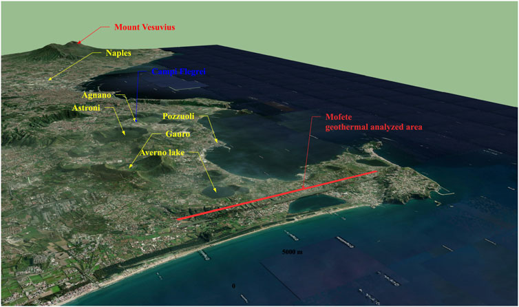
FIGURE 1. 3D view of the geothermally analyzed area in Naples, Italy.

The geothermal domain, with 6,000 m longitude and a 3,000 m elevation, extended in the x and z directions, is modeled by a non-uniform grid of 82 × 31 nodes (coordinates are given in Supplementary Table S1). The study of Troise et al., 2001 was referenced for a two-dimensional domain, and the depth of the geological layers was deduced from the study of Carlino et al., 2016, implementing six layers with anisotropic parameters along the z direction, as shown in Figure 2.

FIGURE 2

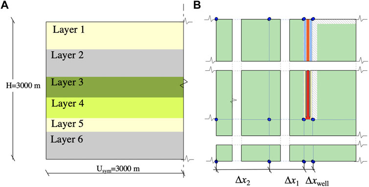
FIGURE 2. Geometrical dimension of the implemented reservoir-layer [(A) symmetrical along x] and DBHE (B).

Table 1 contains the numerical values used in the simulation. The hydraulic permeability, thermal conductivity, density, and specific heat of the soil were determined using Carlino et al., 2016, and porosity was determined using Troise et al., 2001.

TABLE 1

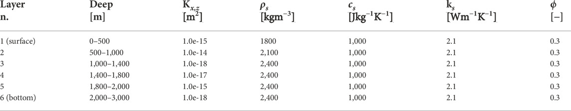
TABLE 1. Hydraulic and thermal model parameters are implemented.

The DBHE depicted in Figure 3 was implemented and simulated in the second part of the study. The well is located in the center of the geothermal reserve and has a depth of 2,000 m. The geometric and thermal properties of the DBHE were derived from the study conducted by Le Nian et al., 2014, while the thermal diffusivity and thermal conductivity of the formation were, respectively, altered to 3.9634e—07 [m² × s⁻¹] and 2.1 [W × m⁻¹ × K⁻¹]. The particularity of our study is that the nodal temperature next to the DBHE (i.e., in the formation) is time-dependent and changes in the domain for each analysis step rather than being imposed as a constant.

FIGURE 3

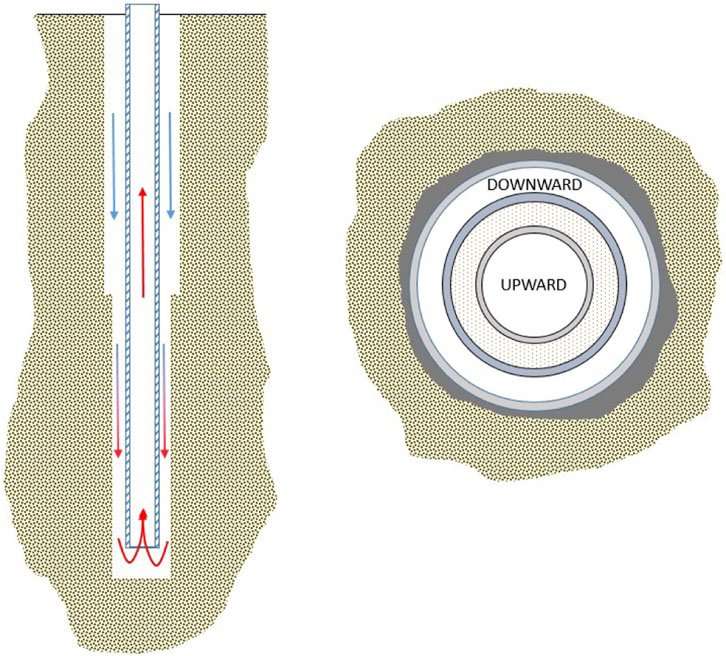
FIGURE 3. Schematic of a DBHE.

The developed code includes a special non-linear function for defining water’s dynamic viscosity μ(T_n; P_n) and the thermal expansion coefficient β(T_n; P_n) represented in Figures 4, 5, respectively. The data are modeled by Mifofski, 2013 in a MATLAB, 2018 function linked to the nodal variables T_n and P_n, which stand for the temperature and pressure in the control node, n, respectively The information is derived from the IAPWS, 2007 formulation. The ranges of the nodal temperature and pressure variations are between [0, 700°C] and [0, 50 MPa], respectively.

FIGURE 4

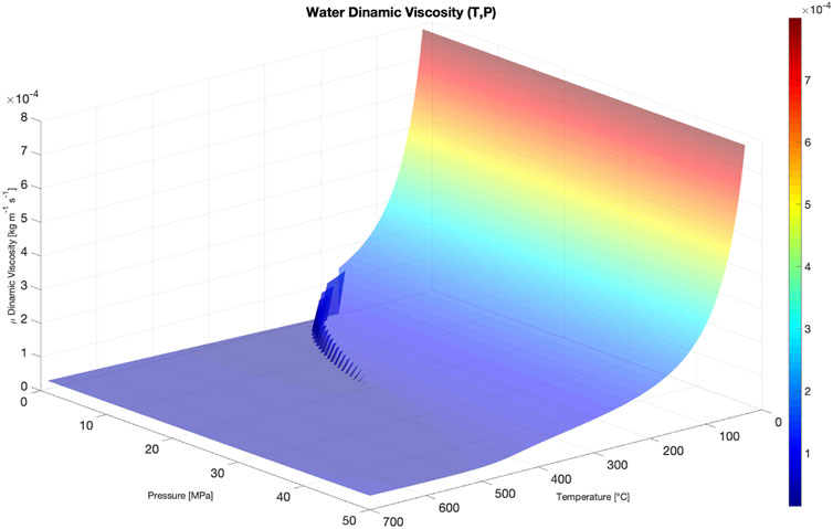
FIGURE 4. Pattern of the implemented dynamic viscosity of water [kg × m⁻¹ × s⁻¹].

FIGURE 5

FIGURE 5. Pattern of the implemented thermal expansion coefficient of water [°C⁻¹].

Using a dynamic computational time-step whose value depends on the convergence and efficiency of the solution, a transient analysis is performed (see Supplementary Material; Section 2). The initial time-step Δt and the final simulation instant trend are equal to 1.00e+10 (s) and 5.00e+13 (s), respectively. Effects of the presence of a DBHE in the geothermal reservoir are then investigated. For this case, the final analysis time (t_DBHEend) is 200 years.

3.2 Computational initial and boundary conditions

To simulate the heat source and the groundwater flow shown in Figure 6 and described in Table 2, severe initial and boundary conditions are implemented. The boundary conditions are of Neumann and Dirichlet types (Holzbecher, 1998). The heat source reservoir is idealized with nodal temperature values that increase in the x-direction and are constant in time. In the center of the reservoir, where the magmatic source is located, the temperature can reach a maximum of 400°C. The temperature isolines reported in the conceptual model of the geothermal reservoir (Carlino et al., 2016) based on data inferred from drilling and production tests are used to determine the heat source configuration (and its maximum temperature). In fact, given a vertical reference, the trend of the temperature isolines in this scheme is parabolic, with temperature reduction traveling outward from the geothermal reservoir’s center. Comparing this scheme to the one modeled by Troise et al., 2001 to define the effects of the magma chamber simulation, the maximum presumed temperature value is near 400°C. The nodal function χ(T_n) is described in Eq. 29, and its values are reported in Table 2. A second-order forward difference scheme is used to implement a null heat flux boundary condition (q = 0 [W × m⁻²]) at the lateral walls (Eq. 30). This implementation considers the potential existence of additional thermal sources outside the discretized domain that might cause symmetrically repeating effects. Finally, a constant temperature of 35°C has been considered for the domain’s top boundary. Except for the base of the reservoir, the same value is applied for the entire domain Ω.

$\chi \left(T_n\right)=T_n-T_{{\mathrm{\Gamma }}_{\left(\mathrm{1,2,3,4,5}\right)}}inthebottonandtopofthedomain.(29)$

$\chi \left(T_n\right)=\frac{3T_i-4T_{i+1}+T_{i+2}}{2\mathrm{\Delta }x}forthelateralwalls.(30)$

FIGURE 6

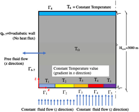
FIGURE 6. Representation of the main boundary and initial condition of the domain.

TABLE 2

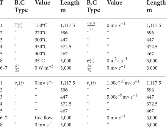
TABLE 2. Initial and boundary conditions applied to the symmetrical half-domain.

A specific set of boundary conditions has been implemented for the fluid flow. Fluid entry is allowed in the bottom part of the domain, with constant and increasing values of the vertical component of velocity v_z adjacent to the magma chamber (Eq. 31). Differentiating this value enables us to account for the impact of the greater change in the fluid density at locations with a larger temperature gradient. The first derivative of the stream function is set to 0 at the reservoir’s bottom (Eq. 32) which enables the implementation of normal streamlines and a zero horizontal component of velocity v_x at the domain’s bottom. The boundary condition applied to the reservoir’s top prevents fluid movement (Eq. 33) which is equivalent to setting all fluid-dynamic variables ψ, v_z, and v_x to 0. Fluid flow is permitted through the lateral walls and normal to it. The gradient of the stream function is equal to 0 in the x-direction for this condition, and a zero constant value for v_z and free flow for v_x are applied. With the exception of v_z at the domain’s bottom, the initial condition of all fluid-dynamic variables is 0. In the earlier formulations, n stands for the generic node where boundary conditions and the initial condition are applied, and Γ represents the portion of the domain’s contour identifiable in Figure 6.

$\chi \left(v_{z,n}\right)=v_{z,n}-v_{z,{\mathrm{\Gamma }}_{\left(\mathrm{1,2,3,4,5}\right)}}.(31)$

$\begin{array}{c}\chi \left({\psi }_n\right)=\frac{3{\psi }_{i,j}-4{\psi }_{i,j+1}+{\psi }_{i,j+2}}{2\mathrm{\Delta }z,x}\\ forthelateral\left(i,x\right)andbotton\left(j,z\right)walls.\end{array}(32)$

$\chi \left(v_{x,z}\right)=v_{x,z,n}\chi \left({\psi }_n\right)={\psi }_{n}inthetopofthedomain.(33)$

4 Results

4.1 Results of implementation. Undisturbed field

Figures 7–9, in order, depict the results of the analysis related to the temperature field, the nodal temperature change over time in the reference nodes, and the field of the stream function in the geothermal reservoir. The time required to reach stationarity (t_fin) is discovered as 215,416 years (6.798e + 12 s). The temperature field reflects the boundary conditions corresponding to the thermal source, and the maximum temperature values are found in the lower part of the geothermal reservoir and along the domain’s vertical centerline. The temperature field distribution is comparable to the results of Troise et al., 2001. The differences between our results and those of the latter are due to the multilayer schematization used, and the different soil properties (see Table 1). In fact, a significant change in the pattern of the temperature field is detected in the central part of the domain (where x = 3,000 m) at elevations between 2,000 m and 2,400 m (at a depth of 1,000–1400 m) corresponding to the second–third layer, where hydraulic permeability values are found to change (from 1.0 e—14 m² and 1.0 e—18 m²). Figure 8 shows (a) the temporal temperature change at sixteen given nodes and (b) the temperature profiles at four given vertical columns in the geothermal reservoir. The solution is stable and convergent to the steady state, as shown in Figure 8A. The nodal temperature values in the domain’s center (x = 2,999.9 m) show high-temperature values even at shallow depths (8-b). The results in Figure 8B are consistent with those presented by Carlino et al., 2016 for drilling “M1” (for depths ranging from 0 to 2,000 m) and allow us to hypothesize (numerically) the behavior of the reserve’s deepest part (2,000–3,000 m). Finally, Figure 9 illustrates the stream function field and nodal velocity vectors in the domain after reaching the steady state. The stream field demonstrates a full agreement with the imposed boundary conditions. The directionality of geo-fluids can be determined using the stream field and velocity vectors by identifying the flow inlet (at the bottom) and outlet (at the lateral walls). The stream function values at the reservoir’s bottom and lateral walls are between +8.00e—6 m²× s⁻¹ and −8.00e—6 m²×s⁻¹. The areas of the greatest fluid flow correspond to the maximum difference in magnitude between the streamlines (with the same distance) which is found in the domain’s upper middle part. The phenomenon is most prevalent in layer 2, where the hydraulic permeability and temperatures are high. In the upper part (geothermal reservoir surface) the horizontal component of velocity predominates and its vertical component has a very low value. This is due to the low values of the term ρ₀β in Eq. 5.

FIGURE 7

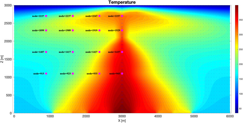
FIGURE 7. Temperature field in the Phlegraean Fields. Results of the analysis (t_fin).

FIGURE 8

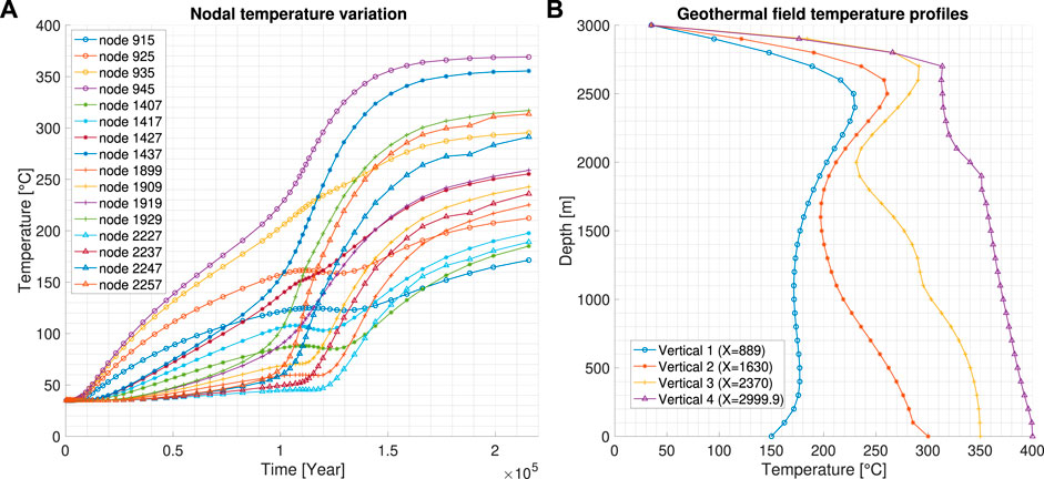
FIGURE 8. Nodal temperature variation with the time (A) and geothermal field temperature profiles (t_fin) (B).

FIGURE 9

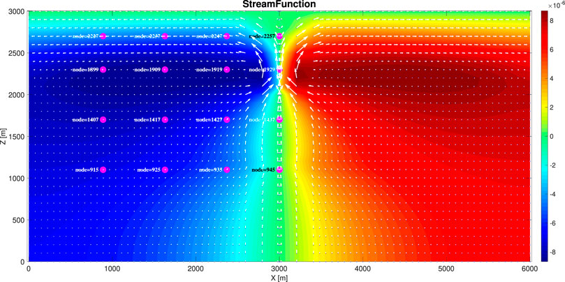
FIGURE 9. Stream function field in the Phlegraean Fields. Results of the analysis (t_fin).

4.2 Results of implementation. DBHE in service

After reaching the system’s steady-state time, t_fin, the second analysis is performed, taking into account the effects of the DBHE’s presence. The simulation is carried out up to a DBHE service time of 200 years, and a transient analysis is carried out by dividing the simulation time into 15 steps (Δ t_wb), the intervals of which are described in Supplementary Table S4; Section 4.1. The results obtained for the temperature and stream function field over the domain after 65 and 200 years of DBHE service are presented in Figures 10–13, respectively. The transient analyses shown in Figures 10, 11 demonstrate the temperature decrement around the heat extraction well. The temperature changes, after 65 years of service, affect only the area around the well (21 m in the x direction), while, after 200 years, the affected area has expanded (206.2 m in the x direction), perturbing the distribution of the temperature field in the central high part of the reservoir. Similarly, the stream function’s field variation effect is observed by comparing Figure 12 with the final analysis step in Figure 13. The latter demonstrates a change in fluid flow directionality with the reversed sign near the reservoir’s top (between depths 300 and 400 m). The fluid velocity vectors and the stream function field remain unchanged throughout the domain.

FIGURE 10

FIGURE 10. Temperature field in the Phlegraean Fields with the DBHE in service (65 years).

FIGURE 11

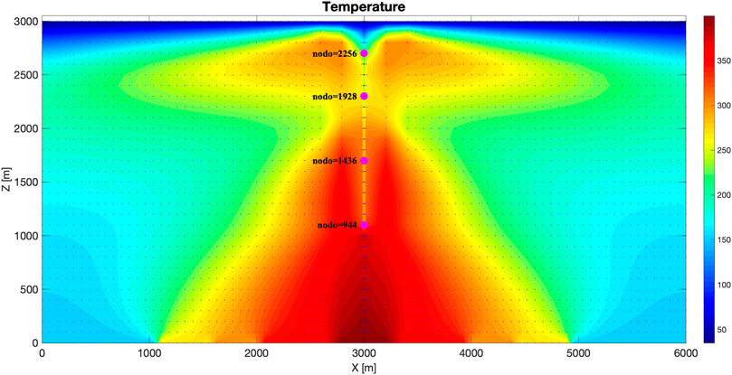
FIGURE 11. Temperature field in the Phlegraean Fields with the DBHE in service (200 years).

FIGURE 12

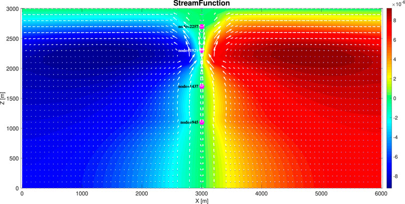
FIGURE 12. Stream function field in the Phlegraean Fields with the DBHE in service (65 years).

FIGURE 13

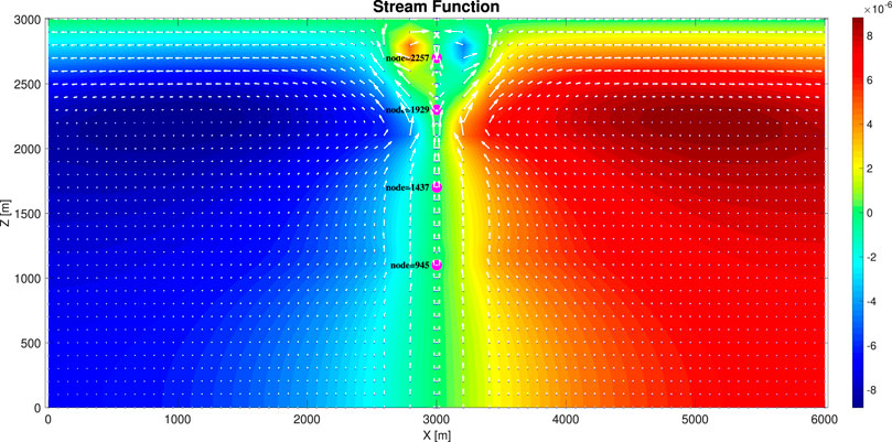
FIGURE 13. Stream function field in the Phlegraean Fields with the DBHE in service (200 years).

The temperature and stream function fields can be seen in more detail, respectively, in Figures 14, 15. Figure 14C shows the first decrease in temperature caused by the DBHE in 12 years, while this effect is not detected in the stream function field shown in Figure 15C.

FIGURE 14

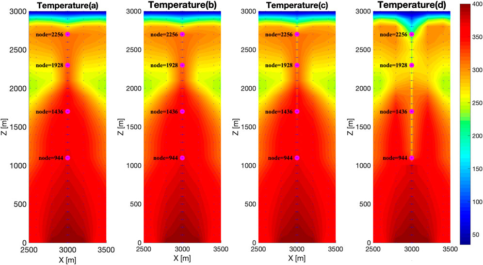
FIGURE 14. Temperature field’s time variation in the Phlegraean Fields with the DBHE in service. Results after 0.9 years (A), 3 years (B), 12 years (C), and 200 years (D).

FIGURE 15

FIGURE 15. Stream function field’s time variation in the Phlegraean Fields with the DBHE in service. Results after 0.9 years (A), 3 years (B), 12 years (C), and 200 years (D).

Finally, Figures 16A, B, respectively, show the variations of nodal temperature at four elevations (z = 1,100 m, 1,700 m, 2,300 m, and 2,700 m from the reservoir’s base) for the left and right nodes of the DBHE at a distance of 1 m in the x direction and the temperature profiles at four analysis verticals. The maximum and minimum temperatures recorded during the first and 15th analysis steps are 107.3°C at an elevation of 2,700 m (300 m depth) and 69.3°C at an elevation of 1,900 m, respectively. The values for each analysis step are reported in Supplementary Table S4 and Supplementary Table S5 of this paper.

FIGURE 16

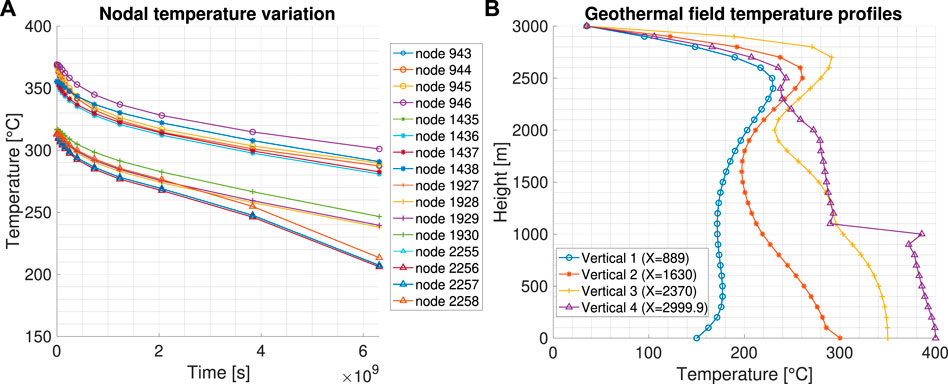
FIGURE 16. Nodal temperature time variation (A) and geothermal field temperature profile (B) with the DBHE in service (t_fin,wb = 200 years).

5 Discussion

Simulating a geothermal reservoir, specifically that of the Phlegraean Fields, and studying the effects on a DBHE’s domain is a challenging task that requires knowledge of geology, physics and applied physics, mathematics, numerical simulation methods, and computational implementation techniques. In-depth research is carried out on the geothermal reservoir, the geological parameters, and thermophysical and hydraulic characteristics found in the studies of Troise et al., 2001, Carlino et al., 2012, Costa, 2006, and Petrillo et al., 2013, as well as those gathered in this work. Through this study, we were able to identify the presence of six anisotropic layers in the vertical z direction, the potential extension of the study domain (6,000 × 3,000 m in longitude and depth), the distributed presence of magmatic sources at high temperatures, and the location of the potential fluid inlet and outlet. After obtaining the key parameters, the software was developed to define the thermal and hydraulic states of the domain in terms of temperature, stream function, and fluid directionality vectors. For this purpose, the problem was physically described using well-known equations of mass, energy, and momentum conservation laws (Todreas and Kazimi, 1990). The equations were adapted to saturated porous media as in Bejan and Kraus, 2003 and were supplemented in a two-dimensional field considering Darcy’s filtration law. The definition of the velocity components allowed us to evaluate the stream function variable (Holzbecher and Yusa, 1995) which is useful for determining the direction of the movement of water particles. The relationship governing the behavior of the DBHE is derived from Cheng et al., 2011 and Le Nian et al., 2014. The numerical method used to discretize the nonlinear partial-derivative system to solve some specific boundary conditions is the GM coupled with the second-order finite difference method. Some examples and applications of the latter can be found in Nikishkov, 2009 and Kaliakin, 2002. The DBHE could be discretized once more using the GM. The fluid density and its variations are computed nodally and are affected by parameters μ and β. These parameters were estimated using IAPWS, 2007 and Mifofski, 2013, which were then integrated into the computational code. These system closure equations play an important role in the goodness of fit of the results obtained in the transient analysis because they are strongly influenced by temperature variation. The results obtained for the studied variables and their nodal variations over the entire domain clearly show that the solution for a four-node discretization and linear polynomial shape functions is already convergent and consistent with the results of the previously mentioned scientific publications as well as the site measurements. GM, by collaborating with the pre-existing equation systems, was able to resolve the severe boundary conditions caused by the presence of the DBHE. The temperature variation at the well wall over time is consistent with the trend presented in the studies of Cheng et al., 2011 and Le Nian et al., 2014. Applying this system, the heat extraction effect of the temporal DBHE was determined by defining an optimal operating time (65 years) before which the system’s hydraulic and thermodynamic configurations did not significantly change. This methodology can be applied to all existing geothermal reservoirs. Furthermore, the implementation of the new computational code will allow future studies to investigate the weight of the constants of the porous medium, the water parameters (geo-fluid), and the composition of a hypothetic fluid (by simulating and optimizing the different thermal response parameters) contained in the DBHE (e. g., using nanoparticles). We will gradually progress to the study of three-dimensional domains, selecting the appropriate parameters to define the domain response. In addition to defining the effects of the DBHE on the domain, it is proposed to integrate a system that allows for the establishment of renewable energy production regimes that are compatible with the exploitation of the geothermal domain.

6 Conclusion

This study includes a set of numerical simulations to describe the geothermal field of the Campi Flegrei reservoir and the subsequent variation of the thermo-hydraulic parameters in the entire reservoirs while the DBHE is in service. Several conclusions can be drawn from the simulations’ results, the most important of which are as follows:

• The integration of GM and a second-order FDM discretization enables stable and convergent solutions, as in the case of DBHE discretization using GM.

• In the case without the DBHE, from the point of view of transient analysis, the reservoir reaches stationarity after an analysis time of 215,416 years which makes sense geologically, regarding the dimensions of the reservoir.

• The central part of the domain, where the magmatic thermal source is located, has the highest temperature values (Figure 7).

• The upper part of the domain is characterized by a plume-type temperature distribution that narrows between an altitude of 2,000 and 2,400 m. This effect may be a result of the change in the physical properties of the porous medium that can be deduced from the phenomena shown in Figure 9, while in the central area of the domain, the fluid directionality tends to be vertical. These phenomena, i.e., the plume-shaped distribution of temperatures and the upward flow directionality for the stream function are comparable with those presented by Petrillo et al., 2013.

• The integrated reserve–DBHE system analysis was conducted by simulating 200 years of operation. The system had not yet reached the steady state at this point, and the temperature variations occurred up to a distance (x) of 206.2 m from the well.

• At the 14th time-step of the transient simulation, corresponding to 121 years, a change in the temperature profile and stream function can be observed in the central part of the domain (see Supplementary Figures S1, S2), along with the inversion of fluid directionality maintained up to the end of the analysis.

• The maximum temperature change along the well’s wall during the 200 years was estimated to be 107.3°C. Based on this study, 65 years can be defined as a reference lifetime for sustainable geothermal energy extraction using the DBHE system.

Data availability statement

The original contributions presented in the study are included in the article/Supplementary Material, further inquiries can be directed to the corresponding author.

Author contributions

“Conceptualization, software, validation, formal analysis, resources, data curation, visualization, investigation, and funding acquisition: GS; the methodology used for implementation of GM in geothermal problems: GS and SAG; conceptualization of DBHE boundary condition: GS and CA; methodology for its implementation: AA and GS; review and editing: AA, CA, GS, and SAG; supervision: CA and SAG; writing—original draft preparation—review and editing: AA, CA, GS, and SAG. “All authors have read and agreed to the published version of the manuscript”.

Acknowledgments

We would like to thank Studio Tecnico di Ingegneria “Sepede” for providing the technological support for the development of this work (personal computer, material, and support used for writing the software and for the computational experiments). We also thank the Polytechnic University of Cartagena and the ETSIA School for providing access to the research computer platforms. Finally, we thank the DICMA department of the Sapienza University of Rome for providing valuable material and bibliographic references (articles and computers).

Conflict of interest

The authors declare that the research was conducted in the absence of any commercial or financial relationships that could be construed as a potential conflict of interest.

Publisher’s note

All claims expressed in this article are solely those of the authors and do not necessarily represent those of their affiliated organizations, or those of the publisher, the editors, and the reviewers. Any product that may be evaluated in this article, or claim that may be made by its manufacturer, is not guaranteed or endorsed by the publisher.

Supplementary material

The Supplementary Material for this article can be found online at: https://www.frontiersin.org/articles/10.3389/fenrg.2022.1000990/full#supplementary-material

References

Alimonti, C., Soldo, E., Bocchetti, D., and Berardi, D. (2018). The wellbore heat exchangers: A technical review. Renew. Energy 123, 353–381. doi:10.1016/j.renene.2018.02.055

CrossRef Full Text | Google Scholar

Bejan, A., and Kraus, A. D. (2003). Heat transfer handbook. Wiley-Interscience. Har/Cdr edition.

Google Scholar

Bertani, R. (2007). “World geothermal generation in 2007,” in Proceedings European Geothermal Congress 2007 Unterhaching, Germany, 30 May-1 June 2007.

Google Scholar

Bertani, R. (2015). Geothermal power generation in the world 2010-2014 update report. Geothermics 60, 31–43. doi:10.1016/j.geothermics.2015.11.003

CrossRef Full Text | Google Scholar

Cánovas, M., Alhama, I., García, G., Trigueros, E., and Alhama, F. (2017). Numerical simulation of density-driven flow and heat transport processes in porous media using the network method. Energies 10 (9), 1359. art. no. 1359. doi:10.3390/en10091359

CrossRef Full Text | Google Scholar

Carlino, S., Somma, R., Troise, C., and De Natale, G. (2012). The geothermal exploration of Campanian volcanoes: Historical review and future development. Renew. Sustain. Energy Rev. 16, 1004–1030. doi:10.1016/j.rser.2011.09.023

CrossRef Full Text | Google Scholar

Carlino, S., Troiano, A., Di Giuseppe, M. G., Tramelli, A., Troise, C., Somma, R., et al. (2016). Exploitation of geothermal energy in active volcanic areas: A numerical modelling applied to high temperature mofete geothermal field, at Campi Flegrei caldera (southern Italy). Renew. Energy 87, 54–66. doi:10.1016/j.renene.2015.10.007

CrossRef Full Text | Google Scholar

Cheng, W., Huang, Y., Lu, D., and Yin, H. (2011). A novel analytical transient heat-conduction time function for heat transfer in steam injection wells considering the wellbore heat capacity. Energy 36, 4080–4088. doi:10.1016/j.energy.2011.04.039

CrossRef Full Text | Google Scholar

Clauser, C. (2003). Numerical simulation of reactive flow in hot aquifers: SHEMAT and processing SHEMAT. Heidelberg-Berlin: Springer.

Google Scholar

Costa, A. (2006). Permeability–porosity relationship: A reexamination of the kozeny–carman equation based on a fractal pore-space geometry assumption. Geophys. Res. Lett. 33, L02318. doi:10.1029/2005gl025134

CrossRef Full Text | Google Scholar

Davis, A. P., and Michaelides, E. E. (2009). Geothermal power production from abandoned oil wells. Energy 34, 866–872. doi:10.1016/j.energy.2009.03.017

CrossRef Full Text | Google Scholar

Elder, J. W., Simmons, C. T., Diersch, H., Frolkoviˇc, P., Holzbecher, E., and Jo- hannsen, K. (2017). The elder problem. Rev. Fluid 2, 11. MDPI.

Google Scholar

Gupta, K. K., and Meek, J. L. (2002). Finite element multidisciplinary analysis, second edition. Springer.

Google Scholar

Holzbecher, E. O. (1998). Modelling density-driven flow in porouse media. Springer.

Google Scholar

Holzbecher, H., and Yusa, Y. (1995). Numerical experiments on free and forced convection in porous media. Int. J. Heat. Mass Tranfer 38, 2109–2115. Elsevier Science Ltd.

CrossRef Full Text | Google Scholar

IAPWS (2007). International association for the properties of water and steam, revised. Release on the IAPWS industrial formulation 1997 for the thermodynamic properties of water and steam. Lucerne, Switzerland: IAPWS.

Google Scholar

Il’in, A. M. (1969). Differencing scheme for a differential equation with a small parameter affecting the highest derivative. Math. Notes Acad. Sci. USSR 6, 596–602. doi:10.1007/bf01093706

CrossRef Full Text | Google Scholar

Kaliakin, V. (2002). Introduction to approximate solution techniques, numerical modeling and finite element methods. CRC Press, Marcel Dekker. Edition 1.

Google Scholar

Kujawa, T., Nowak, W., and Stachel, A. A. (2006). Utilization of existing deep geological wells for acquisitions of geothermal energy. Energy 31, 650–664. doi:10.1016/j.energy.2005.05.002

CrossRef Full Text | Google Scholar

Le Nian, Y., Cheng, W., Li, T., and Wang, C. (2014). Study on the effect of wellbore heat capacity on steam injection well heat loss. Appl. Therm. Eng. 70, 763–769. doi:10.1016/j.applthermaleng.2014.05.056

CrossRef Full Text | Google Scholar

Luo, Z., Wang, Y., Zhou, S., and Wu, X. (2003). Simulation and prediction of conditions for effective development of shallow geothermal energy. Appl. Therm. Eng. 91, 370–376. doi:10.1016/j.applthermaleng.2015.08.028

CrossRef Full Text | Google Scholar

MATLAB MATLAB, version R2018a (8.5.0.197613), copyright 1984-2018. Natick, Massachusetts: Math- Works, Inc.

Mifofski, M. (2013). MATLAB function, IAPWSIF97. Available at: https://mikofski.github.io/IAPWSIF97/Copyright(c).

Google Scholar

Nalla, G., Shook, G. M., Mines, G. L., and Bloomfield, K. K. (2005). Parametric sensitivity study of operating and design variables in wellbore heat exchangers. Geothermics 34, 330–346. doi:10.1016/j.geothermics.2005.02.001

CrossRef Full Text | Google Scholar

Nikishkov, G. (2009). Programming finite elements in java. Springer.

Google Scholar

Noorollahi, Y., Pourarshad, M., Jalilinasrabady, S., and Yousefi, H. (2015). Numerical simulation of power production from abandoned oil wells in Ahwaz oil field in southern Iran. Geothermics 55, 16–23. doi:10.1016/j.geothermics.2015.01.008

CrossRef Full Text | Google Scholar

Petrillo, Z., Chiodini, G., Mangiacapra, A., Caliroa, S., Capuanob, P., Russo, G., et al. (2013). Defining a 3D physical model for the hydrothermal circulation at Campi Flegrei caldera (Italy). J. Volcanol. Geotherm. Res. 264, 172–182. doi:10.1016/j.jvolgeores.2013.08.008

CrossRef Full Text | Google Scholar

Ramey, H. J. (1962). Wellbore heat transmission. J. Petroleum Technol. 14, 427–435. doi:10.2118/96-pa

CrossRef Full Text | Google Scholar

Renaud, T., Verdin, P., and Falcone, G. (2019). Numerical simulation of a deep borehole heat exchanger in the krafla geothermal system. Int. J. Heat Mass Transf. 143, 118496. doi:10.1016/j.ijheatmasstransfer.2019.118496

CrossRef Full Text | Google Scholar

Tang, H., Xu, B., Hasan, A. R., Sun, Z., and Killough, J. (2019). Modeling wellbore heat exchangers: Fully numerical to fully analytical solutions. Renew. Energy 133, 1124–1135. doi:10.1016/j.renene.2018.10.094

CrossRef Full Text | Google Scholar

Templeton, J. D., Ghoreishi-Madiseh, S. A., Hassani, F., and Al-Khawaja, M. J. (2014). Abandoned petroleum wells as sustainable sources of geothermal energy. Energy 70, 366–373. doi:10.1016/j.energy.2014.04.006

CrossRef Full Text | Google Scholar

Todreas, N., and Kazimi, M. (1990). Nuclear systems 1: Thermal hydraulic fundamentals. New York: CRC press.

Google Scholar

Troise, C., Castagnolo, D., Peluso, F., Gaeta, F. S., Mastrolorenzo, G., De Natale, G., et al. (2001). 2D mechanical thermalfluid dynamical model for geothermal systems at calderas: An application to Campi Flegrei, Italy. J. Vulcanology Geotherm. Res. 109, 1–12. doi:10.1016/S0377-0273(00)00301-2

CrossRef Full Text | Google Scholar

Westaway, R. (2018). Deep geothermal single well heat production: Critical appraisal under UK conditions. Quart. J. Engin. Geol. Hydrogeol. 51, 424–449. doi:10.1144/qjegh2017-029

CrossRef Full Text | Google Scholar

Yusa, Y. (1983). Numerical experiment of groundwater motion under geothermal condition.-vying between potential flow and thermal convective flow. J. Geotherm. Res. Soc. Jpn. 5 (1), 23–38. doi:10.11367/grsj1979.5.23

CrossRef Full Text | Google Scholar

Nomenclature

(ρ c) Heat capacity (J m⁻¹K⁻¹)

∂Q/∂z Deep borehole heat exchanger heat loser or rate of heat flow over dz (W m⁻¹)

A_wb Area of the DBHE (m²)

B.C. Boundary condition

c Specific heat (J kg⁻¹K⁻¹)

C₁ Euler’s constant 0.5772 [—]

DBHE Deep-borehole heat exchangers

f(t)* Transient heat-conduction time function [—]

FDM Finite difference method

FEM Finite element method

GM Galerkin method

H Height of reservoir (m)

I.C. Initial condition

K Hydraulic permeability (m²)

k Thermal conductivity (W m⁻¹K⁻¹)

P Pressure (MPa)

Q Heat flux (W m⁻²)

r Radius of the well (m)

Subscript s, solid or soil part, f, fluid part, m, porous medium, ei, formation, wb, wellbore n, node, and e, element

T Temperature parameter (°C)

t Time [s]

t₀ Initial time [s]

T_ei Temperature in the formation node (°C)

t_fin Final time [s]

α Thermal diffusivity (m²s⁻¹)

T_wb Temperature in the deep borehole heat exchanger’s wall (°C)

U Length of reservoir (m)

v_x Velocity horizontal component (m s⁻¹)

v_z Velocity vertical component (m s⁻¹)

x Horizontal distance (m)

z Vertical distance (m)

β Expansion coefficient (°C⁻¹)

Γ Boundary condition position on the body line

Δt Time step of analysis [s]

μ Dynamic viscosity of water (kg m⁻¹ s⁻¹)

ρ Density (kg m⁻³)

ρ₀ Density of water at the reference temperature (kg m⁻³)

σ Heat capacity ratio [—]

τ_d Dimensionless time (s)

φ Porosity of soil [—]

χ The mathematical system

ψ Stream-function flow parameter (m² s⁻¹)

Ω Computational domain