Extreme learning Kalman filter for short-term wind speed prediction

1 Introduction

To support environmental sustainability, wind energy is the best green energy source to replace high-carbon power generation. The use of wind power has increased dramatically, particularly in the past decade. It is challenging to control wind turbines and implement optimal wind farm operations for reliable wind power supplementation due to the stochastic nature of wind speed (Evans and Lio, 2022). It is crucial to obtain precise wind speed predictions for optimal control of wind turbines, using methods such as models of predictive control in stabilizing wind turbines (Hur and Leithead, 2022), to ensure stable supply of wind power. Predicting wind speed, especially in the short-term, is critical for improving power generation efficiency and extending the life span of a wind turbine (Bossanyi, 2003; Lio et al., 2017; Liew et al., 2022).

The existing methods for wind speed prediction in the short term represent two different classes. The first class includes physical model-based methods (Cassolaa and Burlando, 2012; Xu et al., 2020; Chen et al., 2021; Li et al., 2022). One physical model-based method is the numerical weather prediction method, in which predictions are based on physical models that include parameters characterizing the properties of the weather, such as atmospheric pressure, surface roughness, temperature, and many others (Lynch, 2008; Chen et al., 2021). However, the performance of the numerical weather prediction method deteriorates dramatically when the uncertainty of weather conditions is high. To address the uncertain nature of wind speed, statistical modeling has become more and more popular compared to models of the physical mechanism of wind speed. In the statistical approach, statistical methods are applied to model the temporal causality of wind speed (Shen et al., 2021; Ouyang et al., 2017). Currently, wind speed prediction often uses time series models or artificial neural network (ANN) models (Giorgi et al., 2011). Among time series model-based methods, autoregressive moving average (ARMA) models, with variants such as simplified autoregressive (AR) models and others, have been well-applied in forecasting wind speed sequence (Prema and Rao, 2015; Torres et al., 2005; Hanoon et al., 2022). However, the ARMA class methods need to increase model order to model causality in a time series, especially considering the stochastic variations of wind speed. Moreover, ARMA models are essentially linear models, which are not able to capture nonlinear features of the causality of wind speed. Therefore, ANNs are used to describe the nonlinear features of temporal causality in wind speed (Başaran and Filik, 2017; Kadhem et al., 2017; Malik et al., 2022). Although ANNs can handle the nonlinearity in wind speed dynamics, they cannot independently capture the dynamical nature of wind speed time series; therefore, a high-order model is necessary, which increases the complexity of the model.

State-space models are naturally suitable for describing the temporal causality of a dynamical system (Shen et al., 2020). Kalman filters can be used to identify the state-space models and infer the hidden state variables (Kitagawa, 1996; Kitagawa, 1987). Kalman filtering has been widely used in estimation problems, such as battery capacity estimation (Plett, 2004a; Plett, 2004b; Plett, 2004c; Plett, 2006a; Plett, 2006b). For nonlinear models, use of a sigma-point Kalman filter (SPKF) is an effective way to conduct the state estimation (Plett, 2006a; Plett, 2006b). However, accuracy of the SPKF relies on the goodness-of-fit of the model. Therefore, in this article, we propose the Extreme Learning Kalman Filter (ELKF), a novel method that combines SPKF and ANN to give accurate short-term predictions of wind speed. Our data indicate that the state-space model for wind speed can be obtained using noisy measurements of wind speed. With an ANN-based state-space model for dynamics of wind speed, we conduct SPKF modeling to obtain estimates of current wind speed, then use the estimation and an ANN-based state equation to further predict wind speed. The effectiveness of the proposed ELKF model has been validated using an experimental data set.

This article is organized into four sections. Section 2 includes a formal description of the problem. In Section 3, the proposed algorithm is presented after a brief introduction to the Extreme Learning Machine (ELM) based training algorithm for ANNs and SPKF. The results of experimental data-based validations are presented in Section 4, and the study conclusion appears in Section 5.

2 Problem formulation

Let t = 0, 1, 2, … define the discrete time index. Let $s_t\in \mathbb{R}$ be the wind speed at t. The following assumption holds throughout this article.

Assumption 1. The stochastic process s_t is a Markov process. Namely, the following holds.

$\begin{array}{ll}\hfill & \mathbf{P}\mathbf{r}\left\{s_{t+1}=S^{\prime }|s_t=S,s_{t-1}=S_{t-1},\dots ,s_0=S_0\right\}\hfill \\ \hfill & \hfill =\mathbf{P}\mathbf{r}\left\{s_{t+1}=S^{\prime }|s_t=S\right\}.\end{array}(1)$

Due to Assumption 1, we can use the state-space equation to describe the dynamical evolution of s_t, which is written by

$s_{t+1}=f_{\text{ws}}\left(s_t,{\omega }_t\right),(2)$

where ${\omega }_t\in \mathbb{R}$ is a random variable for system noise, and $f_{\text{ws}}:\mathbb{R}\times \mathbb{R}\to \mathbb{R}$ is an unknown nonlinear function that describes the causality relationship between s_t and s_t+1. The measurement of wind speed z_t is perturbed by s_t due to the existence of measurement noise ν_t. The observation function is thus written by

$z_t=s_t+{\nu }_t.(3)$

We hold the following assumptions regarding ω_t and ν_t.

Assumption 2. The system noise ω_t and measurement noise ν_t are both identically independently distributed Gaussian noises.The problem that needs to be addressed is summarized as follows.Problem 1. With data set ${\mathcal{Z}}_t=\{z_0,\dots ,z_t\}$, this study aims to predict ${\widehat{s}}_{t^{\prime }}$ of s_t′ for a t′ > t. The prediction ${\widehat{s}}_{t^{\prime }}$ is expected to satisfy

$\mathbb{E}\left\{{\widehat{s}}_{t^{\prime }}-s_{t^{\prime }}\right\}=0,(4)$

and

$\mathbb{E}\left\{{\left({\widehat{s}}_{t^{\prime }}-s_{t^{\prime }}\right)}^2\right\}=\mathbb{E}\left\{{\nu }_t^2\right\}.(5)$

To achieve the task, the following two sub-problems need to be addressed:

• construction of the approximate model ${\widehat{f}}_{\text{ws}}(\cdot )$ of f_ws(⋅);

• design of filtering and prediction algorithms to estimate ${\widehat{s}}_t$ and prediction of ${\widehat{s}}_{t^{\prime }}$.

3 Proposed method

3.1 ELM for training ANNs

ELM is an effective algorithm for training single-layer ANNs. Single-layer ANNs can be well trained to approximate standard multilayer ANNs. In a single-layer ANN, there are nonlinear activation functions as hidden nodes. For example, there are N samples (u_i, o_i), where $o_i={[o_{i,1},\dots ,o_{i,m}]}^{\mathrm{T}}\in {\mathbb{R}}^m$ represents the output variable and $u_i={[u_{i,1},\dots ,u_{i,n}]}^{\mathrm{T}}\in {\mathbb{R}}^n$ is the input. A single-layer ANN denoted by h(u) with S activation function φ(⋅) describes the input-to-output causality by

${\widehat{o}}_i=h\left(u_i\right)⩵\sum _{j=1}^S{\beta }_j\phi \left({\omega }_j^{\mathrm{T}}{u}_i+b_j\right),i=1,\dots ,N(6)$

where ${\omega }_j={[{\omega }_{j,1},\dots ,{\omega }_{j,n}]}^{\mathrm{T}}$ and ${\beta }_j={[{\beta }_{j,1},\dots ,{\beta }_{j,m}]}^{\mathrm{T}}$ are vectors, and b_j is a constant scalar in the jth node. If we consider the relationship between o and u, it is described by o = h(u) and is nonlinear, as shown in the left part of Figure 1. On the other hand, if we consider o and φ(⋅), the causality becomes linear after activation function mapping, as shown in the right part of Figure 1.

FIGURE 1

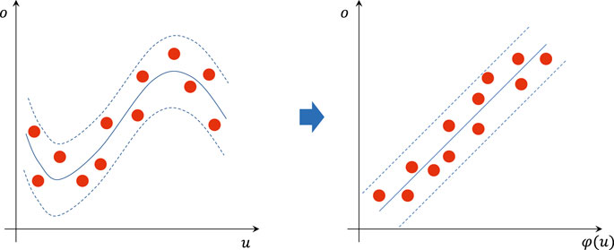
FIGURE 1. Essentials of the ELM algorithm: activation function mapping.

A single-layer ANN with S activation function φ(⋅) can approximate these N samples in the sense of zero means written by

$\sum _{i=1}^N{e}_i=\sum _{i=1}^N\left(o_i-{\widehat{o}}_i\right)=0,(7)$

then, by the theoretical result in Huang (2003), ∃S ≤ N, b_j, ω_j, β_j such that

$o_i=\sum _{j=1}^S{\beta }_j\phi \left({\omega }_j^{\mathrm{T}}{u}_i+b_j\right),i=1,\dots ,N.(8)$

where the activation function adopts the same function denoted by φ(⋅). More generally, by defining

$H=\left[\begin{array}{ccc}\hfill \phi \left({\omega }_1^{\mathrm{T}}{u}_1+b_1\right)\hfill & \hfill \dots \hfill & \hfill \phi \left({\omega }_{\bar{N}}^{\mathrm{T}}{u}_1+b_{\bar{N}}\right)\hfill \\ \hfill ⋮\hfill & \hfill \dots \hfill & \hfill ⋮\hfill \\ \hfill \phi \left({\omega }_{\bar{N}}^{\mathrm{T}}{u}_N+b_1\right)\hfill & \hfill \dots \hfill & \hfill \phi \left({\omega }_{\bar{N}}^{\mathrm{T}}{u}_N+b_{\bar{N}}\right)\hfill \end{array}\right],(9)$

$\beta =\left[\begin{array}{c}\hfill {\beta }_1^{\mathrm{T}}\hfill \\ \hfill ⋮\hfill \\ \hfill {\beta }_{\bar{N}}^{\mathrm{T}}\hfill \end{array}\right],(10)$

and

$O=\left[\begin{array}{c}\hfill o_1^{\mathrm{T}}\hfill \\ \hfill ⋮\hfill \\ \hfill o_{\bar{N}}^{\mathrm{T}}\hfill \end{array}\right],(11)$

the above equation is equivalent to

$O=H\beta .(12)$

We call H the output matrix of the hidden layer or the hidden layer output matrix. The ith column of H represents the ith hidden node output computed from the inputs u₁, u₂, … , u_N. Generally, the values of $\beta ,{\omega }_1,\dots ,{\omega }_{\bar{N}},b_1,\dots ,b_{\bar{N}}$ can be trained by using a gradient descent algorithm. However, the ELM algorithm proposed in Huang (2003) provides a simpler and more efficient way to obtain good estimations of $\beta ,{\omega }_1,\dots ,{\omega }_{\bar{N}},b_1,\dots ,b_{\bar{N}}$ in the sense of zero means.

Let U = [u₁, u₂, … , u_N] be the input matrix and O be the output matrix. The ELM algorithm for training single-layer ANNs is summarized in Algorithm 1. Note that H^M represents the generalized inverse of H, called the Moore-Penrose generalized inverse, which is defined in Rao and Mitra (1972) and is calculated as

$H^M={\left(H^{\mathrm{T}}H\right)}^{-1}{H}^{\mathrm{T}}.(13)$

Thus, we calculate the estimation of β by

$\beta ={\left(H^{\mathrm{T}}H\right)}^{-1}{H}^{\mathrm{T}}O.(14)$

The effectiveness of Algorithm 1 is theoretically proven in Tamura and Tateishi (1997) when we assume that H is invertible, φ(⋅) is infinitely differentiable, and $‖H\beta -O‖=0$.

Algorithm 1. Original ELM for single-layer ANNs

Input: U, O, S

Output: b_j, ω_j, β, j = 1, 2, … , S

Step 1: Generate b_j and ω_j, $j=1,\dots ,\bar{N}$ by random algorithm (uniform distribution);

Step 2: Compute H;

Step 3: Compute β = H^MO

A sequential version can also be derived by way of the recursive least squares (RLS) algorithm (Chong and Zak, 2001), which is summarized as

3.2 Brief introduction to SPKF

SPKF is a generalized Kalman filter for estimating the state of nonlinear dynamical systems described by

$x_{t+1}=f\left(x_t,w_t\right),(15)$

$y_t=g\left(x_t,v_t\right),(16)$

where $x_t\in {\mathbb{R}}^{n_x}$ denotes the state variable, $y_t\in {\mathbb{R}}^m$ is the observation, and w_t, v_t are noises. Instead of using Taylor-series expansion-based approximations of the covariance matrices of the state and output as in the extended Kalman filter (EKF) (Plett, 2004a; Plett, 2004b; Plett, 2004c), several functions are evaluated to calculate the approximations of the covariance matrices. SPKF does not require the differentiability of the original functions in state-space models and can achieve better approximations of covariance matrices, which improves state estimation accuracy. Additionally, in SPKF, the derivatives of the functions in the state-space models are not required, which also reduces the computational complexity of implementing SPKF.

In SPKF, several sigma points are selected to be the input of the nonlinear function. Note that the mean and covariance of the sigma points can be weighted to the values that are equal to the those of the a priori state estimation. These points are directed to a set of points output by the nonlinear function, which can be used to obtain the approximate mean and covariance of the a posteriori estimated state. In the state estimation problem for a system described by (Eqs 15, 16), the required number of sigma points is p + 1 = 2n_x + 1. The generated set is defined by

${\mathcal{X}}_{t,i}=\left\{{\bar{x}}_{t,i},{\bar{x}}_{t,i}+\gamma \sqrt{{\mathrm{\Sigma }}_{x_t}},{\bar{x}}_{t,i}-\gamma \sqrt{{\mathrm{\Sigma }}_{x_t}}\right\},i=0,\dots ,p,(17)$

where the matrix square root $B=\sqrt{A}$ is the result of $A=B{B}^{\mathrm{T}}$, ${\bar{x}}_t$ is the mean of x_t, and ${\mathrm{\Sigma }}_{x_t}$ is the covariance of x_t. It can find a specific set of {γ, α^(m), α^(c)} such that the weighted mean and covariance of ${\mathcal{X}}_{t,i}$ equal the original mean and covariance of x_t, which are written by

$\bar{x}=\sum _{i=0}^p{\alpha }_i^{\left(m\right)}{\mathcal{X}}_{t,i},(18)$

${\mathrm{\Sigma }}_{x_t}=\sum _{i=0}^p{\alpha }_i^{\left(c\right)}\left({\mathcal{X}}_{t,i}-\bar{x}\right){\left({\mathcal{X}}_{t,i}-\bar{x}\right)}^{\mathrm{T}}.(19)$

Note that ${\sum }_{i=0}^p{\alpha }_i^{(m)}=1$ and ${\sum }_{i=0}^p{\alpha }_i^{(c)}=1$.

Let $x_t^a={[{(x_t)}^{\mathrm{T}},w_t,v_t]}^{\mathrm{T}}$ be an augmented random variable. With $x_t^a$, we implemented SPKF as follows.

1) Update of the a priori state estimation. First, there is augmentation of a posteriori state estimation of the last time step,

${\widehat{x}}_{t-1}^{a,+}={\left[{\left({\widehat{x}}_t^{+}\right)}^{\mathrm{T}},{\bar{w}}_t,{\bar{v}}_t\right]}^{\mathrm{T}},(20)$

and then augmentation of a posteriori covariance estimation,

${\mathrm{\Sigma }}_{x_{t-1}}^{a,+}=\text{diag}\left({\mathrm{\Sigma }}_{x_{t-1}}^{+},{\mathrm{\Sigma }}_w,{\mathrm{\Sigma }}_v\right).(21)$

Based on (Eqs 20, 21), we can generate p + 1 sigma points

$\begin{array}{ll}\hfill & {\mathcal{X}}_{t-1,i}^{a,+}=\left\{{\bar{x}}_{t-1,i}^{a,+},{\bar{x}}_{t-1,i}^{a,+}+\gamma \sqrt{{\mathrm{\Sigma }}_{x_{t-1}}^{a,+}},{\bar{x}}_{t-1,i}^{a,+}-\gamma \sqrt{{\mathrm{\Sigma }}_{x_{t-1}}^{a,+}}\right\}\hfill \\ \hfill & ,i=0,\dots ,p.\hfill \end{array}(22)$

In ${\mathcal{X}}_{t-1,i}^{a,+}$, we extract the state portion ${\mathcal{X}}_{t-1,i}^{x,+}$ and the measurement noise portion ${\mathcal{X}}_{t-1,i}^{w,+}$ to evaluate the state equation to calculate the a priori sigma points ${\mathcal{X}}_{t,i}^{x,-}$ for time step t, which is written as

${\mathcal{X}}_{t,i}^{x,-}=f\left({\mathcal{X}}_{t-1,i}^{a,+},{\mathcal{X}}_{t-1,i}^{w,+}\right).(23)$

The a priori state estimation at time step t is calculated as

$\begin{array}{ll}\hfill {\widehat{x}}_t^{-}& =\mathbb{E}\left\{f\left(x_{t-1},w_{t-1}\right)|{\mathbb{Y}}_{t-1}\right\},\hfill \\ \hfill & \approx \sum _{i=0}^p{\alpha }_i^{\left(m\right)}f\left({\mathcal{X}}_{t-1,i}^{a,+},{\mathcal{X}}_{t-1,i}^{w,+}\right)=\sum _{i=0}^p{\alpha }_i^{\left(m\right)}{\mathcal{X}}_{t,i}^{x,-}.\hfill \end{array}(24)$

2) Update of the error covariance. The a priori covariance estimation is obtained from the a priori sigma points ${\mathcal{X}}_{t,i}^{x,-},i=\mathrm{0,1},\dots ,p$. That is

${\mathrm{\Sigma }}_{x_t}^{-}=\sum _{i=0}^p{\alpha }_i^{\left(c\right)}\left({\mathcal{X}}_{t,i}^{x,-}-{\widehat{x}}_t^{-}\right){\left({\mathcal{X}}_{t,i}^{x,-}-{\widehat{x}}_t^{-}\right)}^{\mathrm{T}}.(25)$

3) Estimation of the system output. The estimation of system output is computed from sigma points by using the observation equation. First, we calculate the estimated points

${\mathcal{Y}}_{t,i}=g\left({\mathcal{X}}_{t,i}^{x,-},{\mathcal{X}}_{t,i}^{v,-}\right).(26)$

The output prediction is then given by

$\begin{array}{ll}\hfill {\widehat{y}}_t& =\mathbb{E}\left\{h\left(x_t,v_t\right)|{\mathbb{Y}}_{t-1}\right\},\hfill \\ \hfill & \approx \sum _i^{\left(m\right)}h\left({\mathcal{X}}_{t,i}^{x,-},{\mathcal{X}}_{t,i}^{v,-}\right)=\sum _{i=0}^p{\alpha }_i^{\left(m\right)}{\mathcal{Y}}_{t,i}.\hfill \end{array}(27)$

4) Determination of the estimated gain matrix. To calculate the estimated gain matrix, the required covariance matrices are first be computed by

${\mathrm{\Sigma }}_{y_t}={\mathrm{\Sigma }}_{i=0}^p{\alpha }_i^{\left(c\right)}\left({\mathcal{Y}}_{t,i}-{\widehat{y}}_t\right){\left({\mathcal{Y}}_{t,i}-{\widehat{y}}_t\right)}^{\mathrm{T}},(28)$

${\mathrm{\Sigma }}_{x_t,y_t}^{-}={\mathrm{\Sigma }}_{i=0}^p{\alpha }_i^{\left(c\right)}\left({\mathcal{X}}_{t,i}^{x,-}-{\widehat{x}}_t^{-}\right){\left({\mathcal{Y}}_{t,i}-{\widehat{y}}_t\right)}^{\mathrm{T}}.(29)$

Then, we simply compute $L_t={\mathrm{\Sigma }}_{x_t,y_t}^{-}{\mathrm{\Sigma }}_{y_t}^{-}$.

5) Update of the a posteriori state estimation. The a posteriori state estimation is

${\widehat{x}}_t^{+}={\widehat{x}}_t^{-}+L_t\left(y_t-{\widehat{y}}_t\right).(30)$

6) Computation of error covariance. We compute the covariance matrix of error by

${\mathrm{\Sigma }}_{x_t}^{+}={\mathrm{\Sigma }}_{x_t}^{-}-L_t{\mathrm{\Sigma }}_{{\widehat{y}}_t}{L}_t^{\mathrm{T}}.(31)$

3.3 Proposed algorithm

The framework of the ELKF method for predicting wind speed is illustrated in Figure 2 and the proposed algorithm is summarized in Algorithm 2.

Algorithm 2. Algorithm for the proposed ELKF method.

TRAIN$({\widehat{f}}_{\text{ws}}(\cdot ))$

 $\mathbf{\text{Measure the data set}}{\mathcal{Z}}_T$

 chooseactivationfunction ϕ(⋅)

 setthenumberofactivationfunctions S

 Implement Algorithm 1 and obtain ${\widehat{f}}_{\text{ws}}(\cdot )$

 return ${\widehat{f}}_{\text{ws}}(\cdot )$

PREDICT$({\widehat{s}}_{t^{\prime }})$

 Update ${\widehat{f}}_{\text{ws}}(\cdot )$ with new data z_t via Algorithm 2

 Implement SPKF to obtain ${\widehat{s}}_t^{+}$ based on ${\widehat{f}}_{\text{ws}}(\cdot )$

 Calculate ${\widehat{s}}_{t^{\prime }}^{-}$ based on ${\widehat{f}}_{\text{ws}}(\cdot )$ and ${\widehat{s}}_t^{+}$

 return ${\widehat{s}}_{t^{\prime }}^{-}$

FIGURE 2

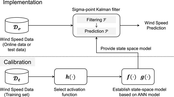
FIGURE 2. Framework of the ELKF method for predicting wind speed.

In the training step, the history data set ${\mathcal{Z}}_T$ is used to train the approximate model ${\widehat{f}}_{\text{ws}}(\cdot )$ of f_ws(⋅). The model is written by

$z_t={\widehat{f}}_{\text{ws}}\left(z_{t-1}\right)=\sum _{j=1}^S{\beta }_j\phi \left({\omega }_j^{\mathrm{T}}{z}_{t-1}+b_j\right),t=1,\dots ,T.(32)$

By implementing Algorithm 1, we obtain ${\beta }_j,{\omega }_j^{\mathrm{T}},b_j$ for j = 1, … , S with data set ${\mathcal{Z}}_T$. Here, z_t is used instead of s_t. The following theorem states that we can use z_t to get ${\widehat{f}}_{\text{ws}}(\cdot )$ in the sense of mean value.

Theorem 1. Assume that Assumption 2 holds. Then, if

$\mathbb{E}\left\{z_t\right\}=\mathbb{E}\left\{{\widehat{f}}_{\text{ws}}\left(z_{t-1}\right)\right\}t=1,\dots ,T,(35)$

then the following equation holds

$\mathbb{E}\left\{s_t\right\}=\mathbb{E}\left\{{\widehat{f}}_{\text{ws}}\left(s_{t-1}\right)\right\}t=1,\dots ,T.(36)$

Proof. Since Assumption 2 holds. We have

$\begin{array}{ll}\hfill \mathbb{E}\left\{z_t\right\}& =\mathbb{E}\left\{s_t+{\nu }_t\right\},\hfill \\ \hfill & =\mathbb{E}\left\{s_t\right\}+\mathbb{E}\left\{{\nu }_t\right\},\hfill \\ \hfill & =\mathbb{E}\left\{s_t\right\}.\hfill \end{array}(37)$

On the other hand,

$\begin{array}{ll}\hfill \mathbb{E}\left\{{\widehat{f}}_{\text{ws}}\left(z_{t-1}\right)\right\}& ={\widehat{f}}_{\text{ws}}\left(\mathbb{E}\left\{z_{t-1}\right\}\right),\hfill \\ \hfill & ={\widehat{f}}_{\text{ws}}\left(\mathbb{E}\left\{s_{t-1}+{\nu }_{t-1}\right\}\right),\hfill \\ \hfill & ={\widehat{f}}_{\text{ws}}\left(\mathbb{E}\left\{s_{t-1}\right\}+\mathbb{E}\left\{{\nu }_{t-1}\right\}\right),\hfill \\ \hfill & ={\widehat{f}}_{\text{ws}}\left(\mathbb{E}\left\{s_{t-1}\right\}\right),\hfill \\ \hfill & =\mathbb{E}\left\{{\widehat{f}}_{\text{ws}}\left(s_{t-1}\right)\right..\hfill \end{array}(38)$

Thus, (36) holds.

In the implementation step, the estimated model ${\widehat{f}}_{\text{ws}}(\cdot )$ is updated with online data z_t by Algorithm 3. Then, with ${\widehat{f}}_{\text{ws}}(\cdot )$, SPKF is implemented to obtain the a posteriori state estimation ${\widehat{s}}_t^{+}$. With ${\widehat{s}}_t^{+}$, the prediction at time step t′ > t is calculated by iteratively implementing the following equation

${\widehat{s}}_{t_j+1}^{-}={\widehat{f}}_{\text{ws}}\left({\widehat{s}}_{t_j}^{-}\right),j=0,\dots ,\left(t^{\prime }-t\right),(39)$

where t₀ = t.

Algorithm 3. Sequential ELM algorithm

Step 1: Initialize β by β₀ which is obtained from historical data by Algorithm 1

Step 2: Compute h_t+1 based on new measurement (u_t+1, o_t+1) according to Eq. 9, k = 0, 1, 2, … , i, …

Step 3: Update β_t+1 by

${\beta }_{t+1}={\beta }_t+M_{t+1}{h}_{t+1}\left(o_{t+1}^{\mathrm{T}}-h_{t+1}^{\mathrm{T}}{\beta }_t\right)(33)$

where M_t+1 is computed by

$M_{t+1}=M_t-\frac{M_k{h}_{t+1}{h}_{t+1}^{\mathrm{T}}{M}_t}{1+h_{t+1}^{\mathrm{T}}{M}_t{h}_{t+1}}.(34)$

Step 4: Set t = t + 1

4 Validation

4.1 Methods for comparison and the wind speed data set

Figure 3 illustrates the data set used in validation. The data sampling time is 10 min. A total of 61,858 data points were collected from a large wind farm located in Jiugongshan, Hubei, China within 12 consecutive days. The wind speed profiles exhibit similarity in time scale. We used the data from Day 1 to Day 10 for training the model and the rest of the data as the test set.

FIGURE 3

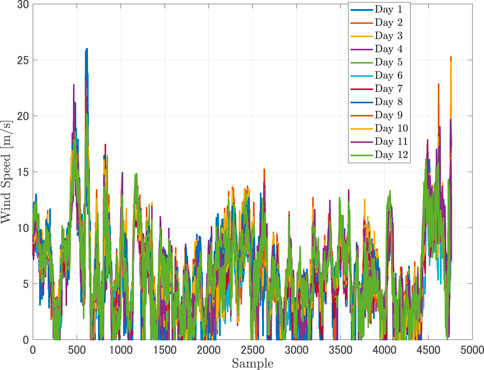
FIGURE 3. Data set for validation.

We compared the proposed ELKF method with the AR model and the ANN model. The ANN model is as described in Section 3. For n-step-ahead prediction, the addressed output is z_t′ and the input is ${[z_{t^{\prime }-n},z_{t^{\prime }-n-1},\dots ,z_{t^{\prime }-n-p+1}]}^{\mathrm{T}}$. Here, p is the order. The regular AR model is expressed by

$z_{t^{\prime }}={\alpha }_1{z}_{t^{\prime }-n}+\cdots +{\alpha }_p{z}_{t^{\prime }-n-p+1},(40)$

where α₁, … , α_p are regression coefficients.

4.2 Results and discussion

Figure 4 and Figure 5 show plots of the results of predictions (one-step and five-step) for 200 samples using the AR model, ANN model, and ELKF method. The proposed ELKF method exhibits better performance compared to the AR model and the ANN model for both prediction horizons, since the predictions given by the AR and ANN models deviate significantly from the actual values. The predictions given by the proposed ELKF method are close to the actual values. Additionally, histograms of prediction residuals for both prediction horizons are shown in Figure 6. The proposed method has the predicted residuals concentrated to zero with relatively small fluctuation. The traditional methods result in residuals with larger variation. Therefore, our data suggest that the proposed ELKF method provides more reliable predictions.

FIGURE 4

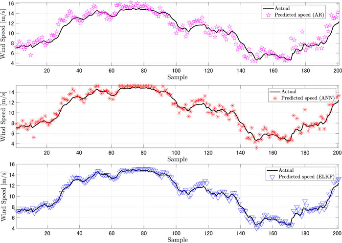
FIGURE 4. Results of wind speed prediction (predictive horizon: one-step): AR, ANN, and ELKF.

FIGURE 5

FIGURE 5. Results of wind speed prediction (predictive horizon: five-step): AR, ANN, and ELKF.

FIGURE 6

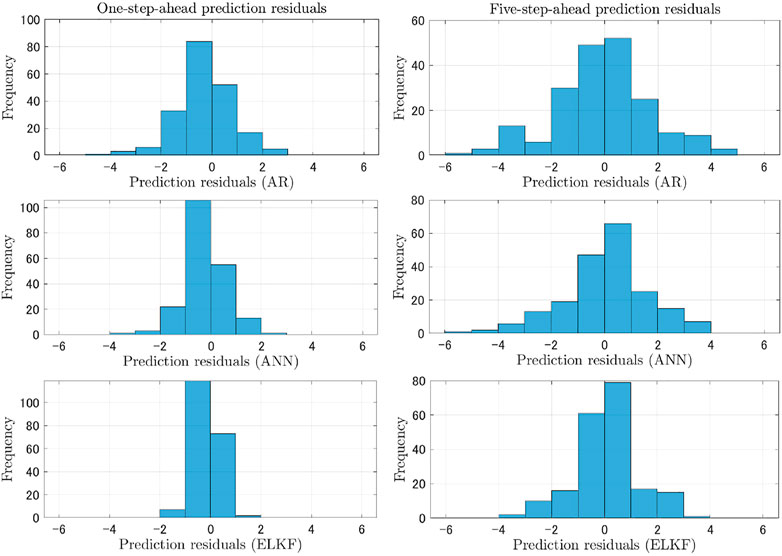
FIGURE 6. Probabilistic histograms of prediction residuals of AR, ANN, and ELKF.

Furthermore, the correlations between the predictions and the actual values of the samples in Figures 4 and 5 are plotted in Figure 7 and Figure 8, respectively. Compared to the AR and ANN models, the predictions given by the proposed ELKF method show smaller deviations and strong correlations between the actual values and predictions.

FIGURE 7

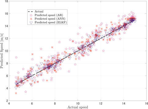
FIGURE 7. Correlation plots of one-step-ahead predictions versus actual values: AR, ANN, and ELKF.

FIGURE 8

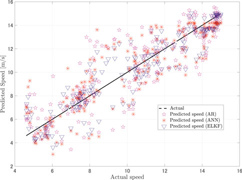
FIGURE 8. Correlation plots of five-steps-ahead predictions versus actual values: AR, ANN, and ELKF.

The results of root mean square error (RMSE) of performance of different methods from analysis of the full test data are summarized in Table 1. The results of the mean absolute error (MAE) calculation based on the performance of different methods are summarized in Table 2. RMSE is calculated by

$\text{RMSE}=\sqrt{\frac{1}{T}\sum _{t=1}^T{\left(y_t-{\widehat{y}}_t\right)}^2}.(41)$

MAE is calculated by

$\text{MAE}=\frac{1}{T}\sum _{t=1}^T|y_t-{\widehat{y}}_t|.(42)$

Our data indicate that the proposed ELKF method outperforms the AR and ANN models in different predictive horizons. The prediction performance of all methods degrades when the prediction horizon increases because the stochasticity become stronger when the prediction horizon becomes longer.

TABLE 1

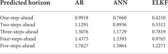
TABLE 1. Comparison of RMSE values (m/s) associated with values predicted by AR, ANN, and ELKF.

TABLE 2

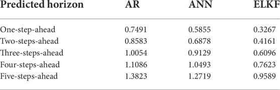
TABLE 2. Comparison of MAE values (m/s) associated with values predicted by AR, ANN, and ELKF.

The reason that the AR model does not give good predictions is that it is a linear time-series model that does not account for dynamic state update in wind speed sequence. The ANN adopts a nonlinear model and is able to depict the nonlinear feature of causality in wind speed sequence. However, the feature of dynamic state update remains unresolved. The proposed ELKF method adopts an ANN model in the dynamic system to address the nonlinear issue and uses SPKF to resolve the feature of dynamic state update. Therefore, the proposed ELKF method provides better performance in wind speed prediction.

Table 3 summarizes and compares the computation loads of the three methods. The online implementation time adopts the mean computation time in every step. The proposed ELKF has a slightly heavier computational load than AR in both the training process and online implementation. When using an ANN, the computation load dramatically increases during the training process. This is due to adoption of the ELM algorithm by the ELKF to train the single-layer ANN, which is more efficient.

TABLE 3

TABLE 3. Comparison of AR, ANN, and ELKF computational loads.

5 Conclusion

In this article, a novel ELKF method is presented for predicting wind speed in the short term. The ELKF method combines the state-space model integrated with the ANN model and state estimation by SPKF. The ANN model is trained by the ELM algorithm and can be updated by a sequential ELM algorithm, which describes the nonlinearity of temporal causality in the time series data. Additionally, by using SPKF for state estimation, the proposed method can capture the dynamical feature of state updates in wind speed time series data. The proposed method can handle the high level of uncertainty of wind speed and produce better predictions compared to the traditional methods. Future work will focus on investigating wind power prediction for various wind turbines and in development of control methods for optimizing wind farm operation. For the proposed ELKF method, all collected data are assumed to be normal data. However, abnormal data may exist in collected data sets. Future work will also focus on using the clustering method to clean data sets to further improve wind speed prediction accuracy.

Data availability statement

The original contributions presented in the study are included in the article/Supplementary material. Further inquiries can be directed to the corresponding author.

Author contributions

The author confirms being the sole contributor to this work and has approved it for publication.

Acknowledgments

The author thanks Nan Yang at China Three Gorges University for his assistance in providing the experimental data set and his helpful comments that greatly improved the manuscript.

Conflict of interest

The author declares that the research was conducted in the absence of any commercial or financial relationships that could be construed as a potential conflict of interest.

Publisher’s note

All claims expressed in this article are solely those of the authors and do not necessarily represent those of their affiliated organizations, or those of the publisher, the editors and the reviewers. Any product that may be evaluated in this article, or claim that may be made by its manufacturer, is not guaranteed or endorsed by the publisher.

References

Başaran, U., and Filik, F. (2017). Wind speed prediction using artificial neural networks based on multiple local measurements in eskisehir. Energy Procedia 107, 264–269. doi:10.1016/j.egypro.2016.12.147

CrossRef Full Text | Google Scholar

Bossanyi, E. (2003). Wind turbine control for load reduction. Wind Energy (Chichester). 6, 229–244. doi:10.1002/we.95

CrossRef Full Text | Google Scholar

Cassolaa, F., and Burlando, M. (2012). Wind speed and wind energy forecast through kalman filtering of numerical weather prediction model output. Appl. Energy 99, 154–166. doi:10.1016/j.apenergy.2012.03.054

CrossRef Full Text | Google Scholar

Chen, H., Birkelund, Y., Anfinsen, S., Staupe-Delgado, R., and Yuan, F. (2021). Assessing probabilistic modelling for wind speed from numerical weather prediction model and observation in the arctic. Sci. Rep. 11, 7613. doi:10.1038/s41598-021-87299-4

PubMed Abstract | CrossRef Full Text | Google Scholar

Chong, E., and Zak, S. (2001). An introduction to optimization. New York: John Wiley.

Google Scholar

Evans, M., and Lio, W. (2022). Computationally efficient model predictive control of complex wind turbine models. Wind Energy 25, 735–746. doi:10.1002/we.2695

CrossRef Full Text | Google Scholar

Giorgi, M. D., Ficarella, A., and Tarantino, M. (2011). Error analysis of short term wind power prediction models. Appl. Energy 88, 1298–1311. doi:10.1016/j.apenergy.2010.10.035

CrossRef Full Text | Google Scholar

Hanoon, M., Ahmed, A. N., Kumar, P., Razzaq, A., Zaini, N., Huang, Y. F., et al. (2022). Wind speed prediction over Malaysia using various machine learning models: Potential renewable energy source. Eng. Appl. Comput. Fluid Mech. 16, 1673–1689. doi:10.1080/19942060.2022.2103588

CrossRef Full Text | Google Scholar

Huang, G. (2003). Learning capability and storage capacity of two-hidden-layer feedforward networks. IEEE Trans. Neural Netw. 14, 274–281. doi:10.1109/TNN.2003.809401

PubMed Abstract | CrossRef Full Text | Google Scholar

Hur, S., and Leithead, W. (2022). Model predictive and linear quadratic Gaussian control of a wind turbine. Optim. Control Appl. Methods 38, 88–111. doi:10.1002/oca.2244

CrossRef Full Text | Google Scholar

Kadhem, A., Wahab, N., Aris, I., Jasni, J., and Abdalla, A. (2017). Advanced wind speed prediction model based on a combination of weibull distribution and an artificial neural network. Energies 10, 1744. doi:10.3390/en10111744

CrossRef Full Text | Google Scholar

Kitagawa, G. (1996). Monte Carlo filter and smoother for non-Gaussian nonlinear state space models. J. Comput. Graph. Statistics 5, 1–25. doi:10.2307/1390750

CrossRef Full Text | Google Scholar

Kitagawa, G. (1987). Non-Gaussian state-space modeling of nonstationary time series. J. Am. Stat. Assoc. 82, 1032–1063. doi:10.2307/2289375

CrossRef Full Text | Google Scholar

Li, Y., Tang, F., Gao, X., Zhang, T., Qi, J., Xie, J., et al. (2022). Numerical weather prediction correction strategy for short-term wind power forecasting based on bidirectional gated recurrent unit and xgboost. Front. Energy Res. 9. doi:10.3389/fenrg.2021.836144

CrossRef Full Text | Google Scholar

Liew, J., Göçmen, T., Lio, W., and Larsen, G. (2022). Streaming dynamic mode decomposition for short-term forecasting in wind farms. Wind Energy 25, 719–734. doi:10.1002/we.2694

CrossRef Full Text | Google Scholar

Lio, W., Jones, B., and Rossiter, J. A. (2017). Preview predictive control layer design based upon known wind turbine blade-pitch controllers. Wind Energy (Chichester). 20, 1207–1226. doi:10.1002/we.2090

CrossRef Full Text | Google Scholar

Lynch, P. (2008). The origins of computer weather prediction and climate modeling. J. Comput. Phys. 227, 3431–3444. doi:10.1016/j.jcp.2007.02.034

CrossRef Full Text | Google Scholar

Malik, P., Gehlot, A., Singh, R., Gupta, L. R., and Thakur, A. K. (2022). A review on ann based model for solar radiation and wind speed prediction with real-time data. Arch. Comput. Methods Eng. 29, 3183–3201. doi:10.1007/s11831-021-09687-3

CrossRef Full Text | Google Scholar

Ouyang, T., Kusiak, A., and He, Y. (2017). Modeling wind-turbine power curve: A data partitioning and mining approach. Renew. Energy 102, 1–8. doi:10.1016/j.renene.2016.10.032

CrossRef Full Text | Google Scholar

Plett, G. (2004a). Extended kalman filtering for battery management systems of lipb-based hev battery packs-part 1: Background. J. Power Sources 134, 252–261. doi:10.1016/j.jpowsour.2004.02.031

CrossRef Full Text | Google Scholar

Plett, G. (2004b). Extended kalman filtering for battery management systems of lipb-based hev battery packs-part 2: Modeling and identification. J. Power Sources 134, 262–276. doi:10.1016/j.jpowsour.2004.02.032

CrossRef Full Text | Google Scholar

Plett, G. (2004c). Extended kalman filtering for battery management systems of lipb-based hev battery packs-part 3: State and parameter estimation. J. Power Sources 134, 277–292. doi:10.1016/j.jpowsour.2004.02.033

CrossRef Full Text | Google Scholar

Plett, G. (2006a). Sigma-point kalman filtering for battery management systems of lipb-based hev battery packs: Part 1: Introduction and state estimation. J. Power Sources 161, 1356–1368. doi:10.1016/j.jpowsour.2006.06.003

CrossRef Full Text | Google Scholar

Plett, G. (2006b). Sigma-point kalman filtering for battery management systems of lipb-based hev battery packs: Part 2: Simultaneous state and parameter estimation. J. Power Sources 161, 1369–1384. doi:10.1016/j.jpowsour.2006.06.004

CrossRef Full Text | Google Scholar

Prema, V., and Rao, K. U. (2015). Time series decomposition model for accurate wind speed forecast. Renewables. 2, 18. doi:10.1186/s40807-015-0018-9

CrossRef Full Text | Google Scholar

Rao, C., and Mitra, S. (1972). Generalized inverse of matrices and its application. New York: Wiley.

Google Scholar

Shen, X., Ouyang, T., Yang, N., and Zhuang, J. (2021). Sample-based neural approximation approach for probabilistic constrained programs. IEEE Trans. Neural Netw. Learn. Syst. 34 (2), 1058–1065. doi:10.1109/TNNLS.2021.3102323

CrossRef Full Text | Google Scholar

Shen, X., Ouyang, T., Zhang, Y., and Zhang, X. (2020). Computing probabilistic bounds on state trajectories for uncertain systems. IEEE Trans. Emerg. Top. Comput. Intell. 7 (1), 285–290. doi:10.1109/TETCI.2020.3019040

CrossRef Full Text | Google Scholar

Tamura, S., and Tateishi, M. (1997). Capabilities of a four-layered feedforward neural network: Four layers versus three. IEEE Trans. Neural Netw. 8, 251–255. doi:10.1109/72.557662

PubMed Abstract | CrossRef Full Text | Google Scholar

Torres, J. L., Garcia, A., De Blas, M., and De Francisco, A. (2005). Forecast of hourly average wind speed with arma models in navarre (Spain). Sol. Energy 79, 65–77. doi:10.1016/j.solener.2004.09.013

CrossRef Full Text | Google Scholar

Xu, W., Ning, L., and Luo, Y. (2020). Wind speed forecast based on post-processing of numerical weather predictions using a gradient boosting decision tree algorithm. Atmosphere 11, 738. doi:10.3390/atmos11070738

CrossRef Full Text | Google Scholar