Techno-economic assessment of jet fuel production using the Fischer-Tropsch process from steel mill gas

1 Introduction

In order to meet the pledges made in the Paris climate agreement to limit global warming to 2°C, greenhouse gas (GHG) emissions must be significantly decreased over the next few decades (IPCC, 2022). The steel industry is a major contributor, making up about 7%–9% of global GHG emissions (World Steel Association, 2020a; Tsupari et al., 2015). It is also growing at a fast rate, averaging 6.9% annual growth from 2000 to 2014 (He and Wang, 2017; World Steel Association, 2020b), and production is expected to exceed 2,200 Mt worldwide by 2050 (Bellevrat and Menanteau, 2009), resulting in an associated emissions increase. Therefore, solutions to drastically reduce the emissions intensity of steel production are required if the Paris agreement pledges are to be met. While processes such as direct reduction using renewable hydrogen or iron ore electrolysis are promising long-term solutions, these are not yet technologically or economically feasible at an industrial scale (Fischedick et al., 2014; Hasanbeigi et al., 2014). In addition, the lifetime of steel mills is typically around 30–50 years (Sekiguchi et al., 2015), making it difficult to implement novel steel-making processes that would reduce emissions in the time frame required. Consequently, solutions must be found that can be retrofitted to existing steel mills without requiring expensive alterations to the mills themselves. The most promising such technologies involve capturing the flue gases emitted from steel mills, which can then be either sequestrated or utilized to produce value-added products such as chemicals or fuels (Gabrielli et al., 2020). As most chemicals and fuels are conventionally produced from fossil resources, producing them from captured carbon-intensive waste gases could reduce GHG emissions, as the emissions that would have ended up in the atmosphere are instead converted into a valuable product (Abanades et al., 2017; Gabrielli et al., 2020). Although the GHG emissions are still released into the atmosphere at the products end of life, they have already been re-used and therefore the overall emissions of the process are decreased, as well as avoiding the need for exploitation of new fossil carbon (Artz et al., 2018).

Sustainable aviation fuel (SAF) is one such valuable product that could feasibly be produced from steel mill gas using the Fischer-Tropsch process. Similarly to the steel sector, the aviation industry faces difficult decarbonisation challenges over the next few decades; zero-emission flights powered by electricity or H₂ face serious technological development difficulties as of 2022, and are not predicted to enter widespread use until the 2040s (Hemmings et al., 2018; Bauen et al., 2020). Aviation is currently responsible for about 2% of global GHG emissions, and air traffic is expected to increase by 3.5% per year until 2038 (IATA, 2018). SAFs are currently touted by many aviation companies as a way of decreasing emissions in shorter time frames without retiring current planes or reducing air traffic (KLM, 2022; Lufthansa, 2022). Several countries and regions have introduced policies such as blending requirements for SAF or national support schemes, such as Norway, the Netherlands, California, and the UK, and aviation is included in the emissions trading schemes of the EU and New Zealand (Scheelhaase et al., 2019). However, in 2019 they made up less than 0.01% of the total aviation fuel market (IEA, 2019), costs are three to six times as high as conventional fossil-fuel-based aviation fuel (Hemmings et al., 2018), and they generally require further technological development.

There are several possible processes to produce SAFs, such as using waste-derived fatty acids, pyrolysis, hydrothermal liquefaction, Fischer-Tropsch synthesis (FT), power-to-liquid FT, and alcohol-to-jet (Bauen et al., 2020; Farooq et al., 2020; Huq et al., 2021). Nevertheless, many of these routes also face their own problems. Bio-based routes often require crops, which increases land use resulting in land change impacts, whereas fuels produced using electricity (e-fuels) require exceedingly large amounts of renewable electricity which could otherwise be used to reduce the emissions intensity of the grid (Ausfelder and Wagemann, 2020). Aviation fuel produced from steel mill gas with a FT process, however, would not have either of these problems, as it directly captures and utilizes industrial waste gases. Knowledge of the economic competitiveness of this fuel is crucial to determining its viability for industrial-scale use.

2 Background

2.1 Steel-making process and flue gases

Most steel produced worldwide (74.3%) uses the integrated steel mill process, which converts iron ore into crude iron in a blast furnace (BF) using coke as a reducing agent, before being melted into steel in a basic oxygen furnace (BOF) (Uribe-Soto et al., 2017). The electric arc furnace (EAF) is the next most common process, which melts scrap metal and pig iron to produce steel (Mazumdar and Evans, 2009). There are a variety of processes in development aiming to reduce the GHG emissions of steel production, which are classified into two groups by the European Steel Association (EUROFER, 2019): Smart Carbon Usage, which involves capturing the CO₂ emissions produced by the steel mill and either storing or utilizing them, and Carbon Direct Avoidance, which describes novel steelmaking processes that inherently avoid emissions, such as recycling and reusing CO in the blast furnace, or replacing coke as a reducing agent with H₂, biomass, or electricity (Tsupari et al., 2015; Wei et al., 2013). While by the end of the century most steel mills will feature a Carbon Direct Avoidance process, forecasts indicate that in 2050 more than 50% of steel will still be produced by the integrated BF-BOF process due to long mill lifetimes and investment cycles in the industry (Arens et al., 2017; EUROFER, 2019). To limit climate change to acceptable levels, Smart Carbon Usage such as CCU and CCS must therefore play a major role in reducing GHG emissions from steel mills in 2050 (Rogelj, 2018).

In an integrated steel mill, coke is prepared by heating coal under an air-free atmosphere, by which organic components (mostly CH₄ and H₂) are released as coke oven gas (COG). The coke is then loaded into the BF which iron ores in the form of pellets, lump ores, or sinter, where they are reduced to pig iron (carbon content of 4.5%) by the CO released from oxidation of the coke. Blast furnace gas (BFG) is released in this step, containing mostly N₂, CO₂, and CO. Lastly, oxygen is blown across the molten pig iron in the BOF, releasing basic oxygen furnace gas (BOFG). The compositions and relative amounts of these three steel mill gases are shown in Table 1.

TABLE 1

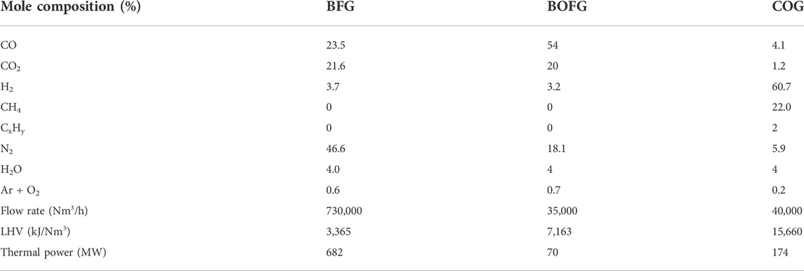
TABLE 1. The composition, amount, and heating value for each steel mill gas for a modern steel mill producing 6 Mt/yr of steel (Uribe-Soto et al., 2017).

Currently, these steel mill gases are either combusted to produce electricity or heat, or are flared, resulting in substantial GHG emissions and providing little economic value to the steel mill. It could be more cost-effective to obtain potentially valuable components such as CO and H₂ from steel mill gas than from conventional fossil-fuel-based or low-carbon sources, even after accounting for the value these gases provide to the steel mill in terms of heat and electricity (Collis et al., 2021). In most scenarios, it would also reduce the emissions of the steel mill, as the combustion of steel mill gas for electricity has a relatively high emissions intensity (0.64–0.82 tons-CO₂-eq./ton steel mill gas combusted) (Collis et al., 2021). CO and H₂ in particular can be mixed to create syngas, which can then be used as feedstock to produce fuels through a FT reaction.

2.2 Low-emissions solutions for aviation

The aviation sector is also under significant public and political pressure to cut emissions, as predictions state that emissions from the industry could double or triple from 2020 levels by 2050 (Gössling et al., 2021). There is a lack of promising technological options to reduce emissions from the industry in the short term. Three decarbonisation options are considered the most likely to become widely adopted; electric planes, hydrogen-powered planes, and the use of sustainable aviation fuel (SAF).

Electric planes require batteries with an energy density four to eight times higher than is currently possible and are only expected to see widespread use after 2040, firstly for smaller regional flights which make up less than 1% of global aviation emissions (Epstein and O’Flarity, 2019; Alexander et al., 2020; Krishnamurthy and Viswanathan, 2020). Take-off is also somewhat problematic for electric aeroplanes, as it requires significantly more thrust than coasting once in the air. With sufficient developments in battery technology, they could become the most efficient, quiet, and sustainable option for air travel in the long term future (Seeley et al., 2020). However, they will not make a significant impact in reducing GHG emissions from aviation in the next 2 decades.

Hydrogen-powered planes utilizing fuel cells are often mentioned as another possible low-emissions alternative. However, the energy density of H₂ (3.6 MJ/L) is significantly lower than that of aviation fuel (35.1 MJ/L). Gray et al. (2021) calculate that a fuel volume of 63,884 L of H₂ at 700 bar or 35,935 L of cryogenic H₂ would be required for short/medium-distance flights, compared with only 9,007 L of ordinary jet fuel. For long-distance flights, this translates to a required fuel mass of about 119% of the maximum take-off weight using compressed H₂ and 71.3% when using cryogenic H₂, while baseline jet fuel requires only 20.1% of the maximum take-off weight (Gray et al., 2021). Naturally, this excludes the possibility of H₂ for long-distance or even medium-distance flights with aeroplanes similar to those currently in use. Drastic design differences would be needed for hydrogen-powered planes to become viable.

SAFs are a promising option for short-to-mid-term emissions reduction. As they are designed to meet international jet fuel specifications, they can be used as a direct substitute for (or blended with) conventional fossil-fuel-based jet fuel. This avoids the need for changes to aircraft design and could potentially enable faster emissions reductions, as the currently operating aircraft fleet would not have to be phased out for new lower-emissions aircraft. Therefore, they are probably the most realistic option for short-term emissions reductions in the aviation industry.

Due to their low market share (0.01% in 2019) (IEA, 2019), there are several incentives by governments to increase the amount of SAFs used, which range from investment for production of SAFs to incentives for use in aircraft (Scheelhaase et al., 2019). Currently, Norway, Sweden, and France have a 1% SF blending requirement for aircraft in their territories, while the EU has announced targets of 2% by 2025, 5% by 2030, and 63% by 2050 (Malicier, 2022). The UK is even more ambitious, with targets of 10% by 2030 and 75% by 2050. California currently also incentivizes SAF blending (California Air Resources Board, 2020), and the US has introduced several policies such as a 1.5 USD/gallon credit for blenders supplying SAF, as well as a one billion USD grant to support SAF projects and producers (IATA, 2021).

SAFs can be produced through a variety of processes. Bio-based routes are some of the most technologically advanced routes, such as kerosene (jet fuel) produced from hydroprocessed esters and fatty acids (known as HEFA-SPK), which is commercially available with a technology readiness level (TRL) of 8 (Commercial Aviation Alternative Fuels Initiative, 2021). This process reacts renewable H₂ with alkenes and aromatics to form cycloalkanes and paraffins and currently makes up the largest fraction of SAFs used due to its technological readiness and low cost (1,100–1,350 €/tonne) (Bauen et al., 2020). Another bio-based process is the production of isoparaffins from hydroprocessed fermented sugars, also known as direct sugar to hydrocarbon routes (DSHC), which uses yeast or algae to convert sugar to hydrocarbons. This process has a TRL in the range of 7-8, indicating they are also close to industrial-scale production. However, this process is thus far comparatively expensive (4,000 €/tonne) (Bauen et al., 2020). Alcohol-to-jet (ATJ-SPK) is another promising process producing SAFs from biomass through fermentation of sugars to alcohols, with Yao et al. estimating relatively low costs of 1,080–1,550 €/tonne (Yao et al., 2017). Biomass pyrolysis to produce crude oil is also commercially available, but the process to refine pyrolysis oils to fuel is still in the demonstration phase (TRL 6). Additionally, biomass gasification followed by FT refining (FT-SPK) is nearing commercial readiness (TRL 7–8) (Im-orb et al., 2015), but faces difficulties with cost due to the small scale FT required for biomass process (IRENA, 2016). Currently, feedstock scarcity and land availability are major issues for scaling up bio-based SAF processes. To produce biomass at the scales required for aviation would require large quantities of land and water, which could heavily restrict its growth potential or have negative environmental impacts (Sheehan, 2009).

Other than bio-based SAF production, jet fuel produced from CO₂ and electrolytically produced H₂ (falling under the broad term of e-fuels) is another commonly assessed route (Ausfelder and Wagemann, 2020; Ramirez et al., 2020; Agarwal and Valera, 2022). This process uses water and electricity produced from renewable energy sources to produce H₂ in an electrolyser. Syngas (a CO and H₂ mixture usually made from coal or natural gas) is made from this H₂ and CO₂ (which could be captured from a point source or directly from the air) and is then reacted in a FT process and refined to produce aviation fuel (Hannula et al., 2020). The technology is not yet in industrial-scale commercial use (TRL 6–7), largely due to the currently high costs of electrolytic H₂ and the small scales of currently available electrolysers (Bauen et al., 2020). However, it is expected that costs for electrolytic H₂ will reduce in the future, which would make this process route more attractive, although it is yet unclear if it can be cost-competitive with conventional jet fuel (Glenk and Reichelstein, 2019). The high electricity and water demand are both an issue, as well as building the large electrolysers required to produce a substantial amount of jet fuel within the short time frames stated in the Paris agreement (Ueckerdt et al., 2021).

2.3 Fischer-Tropsch synthesis and refining

Fischer-Tropsch synthesis (FT) is a process that produces synthetic crude oil from syngas using metal catalysts. It is an established process and is mainly used in locations with extensive coal or gas reserves, but little oil, such as South Africa, which currently operates the largest FT plants. In the FT process, syngas enters a FT reactor where straight-chain alkanes are produced. Three main reactions occur in the FT reactor: the FT reaction, methanation, and water-gas shift (de Klerk, 2011a).

$CO+2H_2\to \left(-C{H}_2-\right)+H_{2}O$

$CO+3H_2\to C{H}_4+H_{2}O$

$CO+H_{2}O\to C{O}_2+H_2$

As well as alkanes, olefins, and oxygenates are formed in the FT reactor; however, these are usually disregarded in the reaction kinetics of most FT studies due to their low quality. The range of hydrocarbons produced in the FT reaction varies from chain lengths of one to over 100 carbon atoms and are usually modelled using the Anderson Schulz Flory (ASF) distribution, which uses a chain growth probability factor α (with 0 ≤ α ≤ 1) to determine the molecular distribution of hydrocarbon chain lengths (Albuquerque et al., 2019). The weight fractions of the molecular distribution are determined as follows (Hillestad, 2015):

$w_n=n{\alpha }^{n-1}{\left(1-\alpha \right)}^2$

where w_n is the weight fraction, n is the number of carbon atoms and α is the chain growth probability factor. The methanation reaction is shown separately from the FT reaction as short-chain hydrocarbons, and especially methane, are usually underrepresented in the ASF distribution. This can be rectified by either using two α values in the ASF distribution, one for C1-C10 hydrocarbons and one for C10+, or by including the methanation reaction as its own reaction, which then no longer depends on the ASF distribution to determine methane quantities.

FT processes can differ in several ways, with the main distinction being between low-temperature FT (LTFT) and high-temperature FT (HTFT). LTFT is operated between 220 and 250°C and produces alkanes with an α of approximately 0.94, which favours longer chain lengths, while HTFT is run between 320 and 350°C and has an α of around 0.7 ⁵². The ASF distribution by weight fraction for both HTFT and LTFT is shown in Figure 1. As well as the operating temperature, there are different catalyst possibilities for FT reactors, with cobalt and iron catalysts being commercially employed. Cobalt catalysts are effective at lower temperatures and pressures, but they cost up to 250 times more than iron catalysts (van de Loosdrecht et al., 2013), whereas iron catalysts are more tolerant to catalyst poisoning, but have a shorter lifetime than cobalt catalysts (Ma et al., 2020). The ratio of H₂ to CO in the feedstock syngas also impacts the reaction, with more short-chain hydrocarbons being produced as the relative amount of H₂ increases (Marchese et al., 2020). Lastly, three different reactor types can be used for the FT reaction; slurry-bed, fixed-bed, and fluidised-bed reactors. Fluidised-bed reactors can only be used for HTFT, in which the whole reaction phase is gaseous. Fixed-bed and slurry-bed reactors are used for LTFT, where liquid waxes are formed, which results in a three-phase system.

FIGURE 1

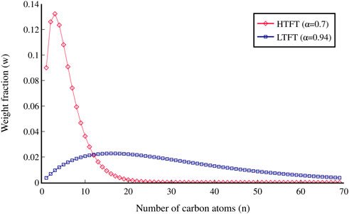
FIGURE 1. Anderson Schulz Flory distribution by weight fraction for alkanes of carbon numbers 1–70.

The synthetic crude oil from the FT reactor requires refining in order to produce valuable products such as jet fuel (de Klerk, 2008). Most jet fuel consumed is specified to the Jet A-1 standard, defined by the UK Ministry of Defence, which requires an aromatics content of 8%–25% and a minimum heat of combustion of 42.8 MJ/kg (Ministry Of Defence UK, 2011). Additionally, aviation fuel must have a sufficiently low freezing point to avoid freezing at the low temperatures reached at high altitudes (−47°C for Jet A-1). To achieve these characteristics, isomerisation of the paraffins produced by the FT reaction is required. To maximize yield from a jet fuel refinery, carbon numbers from C9–C16 are usually included, which have a boiling range from 149 to 288°C (De Klerk, 2010). The use of A-1 synthetic jet fuel has currently been approved for Sasol’s Secunda FT plant. LTFT is better suited for the production of jet fuel than HTFT, as it produces a greater fraction of alkanes in the longer chain length (kerosene) range, and the products have a higher level of hydrogenation and therefore require less hydrotreating (de Klerk, 2011b). The production of jet fuel compared to diesel from a FT process is advantageous from both a technical and economic perspective, due to the refinement complexities and low selling cost of producing diesel, as well as the growing demand for SAFs (de Klerk, 2009). It should also be noted, however, that FT syncrude requires more refining than mined crude oil due to the higher amounts of aromatic compounds in mined syncrude (de Klerk, 2008).

According to the process designed by de Klerk (De Klerk, 2010), refinement of LTFT syncrude to Jet A-1 requires three main conversion units; a hydrocracker, an aromatisation unit, and an alkylation/oligomerisation unit. The hydrocracker is used to break down longer hydrocarbon chains into molecules within the kerosene boiling range (C9–C16), and is responsible for 68% of total kerosene production within the refinery (de Klerk, 2011b). Additionally, isomerisation occurs, which helps lower the freezing point of the produced fuel. A platinum-loaded amorphous silica-alumina catalyst (Pt-Si-Al) is optimal for the hydrocracker due to its low methane selectivity in hydrogenolysis and the amorphous silica-alumina having high selectivity towards the formation of middle distillate (Calemma et al., 2001). The aromatisation unit uses a Zn or Ga-promoted H-ZSM-5 zeolite catalyst to convert paraffins and olefins from C5–C8 into aromatics (de Klerk, 2008). The addition of a metal species to form a bifunctional catalyst substantially increases the yield of aromatics in this unit (de Klerk et al., 2003). In the alkylation/oligomerisation unit, C9–C16 products are produced from light olefins (<C6) and aromatics (<C7) on a solid phosphoric acid (SPA) catalyst (Sakuneka et al., 2008). In this unit, two reactions occur: the alkylation reaction, which adds olefins to the aromatic compounds produced in the aromatisation unit to increase the fraction of compounds in the kerosene boiling range, and the oligomerisation reaction, in which olefins form a phosphoric acid intermediate that reacts with another olefin to form a longer olefin via the Langmuir–Hinshelwood mechanism (Mashapa and de Klerk, 2007). The complete FT refinement process for jet fuel production is shown in Figure 2.

FIGURE 2

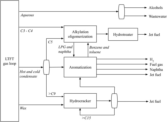
FIGURE 2. The refinement process for the production of jet fuel from a LTFT plant. Adapated from de Klerk (2011a).

3 Goal and scope

The goal of the study is to evaluate the economic and technical viability of producing jet fuel from steel mill gas in a FT process in southern France in 2022. Firstly, the entire process must be designed and simulated to ensure steel mill gas can be functionally used as a feedstock for a FT process. Secondly, a techno-economic assessment (TEA) will be conducted on the process to determine its economic viability. The minimum viable selling price (MVSP) of the fuel produced from the process described in this study will be compared to both fossil-fuel-based and renewable benchmarks (see section 3.1). Knowledge of the MVSP of the process is essential to both steel producers and aviation companies looking to reduce emissions. As the process aims to reduce the GHG emissions footprint of jet fuel, the process CO₂ emissions were also estimated so that they can be compared to the emissions footprint of conventional jet fuel and other SAF benchmarks.

In this study, steel mill gases COG and BFG from a French steel mill producing 8 Mt/y steel are mixed to create syngas, which is then fed into the FT process. COG has a high H₂ content, and BFG is a large stream with a moderate CO content, which are the primary components in syngas. These components are not captured from the steel mill gas, but rather BFG and COG are mixed directly and fed into the FT reactor. The type of FT is a LTFT process with an iron catalyst in a multi-tubular fixed-bed reactor. LTFT is optimal over HTFT for refinement of jet fuel (see section 2.3), and an iron catalyst was selected due to its low cost and immunity to NH₃ poisoning (de Klerk, 2011a). Fixed-beds offer high scalability and low complexity in comparison to slurry beds. The scope of the study is the entire FT process, from when steel mill gases are captured before they would otherwise have entered the combined heat and power plant (CHP) until the final product of jet fuel is produced, as highlighted by the dashed line boundary in Figure 3. BFG and COG require H₂S removal before being fed into the FT process, as N₂, CH₄ and CO₂ are effectively inert in the FT reaction (Jess et al., 1999). However, as steel mills are already required to remove H₂S and NH₃ before steel mill gases are combusted, these removal steps (the ‘steel mill gas treatment’ box in Figure 3) are considered to be out of the scope of this study. Additionally, further transport and storage of the jet fuel are not within the scope, as the associated costs would vary greatly depending on where the fuel would need to be transported. However, capture and storage (CCS) of the CO₂ emitted in the FT process is considered as an alternative scenario. The effects of a CO₂ tax on the process economics are also explored.

FIGURE 3

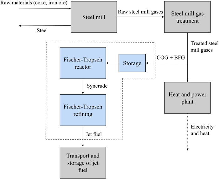
FIGURE 3. The scope of the study (the area in dashed lines) in the context of the larger supply chain. Essentially, the scope is from when steel mill gases are captured before combustion in the heat and power plant until when market-ready jet fuel is produced.

3.1 Benchmark definition

For jet fuel produced from steel mill gas (hereafter referred to as SMG-FT) to become adopted, it must be economically competitive with conventional and competing jet fuel production processes. The main benchmark for SMG-FT is conventional fossil-fuel-based jet fuel. Conventional jet fuel fluctuates in price significantly with the crude oil price, particularly since 2020 due to the COVID-19 and Ukraine war crises (IATA, 2022). For example, the average jet fuel price in 2020 was around 325 €/tonne (Jet-A1-Fuel, 2020) due to an extremely low crude oil price, whereas in 2021 the average jet fuel price rose to 551 €/tonne (Jet-A1-Fuel, 2021) and is currently averaging 955 €/tonne through the first 5 months of 2022 (IATA, 2022). For this study, the average price from January 2018 to January 2022 (598 €/tonne) will be taken as the main benchmark for comparison. It is also overall more in line with pre-2020 jet fuel costs, which were more stable than prices from 2020 to 2022 (558 €/tonne in 2019 ⁶⁸, 601 €/tonne in 2018 ⁶⁹).

Although fossil-fuel-based jet fuel may have the lowest MVSP well into the future, government incentives and CO₂ taxes could make SAFs cost-competitive within a much shorter time frame. Mandates on low-emissions fuel blending could also enforce the uptake of SAFs even before they are cost-competitive. Therefore, the SMG-FT process must also be benchmarked against other SAFs.

There is an abundance of TEAs on SAF production, most of them focusing on bio-based routes (Wang, 2016; Yao et al., 2017; Baral et al., 2019; Martinez-Hernandez et al., 2019; Tongpun et al., 2019; Eswaran et al., 2021; Mousavi-Avval and Shah, 2021; Peters et al., 2022). Several SAF benchmarks are chosen for this study, as it is unclear which technology will become the most dominant and it is likely that multiple process routes will be used to produce SAFs for some time. Dahal et al. (2021) reviewed 26 economic assessments on SAF production and summarised the results; the MVSP ranges they found are used as a basis for the SAF benchmarks selected in this study, with more recent additional studies added to their dataset. The range of MVSPs found in the literature for the SAF benchmarks is shown in Table 2, along with the range of conventional jet fuel prices recorded from 2018 to 2021. The different processes themselves are discussed in more detail in section 2.2.

TABLE 2

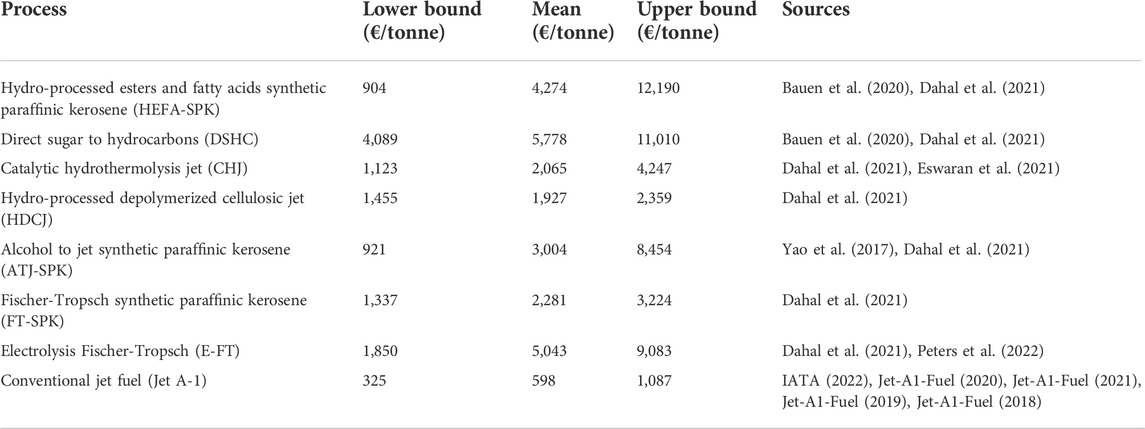
TABLE 2. MVSP ranges for the SAF benchmarks selected for the study.

As well as economic benchmarks, GHG emissions benchmarks are also necessary, as stakeholders are likely to purchase and produce SAFs primarily because of the lower GHG emissions when compared to conventional jet fuel. Conventional, fossil-fuel-based jet fuel has life-cycle emissions of around 88 gCO_2eq/MJ (De Jong et al., 2017). Several SAFs are also selected as GHG emissions benchmarks and are shown in Table 3.

TABLE 3

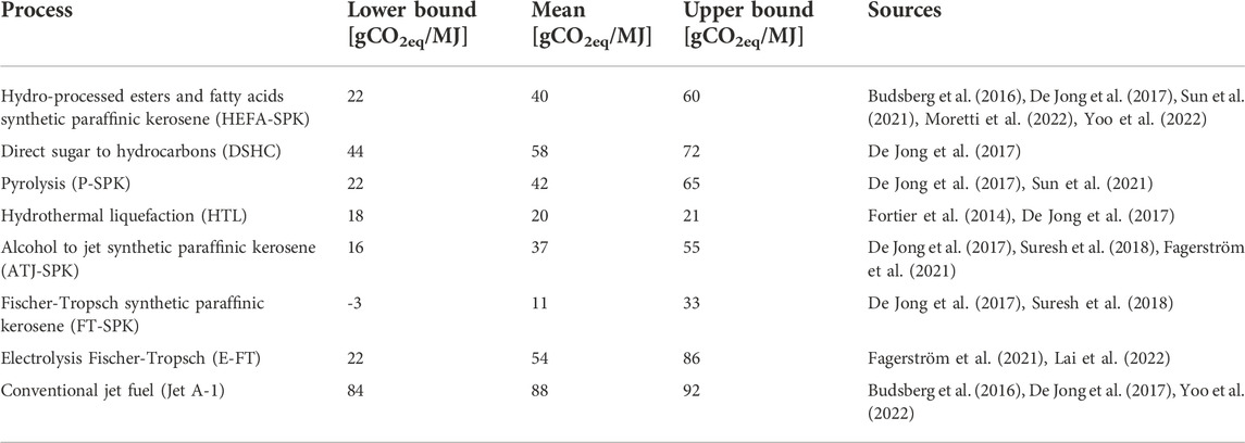
TABLE 3. GHG emissions for the SAF benchmarks selected for the study showing cradle-to-gate emissions.

4 Process modelling

4.1 Fischer-Tropsch synthesis

4.1.1 Reaction conditions and feedstock properties

The complete FT process outlined in three was modeled as a stationary continuous process in Aspen Plus V10, with additional calculations done in Berkeley Madonna (Marcoline et al., 2022). Firstly, the amount of feedstock gas to the FT process was determined. A BFG stream of 1,000,000 Nm³/h and a COG stream of 70,000 Nm³/h were assumed from a steel mill producing 8 Mt/y steel. As the BFG stream is much larger, the size of the COG stream is the limiting factor for the amount of jet fuel that can be produced from a steel mill. A syngas H₂/CO ratio of 1.75 is optimal to produce the chain lengths best suited for jet fuel production (de Klerk, 2011a). The amount of the BFG stream to be captured was then calculated according to this optimal ratio:

$V_{BFG}=V_{COG}\frac{x_{H_2,COG}-1.75x_{CO,COG}}{{{1.75x}_{CO,COG}-x}_{H_2,BFG}}$

where V is the volume flow and x is the mole fraction. The amount of BFG required and the composition of the mixed gas are shown in the Supplementary Table S1.

The BFG and COG streams are cooled before compression to the reaction pressure, through which the H₂O condenses and is removed. The methanation reaction is not reversible under standard FT reaction conditions and thus additional CH₄ in the feed stream is effectively inert in the reaction. It is therefore not necessary to remove the CH₄ from the COG before it enters the reactor. CO₂ and N₂ can also be regarded as inert for LTFT (Jess et al., 1999).

The reaction simulation was based on the experimentally verified model derived by Jess et al. (1999); Jess and Kern (2009), with the same inlet temperature of 240°C (513.15 K) being selected. A plug flow tube reactor (PFTR) model was chosen to model the behaviour of the FT tubular fixed-bed reactor. Two reactors in series were chosen to ensure sufficient conversion to the desired products. Next, the pressure in the first reactor was calculated based on the partial pressure of CO in the reactor modelled by Jess and Kern (2009) (overall reactor pressure 24 bar):

$p=\frac{{RTc}_{CO,\mathit{mix}}}{x_{CO,\mathit{mix}}}$

where R is the ideal gas constant (8.314 J/mol K), T is the inlet temperature (513.15 K), c_CO,mix is the CO concentration at 24 bar (187.52 mol/m³), and x_CO,mix is the mole fraction of CO in the mixture (0.16), resulting in a reactor pressure of 49.5 bar. The reactor dimensions must also be specified. Tubes with a length (z) of 8 m and diameter (d_int) of 7 cm were selected and the residence time (τ) of the first reactor was chosen to be 25 s (Jess et al., 1999). The inlet surface velocity (u_s,0 = z/τ) and reactor volume (V = V̇τ) can then be calculated.

The distribution of the product exiting the FT reactor is calculated using the ASF distribution (see Fischer-Tropsch synthesis and refining), for which an α value of 0.934 was selected, resulting in 52 wt% of C22 + straight chain alkanes (de Klerk, 2011a). Each produced alkane chain is further divided into olefins, isomers, and oxygenates according to ratios defined in literature (Hoogendoorn, 1975; Dry, 1981).

4.1.2 Kinetic modelling

LTFT-specific rate equations with CO as the key component have been derived from experimental work (Kuntze et al., 1995; Raak and Hedden, 1998). The effective rate constants (k_0,CO,eff) include pore diffusion mass transfer limitations under reaction conditions and are valid for a temperature range of 170–400°C for catalyst particles of 2.5 mm diameter (Jess et al., 1999). They are shown below for each of the three reactions occurring in the FT reactor (FT reaction, methanation, and water-gas shift reaction):

$r_{FT}=\frac{{d\dot{n}}_{CO}}{d{m}_{\mathit{c}\mathit{a}\mathit{t}}}=\frac{k_{0,CO,eff,FT}{e}^{-\left(\frac{E_{A,FT}}{RT}\right)}{c}_{H_2}}{1+1.6c_{H_{2}O}/c_{CO}}$

$r_M=\frac{{d\dot{n}}_{CO}}{d{m}_{\mathrm{c}\mathit{a}\mathit{t}}}=k_{0,CO,eff,M}{e}^{-\left(\frac{E_{A,M}}{RT}\right)}{c}_{H_2}$

$r_{Sh}=\frac{{d\dot{n}}_{CO}}{d{m}_{\mathit{c}\mathit{a}\mathrm{t}}}=k_{0,CO,eff,Sh}{e}^{-\left(\frac{E_{A,Sh}}{RT}\right)}{c}_{H_{2}O}$

where r is the rate of reaction (mol/kg s), ṅ is the molar flow (mol/s), m_cat is the catalyst mass (kg), k_0,CO,eff is the effective rate constant (m³/kg s), c is the concentration (mol/m³), E_A is the activation energy (J/mol), R is the ideal gas constant (8.314 J/mol K), and T is the temperature (K). The reaction constants for the above rate equations are specified in the Supplementary Table S2.

Next, the mass balances were established. To calculate the change in concentration along the reactor (dc/dz), the rate of reaction (r) was multiplied by the catalyst bulk density (ρ_b) and divided by the surface velocity (u_s) to convert time dependency to location dependency, as shown below for each component.

$\frac{{dc}_{CO}}{dz}=\frac{{\rho }_b}{u_s}\left(-r_{FT}-r_M-r_{Sh}\right)$

$\frac{{dc}_{H_2}}{dz}=\frac{{\rho }_b}{u_s}\left(-\left(3-\alpha \right)r_{FT}-3r_M+r_{Sh}\right)$

$\frac{{dc}_{H_{2}O}}{dz}=\frac{{\rho }_b}{u_s}\left(r_{FT}+r_M+r_{Sh}\right)$

The change in molar flow (dṅ/dt) as the reactions consume more of the reactants was then determined:

$\frac{dṅ}{dt}={S\rho }_b\left(-2r_{eff,FT}-2r_{eff,M}\right)$

where S is the surface area of the reactor (m³), ρ_b is the catalyst bulk density (kg/m³), and r_eff is the rate of reaction for each of the reactions (mol/kg s). The change in surface velocity (u_s) and molar density (ρ_mol) can then also be calculated:

$u_s=\frac{\dot{n}RT}{pS}$

${\rho }_{\mathit{mol}}=\frac{p}{RT}$

4.1.3 Heat transfer in the reactor

Heat transfer in the reactor is important to understand as it affects the reaction rate. Heat transfer along the reactor was modelled using the one-dimensional axial model by Jess and Kern (2009):

$\frac{dT}{dz}=\frac{{4U}_0\left(T_C-T\right)}{d_i{\rho }_{\mathit{mol}}{c}_p{u}_s}-\frac{{\rho }_B\sum \left({∆}_R{H}_i{r}_{eff,i}\right)}{{\rho }_{\mathit{mol}}{c}_p{u}_s}$

where U₀ is the overall heat transfer coefficient (W/m² K), T_C is the temperature of the cooling liquid (K), c_p is the heat capacity of the gas mixture (J/mol K), ρ_mol is the molar gas density (mol/m³), Δ_RH is the enthalpy of reaction (J/mol), and r_eff is the effective rate of reaction (mol/kg s). The overall heat transfer coefficient (U₀) was determined by summing the heat transfer through the bed, wall, and the cooling medium:

$U_0={\left(\frac{d_{\mathit{int}}}{8{\lambda }_{rad}}+\frac{1}{{\alpha }_{w,\mathit{int}}}+\frac{d_{wall}}{{\lambda }_{wall}}+\frac{1}{{\alpha }_{w,ext}}\right)}^{-1}$

where d_int is the internal diameter of the tubes (m), λ_rad is the radial heat conductivity (W/m K), α_w is the heat transfer coefficient of the wall (W/m² K), d_wall is the wall thickness of the tubes (m), and λ_wall is the heat conductivity of the wall (W/m K). The internal wall heat transfer coefficient (α_w,int) and radial heat conductivity (λ_rad) are dependent on the catalyst particle size and geometry, as well as fluid stream parameters, and were calculated using the following empirical equation (Jess and Wasserscheid, 2013):

${\alpha }_{w,\mathit{int}}=\frac{{\lambda }_{fluid}}{d_p}\left[4\left(1.3+\frac{5d_p}{d_R}\right)+0.9{Re}_p^{0.75}{\mathit{Pr}}^{\frac{1}{3}}\right]$

${\lambda }_{rad}={\lambda }_{fluid}\left(4+\frac{{Re}_p\mathit{Pr}}{4.6\left[2-{\left(1-\frac{2d_p}{d_r}\right)}^2\right]}\right)$

where λ_fluid is the heat conductivity of the fluid (W/m K), d_p is the catalyst particle diameter (m), d_R is the cross-sectional diameter (m), Re is the Reynolds number (dimensionless) and Pr is the Prandtl number (dimensionless). The cross-sectional diameter used in the above formulas (d_R) is effectively the diameter of a single tube with the equivalent cross-sectional area of all tubes:

$d_R=\sqrt{n{d}_{\mathit{int}}^2}$

where n is the number of tubes (dimensionless). The complete set of parameters used in the above formulas are shown in the Supplementary Table S5.

4.1.4 Implementation of reactor simulation

An Rplug model with Langmuir–Hinshelwood Hougen-Watson (LHHW) type reactions was used in Aspen Plus to represent the FT reactors. The rate parameters shown in Supplementary Table S5 were entered for each reaction, and the products were set according to the ASF distribution defined in Reaction conditions and feedstock properties. To simplify the model for Aspen Plus, C22 + components were lumped together into one component by taking the average fraction and molecular weight of all alkanes from C22 to C200 (Hillestad, 2015). Stoichiometric coefficients (υ) for each alkane were used to specify the reaction and were calculated as follows:

${\upsilon }_n={\alpha }^{n-1}{\left(1-\alpha \right)}^2$

where n is the number of carbon atoms. The catalyst mass and the number of tubes for both reactors (Supplementary Table S5) were also parameters for the Rplug model in Aspen. The heat transfer calculations were carried out externally in Madonna and the determined temperature profile was entered into Aspen. A pressure drop of 2 bar in each reactor was assumed and was introduced at the reactor outlet in Aspen (de Klerk, 2011a). The redistribution of alkanes was done in a subsequent Ryield reactor model to include other hydrocarbon species.

4.2 Fischer-Tropsch jet fuel refining

After the second FT reactor, the gas is cooled to 30°C and flashed at 45.5 bar to separate the water, the middle-distillate syncrude fraction, and the gas into different streams. The gas stream then enters a membrane separation unit to recover propene and butene, which are sent to the alkylation unit (de Klerk, 2011a). The main inlet streams for the jet fuel refinery section are the middle distillate and the wax stream. In a distillation column, the middle distillate stream is split up into > C9 and <C9 hydrocarbon fractions, which are sent to the hydrocracker and aromatisaion unit respectively, as shown in Figure 2.

4.2.1 Hydrocracker

The complete refinery was modelled in Aspen Plus in the same simulation as the FT reactor highlighted in Fischer-Tropsch synthesis. As mentioned in section 2.3, the hydrocracker is employed to split longer (C22+) chain lengths into shorter ones (C3-C19) and is responsible for 68% of the output of a FT jet fuel refinery (de Klerk, 2011b). Operating conditions of 260°C and 30 bar were selected (Sun et al., 2017). An ideal hydrocracker model, as described by Bouchy et al. (2009), was used to calculate the reactor stoichiometry. This model assumes no C1-2 components are produced (and hence also no Cn-1 and Cn-2 components, where n is the number of carbon atoms of the cracked component). Molar amounts of C3 and Cn-3 are assumed to be half the amount of the rest of the components in the C4 to Cn-4 range, as per the example shown in Figure 4 for 1 mol of cracked C22.

FIGURE 4

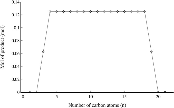
FIGURE 4. Product distribution resulting from 1 mol of cracked C22 using the ideal hydrocracking model (Bouchy et al., 2009).

An atomic balance was then used to calculate the products for each chain length that is cracked from C22-C200:

$n_{4,N_{crack}}=\frac{n_{in}{N}_{crack}}{\frac{N_{c,3}+N_{c{,N}_{crack}-3}}{2}+{\displaystyle \sum }_{i=4}^{N_{crack}}{N}_{c,i}}$

where n_i is the amount of cracking product (mol), N_c,i is the carbon number of cracking product (unitless), N_crack is the carbon number of the component being cracked (unitless), and n_in is the feed amount of component being cracked (mol). Each N_crack carbon number in the C22 + lump results in a n_4,Ncrack value, which in turn is used to calculate the molar product distribution between C3 and CN_crack-3. The molar amounts of the cracked products are calculated by summing up the n_4,Ncrack values from C3 to C198, as shown in the following three equations:

$n_{C3}={\displaystyle \sum }_{i=22}^{200}{\frac{1}{2}n}_{4,i}$

$n_{C4-C18}={\displaystyle \sum }_{i=22}^{200}{n}_{4,i}$

$n_{19+}=\frac{n_{4,N_{crack}}}{2}+{\displaystyle \sum }_{i=N_{crack}+1}^{200}{n}_{4,i}$

After the hydrocracker, a distillation column is used to separate C17 + components from those in the jet fuel boiling range. The C17 + components are then recycled through the hydrocracker to increase conversion.

4.2.2 Aromatisation unit

Chain lengths C1-C8 are fed into the aromatisation unit, where C5-C8 paraffins and olefins are converted to aromatics. The product distribution is determined separately for each chain length based on experimental studies (Viswanadham et al., 2004; Song et al., 2014; Liu et al., 2015), and is shown in the Supplementary Table S3. Reaction conditions of 500°C and 5 bar were selected as mid-points from the experimental studies. H₂ is also formed in the aromatization unit but is not included in the results of the experimental studies; the amount of H₂ produced was determined using a molecular balance. While the experiments used different catalysts, the product distributions resulting from both Ga and Zn loaded ZMS-5 catalysts are similar and the results from these experiments can therefore both be used.

4.2.3 Alkylation unit

In the alkylation unit, C3-C5 aliphatic olefins, benzene, and toluene are reacted to form n-propylbenzene and n-pentylbenzene. An operating pressure of 38 bar and temperature of 200°C were chosen based on commercial FT plants (Mashapa and de Klerk, 2007; de Klerk, 2011a). Similarly to the aromatization unit, the reaction products are determined from literature values (de Klerk, 2011a) based on the ratio of toluene and benzene in the feedstock and are shown in the Supplementary Table S4.

4.3 Techno-economic assessment

The techno-economic assessment (TEA) was performed according to established guidelines (Buchner et al., 2018; Zimmermann et al., 2020). Capital expenditure (CapEx) was determined on an individual equipment cost basis using the method outlined by Towler and Sinnott (2017):

$C_e=a+b{S}^n$

where C_e is the purchased equipment cost (2007 USD at the Gulf Coast), S is a unit-operation-specific size dimension, and a, b, and n are unit-operation-specific constants. The dimensions of the major equipment and purchased equipment cost for each unit operation are shown in the Supplementary Tables S6, S7. The costs for the two FT reactors were determined separately using a cost diagram by Garrett (2012); they were assumed to be multitubular heat exchangers. Location, currency conversion, and chemical engineering plant cost index (CEPCI) factors were applied to convert the equipment costs from 2007 USD at the Gulf Coast to 2022 Euros in Western Europe (Towler and Sinnott, 2017). Once the purchased equipment costs in 2022 Euros were determined, they were multiplied by installation factors and summed together to calculate the total inside battery limits (ISBL) cost (Towler and Sinnott, 2017):

$C={\displaystyle \sum }_{i=1}^M{C}_{e,i}\left[\left(1+f_p\right)f_m+f_{er}+f_{el}+f_i+f_c+f_s+f_l\right]$

where M is the number of unit operations, f_m is the materials factor for carbon steel (1), f_p is the piping installation factor (0.8), f_er is the equipment erection installation factor (0.3), f_el is the electrical installation factor (0.2), f_i is the instrumentation installation factor (0.3), f_c is the civil engineering factor (0.3), f_s is the installation factor for structures and buildings (0.2), and f_l is the lagging, insulation or paint installation factor (0.1). Next, the total invested capital (C_FC) was determined by applying further factors for contingency (X = 0.1), off-sites (OS = 0.3) and design and engineering (D&E = 0.3) to the ISBL cost C (Towler and Sinnott, 2017):

$C_{FC}=C\left(1+OS\right)\left(1+D\&E+X\right)$

Operational expenditure (OpEx) consists of three main cost areas; material costs, utility costs, and labour/maintenance costs. Labour costs were calculated using the method outlined by Turton et al. (2008):

$N_{Op}=\sqrt{6.29+0.23\sum N_e}$

where N_Op is the number of operators required to run the plant at any given time, and N_e is the number of unit operations (37 for the studied FT process). The number of operators is multiplied by 4.5 to cover constant plant operation over a year (Turton et al., 2008); operators are assumed to work 2,000 h a year at a cost of 38.6 €/h (Ministere de l’Économie et des Finances, 2017). Further supervision and maintenance costs are applied as factors of the labour cost and ISBL and are shown in Table 4.

TABLE 4

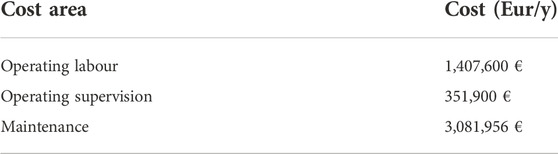
TABLE 4. Maintenance and labour costs for the process in 2021 Euros (Towler and Sinnott, 2017; Turton and Shaeiwitz, 2017).

Material costs were determined from current market prices; all chemicals required except the steel mill gas are traded in reasonable large volumes. The purchase cost of BFG and COG was determined from the value they provide to the steel mill in heat and power generation, which is based on their calorific values (Collis et al., 2021). The cost of the hydrocracker catalyst was determined by the price of the catalyst support and the market price for platinum. The assumed utility and material costs are shown in Tables 5, 6 respectively.

TABLE 5

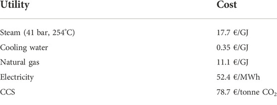
TABLE 5. Assumed utility costs for the process in 2021 Euros (Naims, 2016; PWC, 2016; Turton and Shaeiwitz, 2017).

TABLE 6

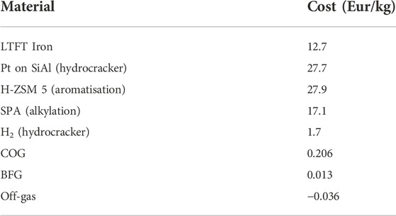
TABLE 6. Material costs for the process in 2021 Euros (Hanaoka et al., 2015; Collis et al., 2021; Zauba; Broker, 2022). Off-gases from the process are re-sold to the steel mill for heat and electricity generation.

The net present value (NPV) was used as a second profitability indicator; it represents the value of all future cash flows in the current time period. The discounted cash flow (DCF) for a certain time period is calculated as follows:

$DCF=\frac{CF}{{\left(1+i\right)}^t}$

where i is the discount rate and t a given time period. The NPV was then calculated in a cash flow table, where discounted cash flows are summed every year over the number of years assumed as the time period. The baseline sales price chosen was the median benchmark for conventional fossil-fuel-based jet fuel (2021 average). The list of assumptions used for the NPV calculations is shown in Table 7.

TABLE 7

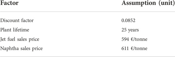
TABLE 7. List of assumptions for the NPV calculation (Jet-A1-Fuel, 2021; Damodaran, 2019; Börse, 2022).

4.4 GHG emissions assessment

A full life-cycle assessment (LCA) is outside the scope of the study; however, a simple cradle-to-gate CO₂ emissions balance was performed. As the steel mill is producing steel in any case, the life-cycle emissions of the steel mill are allocated to the steel product and not to the SAF produced. The only emissions from the steel mill that must be factored in are electricity grid emissions required to replace the electricity that would have otherwise been produced by the steel mill gas (Collis et al., 2021). The amount of CO₂ emissions produced through FT synthesis were determined from the Aspen Plus simulation. The CO₂ emissions produced by the combustion of natural gas are:

${\dot{m}}_{{CO}_2}={\dot{n}}_{{CH}_4}\left(1+\frac{2M_{O_2}-2M_{H_{2}O}}{M_{{CH}_4}}\right)$

Full oxidation of hydrocarbons in the FT off-gas stream is assumed. A CCS cost of 79 €/tonne is assumed, along with a capture rate of 90% (Kheshgi et al., 2012; Panja et al., 2022). Additional CO₂ is produced from the consumption of CH₄ and the production of H₂ needed in the process, as well as the electricity uses of the process.

As well as determining the emissions intensity of the produced fuel, an emissions assessment was carried out from the perspective of the steel mill, to determine if the overall emissions of the steel mill could be decreased using the SMG-FT process compared to conventional steel mill gas usage. This assessment compared the yearly emissions of the total SMG-FT process to the yearly emissions of the benchmark steel mill, if the steel mill gas that would be used for the SMG-FT process is instead combusted as normal in a heat and power plant.

5 Results

5.1 Simulation results

A total of 51.2 kt/y of jet fuel and 2.5 kt/y of naphtha are produced from the modelled process. The jet fuel has an aromatics content of 11% and an energy content of 43.7 MJ/kg, which fulfils the minimum requirements of the jet fuel A1 standard (see section 2.3). Of the total amount, 88% is produced in the hydrocracker, 8% from the aromatisation unit, and 4% from the alkylation unit. The combined conversion of the two FT reactors is 44%, with a 24% hydrocarbon yield, and the yield of the refinery is 82%. Using the heat transfer modelling presented in section 4.1.3, the temperature changes along both FT reactors were derived (Figure 5). The temperatures are set to stay below 250°C to allow a slight buffer, as the iron catalyst begins to deactivate at 260°C (Jess et al., 1999). The temperature of the inlet feed in reactor 2 is 10°C lower than the inlet to reactor 1 to account for the increased residence time (from 25 s in reactor 1 to 37 s in reactor 2, to ensure conversion remains as high as possible).

FIGURE 5

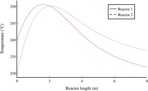
FIGURE 5. Temperature changes along both FT reactors.

Similarly, the conversion of each modelled reaction was determined using the reaction kinetics outlined in section 4.1.2 (Figure 6). The overall conversion of CO in the second reactor is 48% compared to 36% in reactor 1. This increase is mainly a result of the WGS reaction, which accounts for 18% of the conversion in the second reactor and is caused by the increased water concentration at the inlet. The FT reactor setup presented in literature (Jess et al., 1999) proposes the separation of water after the first reactor. This solution was dismissed for this study due to the extensive energy requirement for condensation and reheating of the large gaseous feed stream to reactor 2.

FIGURE 6

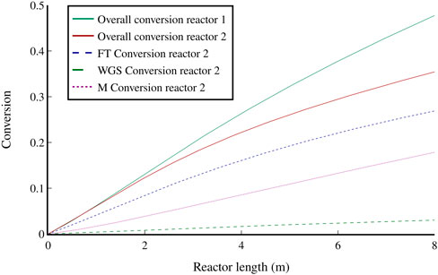
FIGURE 6. The overall conversion of CO in both FT reactors and conversion of each modelled reaction in the second FT reactor: Fischer-Tropsch (FT), Water-gas shift (WGS), and methanation (M).

5.2 Techno-economic assessment

Both static (MVSP) and dynamic (net present value) profitability indicators are used to assess the economic viability of the process. The MVSP (production cost) of the process was found to be 1,046 €/tonne, which is comparable to the lowest costs found for other SAF routes, although higher than that of conventional jet fuel, as shown in Figure 7. It is similar in cost to fuels produced from other FT processes; for example, fuel from coal gasification has a production cost of 981 €/tonne (Trippe et al., 2013). For the scenario with CCS, the cost was found to be 1,150 €/tonne. Among other SAF process routes, only the lowest costs found for the HEFA-SPK (904 €/tonne) and ATJ-SPK (921 €/tonne) routes were lower than the calculated cost for the SMG-FT route, and the average costs found for those routes (4,274 €/tonne and 3,004 €/tonne respectively) are well above the calculated cost for the SMG-FT route (Yao et al., 2017; Bauen et al., 2020; Dahal et al., 2021). The high MVSP volatility of these bio-based process routes is likely due to the different feedstock costs and other assumptions made by the various studies. The SMG-FT route also offers a lower jet fuel MVSP than the lowest bio-based FT process found [1,337 €/tonne (Dahal et al., 2021)]. The most heavily-investigated non-bio route, E-FT, has a minimum found MVSP of 1,850 €/tonne (Peters et al., 2022), which is 57% higher than the calculated cost of the SMG-FT route. As well, the E-FT route has a large range of reported prices, with the median found MVSP being 5,043 €/tonne (Dahal et al., 2021), likely due to the high uncertainty of economic assessments on H₂ electrolysis and CO₂ capture technologies (Collis and Schomäcker, 2022).

FIGURE 7

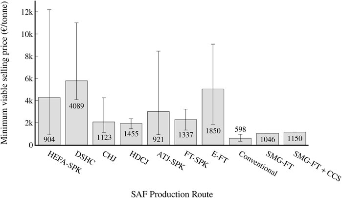
FIGURE 7. MVSP (production cost) of the various SAF benchmarks (see Benchmark definition) and conventional aviation fuel. The grey bar represents the median cost found for each process route among studies, while the error bars correspond to the lowest and highest cost found for each process route. The text states the lowest found cost for each production route.

The net present value (NPV) of the plant assuming no CO₂ tax if the product was to be sold at the benchmark (2021) price of conventional jet fuel is -173 M€ for the standard scenario and −209 M€ with CCS, and both scenarios record a loss in yearly expenses. These figures increase to −3.03 M€ and −39.3 M€ respectively when using current (2022) jet fuel prices, and a yearly profit is recorded with a payback time of 7.9 years for the standard scenario and 11.5 years for the CCS scenario. However, there have been no SAF processes found that have a lower MVSP than conventional jet fuel, and most SAF techno-economic assessments assume that some form of subsidy or CO₂ tax will be applied to make SAFs more competitive with conventional jet fuel. Both the NPV and MVSP of the SMG-FT process are analysed with various assumed CO₂ taxes in section 5.4.

Figure 8 highlights the contribution from various cost sources to the overall MVSP for the CCS scenario. The largest cost contributors are the electricity usage (174 €/tonne), the purchase of steel mill gas from the steel mill (423 €/tonne), and the annualised capital cost investment (281 €/tonne). Compressors comprise the biggest portion of electricity usage in the plant, particularly the two largest compressors before the FT reactor. COG is the most costly steel mill gas to purchase from the steel mill, as it has the highest energy content and is therefore the most useful for the production of heat and electricity (Collis et al., 2021). Meanwhile, the two first compressors, the FT reactors, and the membrane module require the largest capital investment.

FIGURE 8

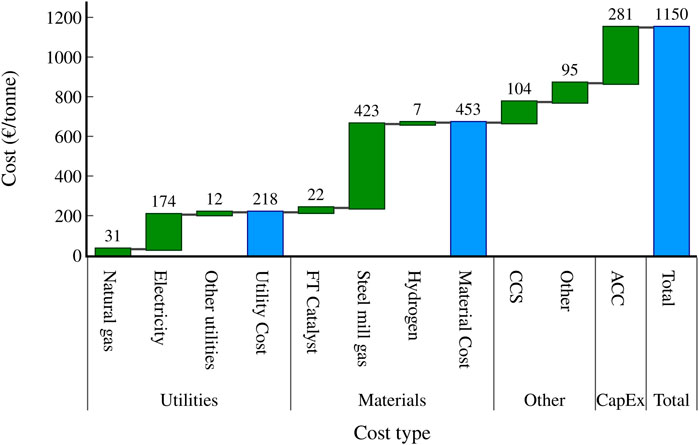
FIGURE 8. Waterfall graph highlighting the biggest contributors to the MVSP for the scenario with CCS.

5.3 GHG emissions assessment

A total of 107.6 kt CO₂-eq./y (49.7 gCO₂-eq./MJ) is produced by the studied process, and when CCS is considered, the process produces 46.7 kt CO₂-eq./y (21.1 gCO₂-eq./MJ). Both scenarios have significantly lower emissions intensity than conventional jet fuel (84–92 gCO₂-eq./MJ (Budsberg et al., 2016; De Jong et al., 2017; Yoo et al., 2022). The normal scenario has similar emissions intensity to DSHC and E-FT processes, which have a reported average of 42 gCO₂-eq./MJ and 54 gCO₂-eq./MJ respectively, but range from 22–86 gCO₂-eq./MJ (De Jong et al., 2017; Suresh et al., 2018). It has an emissions intensity within the found bounds of the other studied SAF production routes, except for FT-SPK and HTL, as shown in Figure 9. The CCS scenario has a much lower emissions intensity and is comparable to or lower than the lowest found emissions from all process routes except FT-SPK. The FT-SPK route has a lower bound of -3 gCO₂-eq./MJ, but upper bound of 33 gCO₂-eq./MJ, meaning that the studied SMG-FT process route could indeed still be competitive with the FT-SPK route in terms of GHG emissions. The process routes with the next lowest found emissions intensities are ATJ-SPK (16 gCO₂-eq./MJ), HEFA-SPK and E-FT (22 gCO₂-eq./MJ), and HTL (18 gCO₂-eq./MJ). However, each of these routes other than HTL has a large range of reported emissions intensities. Therefore, the lowest reported emissions intensities may be more uncertain or only for specific case studies or scenarios. On the other hand, HTL has a low reported range of only 18–21 gCO₂-eq./MJ, and is the only process route found where the maximum reported emissions intensity is lower than the emissions intensity of the CCS SMG-FT scenario.

FIGURE 9

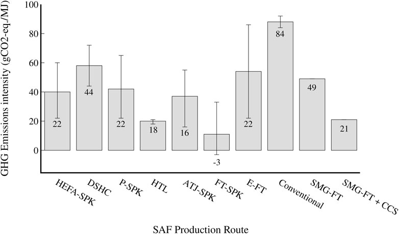
FIGURE 9. GHG emissions intensity (gCO₂-eq./MJ jet fuel) of the various SAF benchmarks (see section 3.1) and conventional aviation fuel. The grey bar represents the median GHG emissions found for each process route among studies, while the error bars correspond to the lowest and highest GHG emissions found for each process route. The text states the lowest found GHG emissions for each SAF production route. A capture rate of 90% is assumed for the CCS scenario.

Figure 10 shows the contributions of different feeds and process sections to the overall emissions intensity for the CCS scenario. The biggest emissions contribution is the FT synthesis itself (30.5 gCO₂-eq/MJ), which is similar to other FT-based SAF routes (De Jong et al., 2017). The H₂, CH₄, and electricity required as well as the emissions required to replace the usages of steel mill gas in the steel mill together contribute 18.2 gCO₂-eq/MJ, with the steel mill gas itself making up the largest portion of that at 10.4 gCO₂-eq/MJ. With CCS used to capture the emissions from the FT reactors, the total process emissions can be reduced by 27.6 gCO₂-eq/MJ, assuming a capture rate of 90%.

FIGURE 10

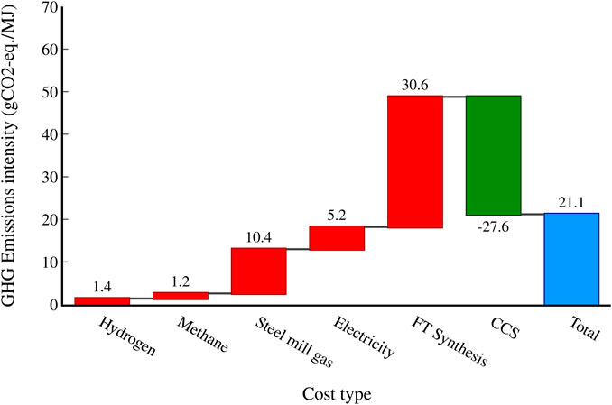
FIGURE 10. Waterfall graph highlighting the contributions of different process segments to the overall process emissions intensity for the scenario with CCS. A capture rate of 90% is assumed.

The yearly emissions of different process elements to the overall emissions for the CCS process are shown in Figure 11, along with the emissions of the benchmark steel mill, assuming the steel mill gases that would have been used for the SMG-FT process were combusted as normal in a heat and power plant. The CCS process reduces the total yearly emissions from the steel mill by 191 ktCO₂-eq./y if a capture rate of 90% is achieved, while the standard process would reduce the emissions by 130 ktCO₂-eq./y. It should be noted that the benchmark emissions of 1,030 ktCO₂-eq./y are only the emissions of the amount of steel mill gas that would be sent to the SMG-FT process, not the total emissions of the steel mill.

FIGURE 11

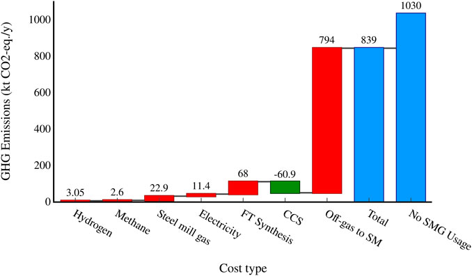
FIGURE 11. Waterfall graph showing the yearly emissions from different process segments and the total yearly process emissions compared to the yearly emissions if the steel mill ran as normal. A capture rate of 90% is assumed.

5.4 CO₂ tax assessment

Many SAF TEA and LCA studies account for a CO₂ or GHG emissions tax, as without either economic incentives or government mandates it is currently unfeasible for SAFs to economically compete. For this study, a CO₂ tax of 130 €/tonne was implemented, which is roughly in line with projections for the EU emissions trading scheme (ETS) in 2030 (Pietzcker et al., 2021). Figure 12 shows the MVSP of those SAF benchmarks for which both an economic and environmental benchmark were found, as well as conventional jet fuel, account for a CO₂ emissions tax of 130 €/tonne CO₂-eq. emitted. The CO₂ tax increases the MVSP of both the standard SMG-FT process (1,320 €/tonne) and the SMG-FT process with CCS (1,269 €/tonne), although the increase for the CCS process is substantially less as it has significantly lower process emissions. The addition of the CO₂ tax brings the MVSP for conventional fossil fuels (797–1,604 €/tonne with the average being 1,092 €/tonne) into the same cost range as the SMG-FT process. With such a tax, the CCS scenario could potentially be economically competitive with conventional jet fuel, and would be significantly lower than the current jet fuel price. Other SAFs also remain competitive, with HEFA-SPK (1,028 €/tonne), ATJ-SPK (1,011 €/tonne) and FT-SPK (1,320 €/tonne) having similar MVSPs when taking the lowest found MVSP and emissions from the used studies. However, the average MVSP for each of these SAF benchmarks is significantly higher than the SMG-FT route.

FIGURE 12

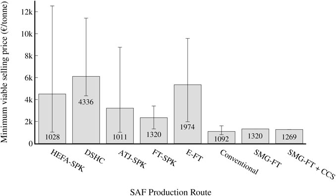
FIGURE 12. MVSP (production cost) taking into account a CO₂ tax of 130 €/tonne of the various SAF cost and emissions benchmarks (see section 3.1) and conventional aviation fuel. The grey bar represents the median cost and emissions found for each process route among studies, while the error bars correspond to the lowest and highest cost and emissions found for each process route. The text states the lowest calculated cost for each SAF production route.

As well as increasing the economic competitiveness of the SMG-FT process, the NPV of the process investment also increases when a CO₂ tax is considered. Using current conventional jet fuel prices with the same 130 €/tonne CO₂ tax applied, the NPV for the standard process increases to 82 M€ while the CCS process increases to 100 M€, and the yearly cash flow turns positive with a payback time of 4.59 years for the standard scenario and 4.22 years for the CCS scenario.

It should also be noted that even though the process significantly reduces emissions from the attached steel mill, and therefore potentially also reducing the cost in CO₂ taxes for the steel mill, none of the saved costs is assumed to be shared in this study. However, it is likely that a SMG-FT producer could be incentivized by sharing the saved costs on CO₂ taxes with the steel mill, which would further reduce the production costs of the SAF. For example, with a CO₂ tax of 130 €/tonne, if 50% of the cost savings from reducing CO₂ emissions at the steel mill was shared with the SMG-FT process, the MVSP for the standard process would be reduced to 1,156 €/tonne, and the CCS process to 1,029 €/tonne, reductions of 164 €/tonne and 240 €/tonne respectively.

5.5 Sensitivity analysis

The sensitivity of both economic indicators (MVSP and NPV) to important and uncertain factors was analysed. Firstly, the behaviour of both indicators for a range of feasible CO₂ tax values was calculated for both the normal and CCS scenario (Figure 13). The MVSP for both SMG-FT scenarios is significantly higher than the conventional price with no CO₂ tax applied, but the MVSP of the conventional scenario rises sharply as the tax increases, compared to a moderate increase for the normal SMG-FT scenario and a slow increase for the SMG-FT CCS scenario. The CCS scenario becomes cheaper than conventional jet fuel at a value of 1,310 €/tonne when a CO₂ tax of about 190 €/tonne is applied, while the normal SMG-FT scenario only becomes cheaper when a CO₂ tax of around 255 €/tonne is in effect. Both scenarios start with negative NPVs; the CCS scenario becomes positive with a CO₂ tax of approximately 208 €/tonne, and the normal scenario with a CO₂ tax of around 290 €/tonne. While the CCS scenario initially has a higher MVSP and lower NPV, it overtakes the normal scenario when a CO₂ tax of around 75 €/tonne is in effect.

FIGURE 13

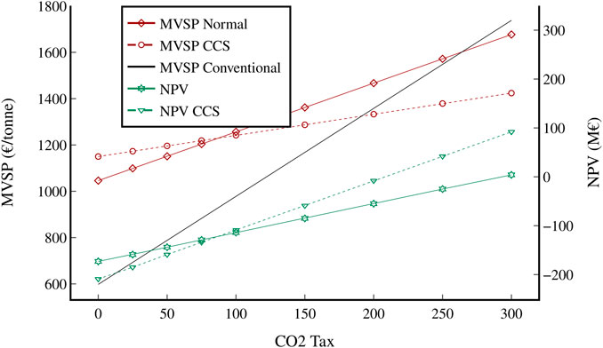
FIGURE 13. Change in MVSP and NPV for both scenarios and the conventional benchmark with respect to the CO₂ emissions tax. All other variables remained constant. The median value of the conventional benchmark was used (2021 average).

The effect of the sales price and discount rate on the NPV was also investigated for both scenarios and is shown in Figure 14. Each variable was adjusted from 50% to 200% of its baseline. The sales price has a much larger impact on the NPV, ranging from −278 M€ for the normal scenario at a sales price of 50% of the median benchmark to an NPV of 36 M€ if the sales price would double. The range of sales prices shown in Figure 14 is also roughly reflective of the range of jet fuel prices from 2020 to 2022, with 2020 having comparatively low prices of 325 €/tonne and 2022 having extremely high prices of 1,087 €/tonne; therefore, changes of this order of magnitude are realistic and greatly affect the economic viability of the SMG-FT process. In comparison, changes in the discount rate do not have as large of an impact, with a discount rate half as high as the baseline resulting in an NPV of -217 M€ for the standard scenario, increasing to −126 M€ if the discount rate doubled. Figure 15.

FIGURE 14

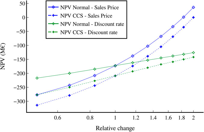
FIGURE 14. Change in NPV for both scenarios with respect to changes in the sales price and discount rate. All other variables remained constant.

FIGURE 15

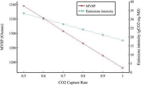
FIGURE 15. Change in MVSP and emissions intensity of the CCS scenario with respect to changes in the CO₂ capture rate. A CO₂ tax of 130 €/tonne was used.

An additional sensitivity analysis was conducted on the CO₂ capture rate from the FT reactors in the CCS scenario. The CO₂ capture rates studied range from 50 to 100%, and a CO₂ tax of 130 €/tonne was assumed. As expected, the emissions intensity of the fuel decreases as the capture rate increases, from an emissions intensity of 33.4 gCO₂-eq./MJ for a capture rate of 50% to 18.1 gCO₂-eq./MJ if all CO₂ was to be captured. The MVSP of the fuel also decreases (1,338 €/tonne at a capture rate of 50% to 1,252 €/tonne at a capture rate of 100%), as the CO₂ tax is greater than the capture cost, making it economical to capture and remove as much CO₂ as possible.

6 Discussion

6.1 Data, model and process analysis

The selected fixed-bed LTFT technology with an iron catalyst is established on an industrial scale and model equations exist (Jess et al., 1999; de Klerk, 2011a). The Aspen and Berkley Madonna simulations show strong accordance with published results, and the simulation results are hence reliable. The model could potentially be improved with the use of two chain-growth factors in the ASF distribution, as opposed to the single factor used in this study. The single factor approach was selected due to the difficulty of connecting an accurate product distribution with an elaborate kinetic model. However, it results in lower than expected C3 and C4 quantities, resulting in a low yield from the alkylation and oligomerisation units. One solution could be to use two separate ASF distributions, one for < C4 components and one for above, though this would significantly increase the calculation effort.

An ideal cracking model is employed in the hydrocracker to calculate the cracking of components longer than C16. The ideal cracking model fits well with experimental results (Weitkamp, 1978; Calemma et al., 2010), but in its current setup the model does not include isomerisation, which is another key task of the hydrocracker. Branched isomers have not been introduced in the simulation since they would considerably raise the required calculation effort and their key property of lowering the jet fuel freeze point can only be confirmed experimentally. Hence, there is no merit in introducing isomerisation to the simulation model. It should, however, be determined whether the methyl branching introduced in a real hydrocracker sufficiently lowers the freezing point of C16 cracking products (below −47°C) for their use in jet fuel.

The aromatisation unit is calculated based on a range of experimental results. While the catalysts used in the experiments differ, this does not affect the result, since the Ga HZSM5 and Ni H-ZSM5 catalysts produce the same product distribution, only with slightly differing conversions (Viswanadham et al., 2004). Nonetheless, all experimental results are derived from small-scale setups and a scale-up to industrial size could alter the heat transfer behaviour, thus changing conversion and selectivity. The inaccuracies of using experimental data could be avoided by employing a rigorous kinetic model (Nguyen et al., 2006). However, it is unnecessary to significantly increase the complexity since only 12% of the jet fuel yield is dependent on the aromatisation reactor, as outlined in section 5.1. Additionally, a more accurate molecular distribution is irrelevant since the mass yield of aromatics is the determining factor. The same applies to the alkylation unit, which is responsible for only 4% of the jet fuel produced in the process.

The complete process calculation is set up as a stationary simulation, which was selected as mass streams, equipment sizes and energy requirements are the main objectives of the study. Stationary simulations use more robust equation systems than dynamic simulations and numerical solving is easier. However, a shortcoming of stationary simulations is that they do not account for process changes over time, compared to a more complex dynamic simulation. The temperature in the FT reactors, aromatization unit, and hydrocracker needs to be increased over time to keep the conversion constant. In addition to the time-dependent conversion change, catalyst regeneration also needs to be considered. In particular, the H-ZSM five catalyst in the aromatisation unit needs to be regenerated in a N₂ atmosphere after only days on stream (de Klerk et al., 2003). This results in downtime for the process, which is taken into account in the 8,000 h/y production time. Nevertheless, with a dynamic simulation there is potential to more accurately model the plant downtime per year.

A major benefit of the SMG-FT process is that it is much more industrially ready than most other SAF production routes (TRL 9). The production and refining of jet fuel using FT synthesis has been operated on a large industrial scale by SASOL for decades (De Klerk, 2010). Additionally, it has been shown that FT synthesis works well with a N₂-rich feedstock stream, as would be the case in the SMG-FT process (Jess et al., 1999). Other SAF routes require further research and development, and perhaps demonstration scale plants, before they can be operated successfully at industrial scale. Therefore, the SMG-FT process is likely to be a more realistic SAF production route in the short term than many other SAF production routes.

Potentially the largest issue with the process is scalability and flexibility, as it must be tied to a steel mill. This makes it hard for economy-of-scale effects to play a big role (Gim and Yoon, 2012), in contrast to other SAFs and conventional jet fuel, which could be built on significantly larger scales. The limiting factor for the size of the plant is the amount of COG produced by the steel mill, as COG contains the H₂ necessary for the FT reaction. This could be supplemented with an electrolysis unit to increase capacity, which would however likely also increase the production cost. The plant must also always be located near a steel mill to ensure easy and cost-effective transport of the steel mill gas, which limits the number of potential spaces to build the technology. Additionally, the technology should be implemented in the short to medium term, as in the long term it is likely that most steel mills will use a low-emissions production method such as renewable H₂, instead of the standard integrated process on which this study is based.

6.2 TEA analysis

The determined MVSP for each scenario is comparable with the lower end of MVSPs found for other SAF routes. Therefore, the process has the economic potential to be a successful SAF production route in the mid-term future. Neither scenario is currently competitive with conventional jet fuel and only becomes economically competitive at a CO₂ price of around 190 €/tonne for the CCS scenario, at which point the CCS scenario has a lower MVSP than the standard scenario due to its decreased emissions intensity. Therefore, it is recommended that the CCS scenario be favoured over the standard scenario, as the extra emission reduction benefits it offers outweigh the CCS cost at higher CO₂ taxes. Naturally, the applicability and cost of CCS will differ greatly depending on the region of the study; some locations will have the potential to store CO₂ close by, whereas others may either require piping of the CO₂ long distances or CCS may be completely unfeasible.

The economic assessment methods used in the study are mature empirical formulas that are standard industry practice. Therefore, the results from the TEA are reasonably certain (±30% inherent error margin using the selected method). It should be noted that the price of conventional jet fuel fluctuates significantly more and at greater magnitudes than the price of SMG-FT. The main variable costs in SMG-FT are the electricity price and the steel mill gas purchase cost (which also depends on the electricity price). Historically, the electricity price has been much more stable than the price of jet fuel, which is heavily dependent on the crude oil price. It is therefore feasible that in periods of high crude oil prices, SMG-FT SAF could become cheaper than conventional jet fuel at an earlier time (or a lower CO₂ price) than previously expected; likewise, if the crude oil price drops significantly, conventional jet fuel could again become the most economical option even after extended periods where SAFs are cheaper to produce. In general, the increased cost stability of SMG-FT is a positive as it would reduce the current volatility of jet fuel prices.

Differing electricity prices by country or region could greatly affect the economic viability of the SMG-FT process. Electricity itself makes up a substantial cost (see Figure 8), but it also affects the purchase cost of the steel mill gases (Collis et al., 2021), which make up the largest overall contribution to OpEx. The purchase cost of COG and BFG is defined by the calorific value they provide to the steel mill in either electricity generation or heat. As most of the electricity generated in this way is sold to the grid, if COG is taken from the steel mill and used to produce SAF, this represents a lost revenue stream for the steel mill that needs to be replaced by the SAF plant, which is effectively the steel mill gas purchase cost. Consequently, if the price of grid electricity is lower in a certain location, not only does it reduce the utility burden on the SMG-FT plant through the electricity it directly consumes, but also by lowering the amount it has to pay the steel mill for the steel mill gases, as they also provide less monetary value to the steel mill. It is therefore recommended that case studies be completed for individual steel mills, as the cost of the steel mill gases could change significantly for different locations. Natural gas prices also have an impact on the steel mill gas price, as the steel mill must replace the heat it obtains from the steel mill gases with natural gas.

A major economic factor is the choice to not separate CO and H₂ from the steel mill gases, but to feed them directly to the FT process. This is essentially a trade-off; as more gas is required to go through the FT reactors, the reactors must be larger and more gas must be compressed (76% of the gas stream entering the FT reactors is inert). Additionally, fewer flash units would be needed throughout the plant and the required CO₂ separation would be reduced. However, the separation of steel mill gases is difficult and expensive, and those initial separation costs are therefore avoided. A thorough study into the separation costs for steel mill gases would help determine which option is more cost-effective.

It would be possible to reduce electricity costs by switching to steam-powered compressors. In a steel mill, large amounts of excess heat are available that could be used to generate steam, which could be compressed and superheated to drive turbines. A detailed process analysis of a steam compression process would be required to determine if it is more economical than the electric compression assumed in this study. Another economic consideration related to process design is the chosen operating pressure for the FT reactors. Compression costs are a major fraction of the overall MVSP, but decreasing the pressure would require an increased reactor size and catalyst mass, as well as affect the reactor conversion. A sensitivity analysis of these factors could optimize the pressure from an economic perspective.

6.3 GHG emissions accounting analysis

The CCS scenario of the SMG-FT process has an emissions intensity comparable to the lowest found SAF benchmarks other than the FT-SPK route, while the standard scenario has emissions similar to the average emissions found for most routes. Both are significantly lower than the emissions intensity of conventional jet fuel. Additionally, the process would reduce the emissions of a steel mill by 130–190 ktCO₂-eq./y. Therefore, the use of steel mill gas to produce SAF has high viability from an emissions reduction perspective. As an LCA is out of the scope of this study and could be the focus of a unique study, a relatively simple GHG emissions calculation was used (see GHG emissions assessment). Therefore, the GHG emission results are more uncertain than the TEA results. However, they can still be used for comparative purposes as the scope of the emissions study is the same as the benchmarks. As the steel mill’s emissions are allocated to steel production, only an analysis of the SAF production process is required, which greatly simplifies the study. As in an LCA, emissions of the feedstocks required were accounted for, as well as emissions generated during the process and combustion of the product. Similarly to the TEA, as the process develops further, the amounts of materials required could change as well, resulting in changes to the process emissions intensity.

The GHG emission calculations are currently carried out under the assumption that electricity is produced in France with an emissions intensity of 67 gCO₂-eq./kWh (Ember, 2021) and that the H₂ for the hydrocracker is produced through natural gas reforming. If both commodities were to originate from renewable sources, a further 15 ktCO₂-eq./y could be saved. In the second FT reactor, a high water content results in large amounts of CO₂ being formed from the water-gas shift reaction. Condensation and subsequent reheating of the large inlet gas stream were dismissed due to the ensuing high capital and operational expenses for two very large heat exchangers. However, it could be worthwhile to analyse this in more detail in an exergy analysis, to find out if more exergy is wasted in the unwanted water-gas-shift reaction or by cooling and reheating the inlet stream. The absence of water in the second reactor has the potential to decrease the annual CO₂ emissions by 28 ktCO₂-eq./y, while at the same time boosting hydrocarbon production by 8 kt/y.

As discussed in section 6.2, different locations and regions have different methods of electricity production, which affects not only the cost but also the emissions intensity of grid electricity. As the process consumes a lot of electricity directly, this could have a large effect on the emissions intensity of the process. As well as the direct electricity usage, the emissions intensity of the steel mill gases depends on the grid electricity emissions intensity as well, as the electricity supplied by the steel mill to the grid will have to be replaced by an increased electricity generation from other power sources. The location for this study was France, but if a SMG-FT plant is to be built in a country with a higher grid emissions intensity, this could drastically increase the process emissions intensity.

It is likely in many scenarios that the SAF plant will be built by a different party than the steel mill. In this case, it is unclear which party can claim the emissions reductions for the purposes of taxes and certificates. Practically speaking, this would be managed on a case-by-case basis between the two parties themselves; likely, one party will legally claim the emissions reductions and the subsidies would be shared according to contracts agreed upon by the parties. As the SMG-FT process is likely to use CCS if possible given location-based restraints, it could also be possible for the steel mill to utilize CCS, as it could share the same infrastructure as the SMG-FT plant. Both the steel mill and the SMG-FT process would then benefit from economy-of-scale effects for the carbon capture process and the steel mill could significantly reduce its emissions.

As mentioned in section 6.2, it is unclear if it would be more cost-effective to separate H₂ and CO from the steel mill gases before they enter the FT reactor. If these gases were separated, resulting in a smaller gas stream, the inclusion of water separation in front of the second FT reactor would be more realistic due to the decreased cost of cooling and reheating the gas stream. This would reduce the CO₂ emissions of the process and increase the product yield.

7 Conclusion

SAF production from steel mill gases is a promising method to produce low-cost and low-emissions aviation fuel that can be substituted for conventional fuel without radical change to aircraft design. A simulation of the process was completed in Aspen Plus and Berkeley Madonna, as well as a TEA and GHG emissions analysis. The MVSP and emissions intensity of the process is compared to both other SAFs and conventional fossil-fuel-based jet fuel to assess its economic and environmental viability. Two scenarios for the studied SMG-FT process were evaluated; one “standard” scenario and one CCS scenario, where the CO₂ emitted from the FT reactors is captured and stored.

The determined MVSP for the process was 1,046 €/tonne for the standard scenario and 1,150 €/tonne for the CCS scenario. These costs are similar overall to the lowest costs found for SAF benchmarks (904 €/tonne for HEFA-SPK, 1,123 €/tonne for CHJ, and 921 €/tonne for ATJ-SPK), and the mean costs for those benchmarks (4,274 €/tonne, 2,065 €/tonne and 3,004 €/tonne respectively) are significantly higher than the calculated MVSP for both SMG-FT scenarios (Yao et al., 2017; Bauen et al., 2020; Dahal et al., 2021). The cost for fossil-fuel-based jet fuel is lower than the MVSP for all SAFs found, although it is highly volatile (ranging from 325 €/tonne to 1,087 €/tonne since January 2020 with a median of 594 €/tonne) (Jet-A1-Fuel, 2020; Jet-A1-Fuel, 2021). It is therefore expected that a CO₂ tax or credit will be needed to make SAFs economically viable, and many SAF TEAs assume such a tax. Investigation of the GHG emissions of the SMG-FT process found that the standard process has an emissions intensity of 49 gCO₂-eq./MJ, while the CCS process has an emissions intensity of 21 gCO₂-eq./MJ. This is similar to other SAF benchmarks, with only the FT-SPK route being significantly lower than the CCS route (lowest found emissions intensity of -3 gCO₂-eq./MJ), and both scenarios are significantly lower than conventional jet fuel, which has an average emissions intensity of 88 gCO₂-eq./MJ. When a CO₂ tax of 130 €/tonne is taken into account, the MVSP for the standard scenario increases to 1,320 €/tonne and the CCS scenario to 1,269 €/tonne. However, the price for conventional jet fuel increases to 797–1,604 €/tonne, which makes the SMG-FT process much more competitive with conventional jet fuel.

Overall, the process offers a SAF production method that is cost competitive with the lowest-cost SAFs and with comparable GHG emissions savings. It is expected to be economically viable with a CO₂ tax of around 190 €/tonne. The main drawbacks of the process include a lack of scalability in comparison to conventional jet fuel, as it is limited in size by the steel mill, as well as uncertain viability in the long term if steel mills switch away from the integrated BF-BOF process. Needed further studies include a full LCA on the process to better clarify the GHG emissions intensity of the fuel, and case studies on individual steel mills.

Data availability statement

The original contributions presented in the study are included in the article/Supplementary Material, further inquiries can be directed to the corresponding author.

Author contributions

KD performed literature analysis, developed the model and performed the techno-economic assessment. JC supervised the study, further developed the techno-economic assessment and emissions analysis and was the author of all text. All authors read, commented, developed structure, and approved the final manuscript.

Funding

This research was carried out within the project Carbon4PUR, which received funding from the European Union’s Horizon 2020 research and innovation program under grant agreement no. 825999. The European Commission is neither responsible nor liable for the content of this document.

Conflict of interest

The authors declare that the research was conducted in the absence of any commercial or financial relationships that could be construed as a potential conflict of interest.

Publisher’s note

All claims expressed in this article are solely those of the authors and do not necessarily represent those of their affiliated organizations, or those of the publisher, the editors and the reviewers. Any product that may be evaluated in this article, or claim that may be made by its manufacturer, is not guaranteed or endorsed by the publisher.

Supplementary material

The Supplementary Material for this article can be found online at: https://www.frontiersin.org/articles/10.3389/fenrg.2022.1049229/full#supplementary-material

References

Abanades, J. C., Rubin, E. S., Mazzotti, M., and Herzog, H. J. (2017). On the climate change mitigation potential of CO2 conversion to fuels. Energy Environ. Sci. 10, 2491–2499. doi:10.1039/c7ee02819a

CrossRef Full Text | Google Scholar

Agarwal, A. K., and Valera, H. (2022). Introduction of greener and scalable E-fuels for decarbonization of transport. Energy, environment, and sustainability. Berlin, Germany: Springer. doi:10.1007/978-981-16-8344-2_1

CrossRef Full Text | Google Scholar

Albuquerque, J. S., Costa, F. O., and Barbosa, B. V. S. (2019). Fischer-Tropsch synthesis: Analysis of products by anderson-schulz-flory distribution using promoted cobalt catalyst. Catal. Lett. 3, 831–839. doi:10.1007/s10562-019-02655-4

CrossRef Full Text | Google Scholar

Alexander, B., Shashank, S., William Leif, F., Madalsa, S., and Venkatasubramanian, V. (2020). Performance metrics required of next- generation batteries to electrify commercial aircraft. ACS Energy Lett. 5, 663–668. doi:10.1021/acsenergylett.9b02574

CrossRef Full Text | Google Scholar

Arens, M., Worrell, E., Eichhammer, W., Hasanbeigi, A., and Zhang, Q. (2017). Pathways to a low-carbon iron and steel industry in the medium-term – The case of Germany. J. Clean. Prod. 163, 84–98. doi:10.1016/j.jclepro.2015.12.097

CrossRef Full Text | Google Scholar

Artz, J., Muller, T. E., Thenert, K., Kleinekorte, J., Meys, R., Sternberg, A., et al. (2018). Sustainable conversion of carbon dioxide: An integrated review of catalysis and life cycle assessment. Chem. Rev. 118, 434–504. doi:10.1021/acs.chemrev.7b00435

PubMed Abstract | CrossRef Full Text | Google Scholar

Ausfelder, F., and Wagemann, K. (2020). Power-to-Fuels: E-Fuels as an important option for a climate-friendly mobility of the future. Chem. Ing. Tech. 92, 21–30. doi:10.1002/cite.201900180

CrossRef Full Text | Google Scholar

Baral, N. R., Kavvada, O., Mendez-Perez, D., Mukhopadhyay, A., Lee, T. S., Simmons, B. A., et al. (2019). Techno-economic analysis and life-cycle greenhouse gas mitigation cost of five routes to bio-jet fuel blendstocks. Energy Environ. Sci. 12, 807–824. doi:10.1039/c8ee03266a

CrossRef Full Text | Google Scholar

Bauen, A., Bitossi, N. N., German, L., Harris, A., and Leow, K. (2020). Sustainable Aviation Fuels: Status, challenges and prospects of drop-in liquid fuels, hydrogen and electrification in aviation. Johns. Matthey Technol. Rev. 62, 234–299. doi:10.1595/205651320x15816756012040

CrossRef Full Text | Google Scholar

Bellevrat, E., and Menanteau, P. (2009). Introducing carbon constraint in the steel sector: ULCOS scenarios and economic modeling. Rev. Mater. Paris. 106, 318–324. doi:10.1051/metal/2009059

CrossRef Full Text | Google Scholar

Börse (2022). Naphtha historisch. Available at: https://www.boerse-online.de/rohstoffe/historisch/naphthapreis/eur/1.1.2021_31.12.2021. (Accessed August 24, 2022)

Google Scholar

Bouchy, C., Hastoy, G., Guillon, E., and Martens, J. A. (2009). Fischer-Tropsch waxes upgrading via hydrocracking and selective hydroisomerization. Oil Gas Sci. Technol. - Rev. IFP. 64, 91–112. doi:10.2516/ogst/2008047

CrossRef Full Text | Google Scholar

Broker, G. (2022). Platinum price. Available at: https://www.goldbroker.com/charts/platinum-price/eur. (Accessed June 27, 2022)

Google Scholar

Buchner, G. A., Zimmermann, A. W., Hohgräve, A. E., and Schomäcker, R. (2018). Techno-economic assessment framework for the chemical industry—based on technology readiness levels. Ind. Eng. Chem. Res. 57, 8502–8517. doi:10.1021/acs.iecr.8b01248

CrossRef Full Text | Google Scholar

Budsberg, E., Crawford, J. T., Morgan, H., Chin, W. S., Bura, R., and Gustafson, R. (2016). Hydrocarbon bio-jet fuel from bioconversion of poplar biomass: Life cycle assessment. Biotechnol. Biofuels 9, 1–13. doi:10.1186/s13068-016-0582-2

PubMed Abstract | CrossRef Full Text | Google Scholar

Calemma, V., Peratello, S., Pavoni, S., Clerici, G., and Perego, C. (2001). Hydroconversion of a mixture of long chain n-paraffins to middle distillate: Effect of the operating parameters and products properties. Stud. Surf. Sci. Catal. 136, 307–312. doi:10.1016/s0167-2991(01)80321-9

CrossRef Full Text | Google Scholar

Calemma, V., Gambaro, C., Parker, W. O., Carbone, R., Giardino, R., and Scorletti, P. (2010). Middle distillates from hydrocracking of FT waxes: Composition, characteristics and emission properties. Catal. Today 149, 40–46. doi:10.1016/j.cattod.2009.03.018

CrossRef Full Text | Google Scholar

California Air Resources Board (2020). Low carbon fuel standard regulation. Available at https://www.sciencedirect.com/topics/engineering/low-carbon-fuel-standard. (Accessed June 27, 2022)

Google Scholar

Collis, J., and Schomäcker, R. (2022). Determining the production and transport cost for H2 on a global scale. Front. Energy Res. 10. 909298. doi:10.3389/fenrg.2022.909298

CrossRef Full Text | Google Scholar

Collis, J., Strunge, T., Steubing, B., Zimmermann, A., and Schomäcker, R. (2021). Deriving economic potential and GHG emissions of steel mill gas for chemical industry. Front. Energy Res. 9, 1–22. doi:10.3389/fenrg.2021.642162

CrossRef Full Text | Google Scholar

Commercial Aviation Alternative Fuels Initiative (CAAFI) (2021). Fuel qualification. CAAFI. Available at https://www.caafi.org/focus_areas/fuel_qualification.html. (Accessed May 04, 2022)

Google Scholar

Dahal, K., Brynolf, S., Xisto, C., Hansson, J., Grahn, M., Gronstedt, T., et al. (2021). Techno-economic review of alternative fuels and propulsion systems for the aviation sector. Renew. Sustain. Energy Rev. 151, 111564. doi:10.1016/j.rser.2021.111564

CrossRef Full Text | Google Scholar

Damodaran, A. (2019). Cost of capital by sector. Available at https://pages.stern.nyu.edu/∼adamodar/New_Home_Page/datafile/wacc.htm. (Accessed May 18, 2022)

Google Scholar

De Jong, S., Antonissen, K., Hoefnagels, R., Lonza, L., Wang, M., Faaij, A., et al. (2017). Life-cycle analysis of greenhouse gas emissions from renewable jet fuel production. Biotechnol. Biofuels 10, 64–18. doi:10.1186/s13068-017-0739-7

PubMed Abstract | CrossRef Full Text | Google Scholar

de Klerk, A. (2009). Can Fischer-Tropsch syncrude be refined to on-specification diesel fuel? Energy fuels. 23, 4593–4604. doi:10.1021/ef9005884

CrossRef Full Text | Google Scholar

de Klerk, A. (2003). “Deactivation behaviour of Zn/ZSM-5 with a fischer-tropsch derived feedstock,” in Catalysis in application. Editors J. Hargreaves, D. Lennon, and D. Jackson (London, UK: Royal Society of Chemistry), 24–31.

Google Scholar

De Klerk, A. (2010). Fischer-Tropsch jet fuel process. Patent number.: US20100108568A1. Available at: https://www.sciencedirect.com/topics/engineering/fischer-tropsch-process. (Accessed April 10, 2022)

Google Scholar

de Klerk, A. (2011). Fischer-tropsch refining. Weinheim, Germany: Wiley VCH.

Google Scholar

de Klerk, A. (2011). Fischer–Tropsch fuels refinery design. Energy Environ. Sci. 4, 1177–1205. doi:10.1039/c0ee00692k

CrossRef Full Text | Google Scholar

de Klerk, A. (2008). Fischer–Tropsch refining: Technology selection to match molecules. Green Chem. 10, 1249–1279. doi:10.1039/b813233j

CrossRef Full Text | Google Scholar

Dry, M. E. (1981). Data on arge catalyst. Catal. Sci. Technol. 1, 159–255.

Google Scholar

Ember (2021). Data explorer. Available at: https://ember-climate.org/data/data-explorer/. (Accessed August 11, 2022)

Google Scholar

Epstein, A., and O’Flarity, S. (2019). Considerations for reducing aviation’s CO2 with aircraft electric propulsion. J. Propuls. Power 35, 572–582. doi:10.2514/1.b37015

CrossRef Full Text | Google Scholar

Eswaran, S., Subramaniam, S., Geleynse, S., Brandt, K., Wolcott, M., and Zhang, X. (2021). Techno-economic analysis of catalytic hydrothermolysis pathway for jet fuel production. Renew. Sustain. Energy Rev. 151, 111516. doi:10.1016/j.rser.2021.111516

CrossRef Full Text | Google Scholar

EUROFER (2019). Pathways to a CO2-neutral European steel industry. Brussels: EUROFER.

Google Scholar

Fagerström, A., Grahn, D., Lundberg, S., Ghosh, S., Creaser, D., Olsson, L., et al. (2021). Large scale bio electro jet fuel production integration at CHP-plant in Östersund. Sweden: Swedish environmental research institute. Available at: https://www.ivl.se/download/18.2f05652c1775c6085c01a6/1612270805586/B2407.pdf.

Google Scholar

Farooq, D., Thompson, I., and Ng, K. S. (2020). Exploring the feasibility of producing sustainable aviation fuel in the UK using hydrothermal liquefaction technology: A comprehensive techno-economic and environmental assessment. Clean. Eng. Technol. 1, 100010. doi:10.1016/j.clet.2020.100010

CrossRef Full Text | Google Scholar

Fischedick, M., Marzinkowski, J., Winzer, P., and Weigel, M. (2014). Techno-economic evaluation of innovative steel production technologies. J. Clean. Prod. 84, 563–580. doi:10.1016/j.jclepro.2014.05.063

CrossRef Full Text | Google Scholar

Fortier, M. O. P., Roberts, G. W., Stagg-Williams, S. M., and Sturm, B. S. M. (2014). Life cycle assessment of bio-jet fuel from hydrothermal liquefaction of microalgae. Appl. Energy 122, 73–82. doi:10.1016/j.apenergy.2014.01.077

CrossRef Full Text | Google Scholar

Gabrielli, P., Gazzani, M., and Mazzotti, M. (2020). The role of carbon capture and utilization, carbon capture and storage, and biomass to enable a net-zero-CO2 emissions chemical industry. Ind. Eng. Chem. Res. 59, 7033–7045. doi:10.1021/acs.iecr.9b06579

CrossRef Full Text | Google Scholar

Garrett, D. E. (2012). Chemical engineering economics. Berlin, Germany: Springer Netherlands.

Google Scholar

Gim, B., and Yoon, W. L. (2012). Analysis of the economy of scale and estimation of the future hydrogen production costs at on-site hydrogen refueling stations in Korea. Int. J. Hydrogen Energy 37, 19138–19145. doi:10.1016/j.ijhydene.2012.09.163

CrossRef Full Text | Google Scholar

Glenk, G., and Reichelstein, S. (2019). Economics of converting renewable power to hydrogen. Nat. Energy 4, 216–222. doi:10.1038/s41560-019-0326-1

CrossRef Full Text | Google Scholar

Gössling, S., Humpe, A., Fichert, F., and Creutzig, F. (2021). COVID-19 and pathways to low-carbon airtransport until 2050. Environ. Res. Lett. 16, 034063. doi:10.1088/1748-9326/abe90b

CrossRef Full Text | Google Scholar

Gray, N., Mcdonagh, S., Shea, R. O., Smyth, B., and Murphy, J. D. (2021). Decarbonising ships , planes and trucks: An analysis of suitable low-carbon fuels for the maritime, aviation and haulage sectors. Adv. Appl. Energy 1, 100008. doi:10.1016/j.adapen.2021.100008

CrossRef Full Text | Google Scholar

Hanaoka, T., Miyazawa, T., Shimura, K., and Hirata, S. (2015). Jet fuel synthesis in hydrocracking of Fischer-Tropsch product over Pt-Loaded zeolite catalysts prepared using microemulsions. Fuel Process. Technol. 129, 139–146. doi:10.1016/j.fuproc.2014.09.011

CrossRef Full Text | Google Scholar

Hannula, I., Kaisalo, N., and Simell, P. (2020). Preparation of synthesis gas from CO2 for fischer–tropsch synthesis—comparison of alternative process configurations. C–J. of Car. Res. 6, 55. doi:10.3390/c6030055

CrossRef Full Text | Google Scholar

Hasanbeigi, A., Arens, M., and Price, L. (2014). Alternative emerging ironmaking technologies for energy-efficiency and carbon dioxide emissions reduction: A technical review. Renew. Sustain. Energy Rev. 33, 645–658. doi:10.1016/j.rser.2014.02.031

CrossRef Full Text | Google Scholar

He, K., and Wang, L. (2017). A review of energy use and energy-efficient technologies for the iron and steel industry. Renew. Sustain. Energy Rev. 70, 1022–1039. doi:10.1016/j.rser.2016.12.007

CrossRef Full Text | Google Scholar

Hemmings, B., Calvo Ambel, C., Buffet, L., Gilliam, L., and Sihvonen, J. (2018). Roadmap to decarbonising European aviationBrussels: Transport and Environment.

Google Scholar

Hillestad, M. (2015). Modeling the fischer–tropsch product distribution and model implementation. Chem. Prod. Process Model. 10, 147–159. doi:10.1515/cppm-2014-0031

CrossRef Full Text | Google Scholar

Hoogendoorn, J. C. (1975). New applications of the Fischer-Tropsch process. Clean Fuels Coal Symposium II, 343–358.

Google Scholar

Huq, N. A., Hafenstine, G. R., Huo, X., Nguyen, H., Tifft, S. M., Conklin, D. R., et al. (2021). Toward net-zero sustainable aviation fuel with wet waste–derived volatile fatty acids. Proc. Natl. Acad. Sci. U. S. A. 118, e2023008118. doi:10.1073/pnas.2023008118

PubMed Abstract | CrossRef Full Text | Google Scholar

IATA (2021). Fact Sheet: EU and US policy approaches to advance SAF production. Montreal, Canada: IATA.

Google Scholar

IATA (2018). Forecast predicts 8.2 billion air travelers in 2037. Montreal, Canada: IATA. Press release no. 62 Available at: https://www.iata.org/en/pressroom/pr/2018-10-24-02/.

Google Scholar

IATA (2022). Fuel price monitor. Montreal, Canada: International air transport association. Available at https://www.iata.org/en/publications/economics/fuel-monitor/.

Google Scholar

IEA (2019). Are aviation biofuels ready for take off? Available at https://www.iea.org/commentaries/are-aviation-biofuels-ready-for-take-off. (Accessed March 27, 2022)

Google Scholar

Im-orb, K., Simasatitkul, L., and Arpornwichanop, A. (2015). Performance analysis and optimization of the biomass gasification and fischer-tropsch integrated process for green fuel productions. Comput. Aided Chem. Eng. 37, 275–280. doi:10.1016/B978-0-444-63578-5.50041-4

CrossRef Full Text | Google Scholar

IRENA (2016). Innovation Technology outlook for advanced liquid biofuels. Int. Renew. Energy Agency 132.

Google Scholar

IPCC (2022). Climate change 2022 - impacts, adapation and vulnerability. Geneva, Switzerland: IPCC.

Google Scholar

Jess, A., and Kern, C. (2009). Modeling of multi-tubular reactors for Fischer-Tropsch synthesis. Chem. Eng. Technol. 32, 1164–1175. doi:10.1002/ceat.200900131

CrossRef Full Text | Google Scholar

Jess, A., Popp, R., and Hedden, K. (1999). Fischer–Tropsch-synthesis with nitrogen-rich syngas: Fundamentals and reactor design aspects. Appl. Catal. A General 186, 321–342. doi:10.1016/s0926-860x(99)00152-0

CrossRef Full Text | Google Scholar

Jess, A., and Wasserscheid, P. (2013). Chemical technology : An integral textbook. Weinheim, Germany: Wiley VCH.

Google Scholar

Jet-A1-Fuel (2018). Average jet a1 price 2018 = 85$ per bbl. Jet-A1-Fuel. Available at: https://jet-a1-fuel.com/average/2018. (Accessed May 19, 2022)

Google Scholar

Jet-A1-Fuel (2019). Average jet a1 price 2019 = 79$ per bbl. Jet-A1-Fuel. Available at: https://jet-a1-fuel.com/average/2019. (Accessed May 19, 2022)

Google Scholar

Jet-A1-Fuel (2020). Average jet a1 price 2020 = 46$ per bbl. Jet-A1-Fuel. Available at: https://jet-a1-fuel.com/average/2020. (Accessed May 19, 2022)

Google Scholar

Jet-A1-Fuel (2021). Average jet a1 price 2021 = 78$ per bbl. Jet-A1-Fuel. Available at: https://jet-a1-fuel.com/average/2021. (Accessed May 19, 2022)

Google Scholar

Kheshgi, H. S. S., Thomann, H., Bhore, N. A., Hirsch, R. B., Parker, M. E., and Teletzke, G. F. (2012). Perspectives on CCS cost and economics. SPE Econ. Manag. 4, 24–31. doi:10.2118/139716-pa

CrossRef Full Text | Google Scholar

KLM (2022). KLM further expands approach for Sustainable Aviation Fuel, Haarlemmermeer, Netherlands: KLM. Available at: https://news.klm.com/klm-further-expands-approach-for-sustainable-aviation-fuel/.

Google Scholar

Krishnamurthy, V., and Viswanathan, V. (2020). Beyond transition metal oxide cathodes for electric aviation: The case of rechargeable CF_x. ACS Energy Lett. 5, 3330–3335. doi:10.1021/acsenergylett.0c01815

CrossRef Full Text | Google Scholar

Kuntze, T., Hedden, K., and Jess, A. (1995). From natural gas to liquid hydrocarbons (3): Kinetics of the Fischer-Tropsch-synthesis using a nitrogen-rich synthesis gas. Erdöl, Erdgas, Kohle 111, 67–71.

Google Scholar

Lai, Y. Y., Karakaya, E., and Björklund, A. (2022). Employing a socio-technical system Approach in prospective life cycle assessment : A case of large-scale Swedish sustainable aviation fuels. Front. Sustain. 3, 1–20. doi:10.3389/frsus.2022.912676

CrossRef Full Text | Google Scholar

Liu, R., Zhu, H. q., Wu, Z. w., Qin, Z. f., Fan, W. b., and Wang, J. g. (2015). Aromatization of propane over Ga-modified ZSM-5 catalysts. J. Fuel Chem. Technol. 43, 961–969. doi:10.1016/s1872-5813(15)30027-x

CrossRef Full Text | Google Scholar

Lufthansa (2022). Sustainable aviation fuel - lufthansa group. Available at https://www.lufthansagroup.com/en/themes/sustainable-aviation-fuel.html (Accessed March 28, 2022)

Google Scholar

Ma, W., Jacobs, G., Sparks, D. E., Todic, B., Bukur, D. B., and Davis, B. H. (2020). Quantitative comparison of iron and cobalt based catalysts for the Fischer-Tropsch synthesis under clean and poisoning conditions. Catal. Today 343, 125–136. doi:10.1016/j.cattod.2019.04.011

CrossRef Full Text | Google Scholar

Malicier, V. (2022). Fuel suppliers urge governments to impose SAF blending mandates. London, UK: S&P Global Commodity Insights. Available at: https://www.spglobal.com/commodityinsights/en/market-insights/latest-news/oil/111121-fuel-suppliers-urge-governments-to-impose-saf-blending-mandates.

Google Scholar

Marchese, M., Giglio, E., Santarelli, M., and Lanzini, A. (2020). Energy performance of Power-to-Liquid applications integrating biogas upgrading, reverse water gas shift, solid oxide electrolysis and Fischer-Tropsch technologies. Energy Convers. Manag. X 6, 100041. doi:10.1016/j.ecmx.2020.100041

CrossRef Full Text | Google Scholar

Marcoline, F. V., Furth, J., Nayak, S., Grabe, M., and Macey, R. I. (2022). Berkeley Madonna Version 10–A simulation package for solving mathematical models. CPT. Pharmacometrics Syst. Pharmacol. 11, 290–301. doi:10.1002/psp4.12757

PubMed Abstract | CrossRef Full Text | Google Scholar

Martinez-Hernandez, E., Ramírez-Verduzco, L. F., Amezcua-Allieri, M. A., and Aburto, J. (2019). Process simulation and techno-economic analysis of bio-jet fuel and green diesel production — minimum selling prices. Chem. Eng. Res. Des. 146, 60–70. doi:10.1016/j.cherd.2019.03.042

CrossRef Full Text | Google Scholar

Mashapa, T. N., and de Klerk, A. (2007). Solid phosphoric acid catalysed conversion of oxygenate containing Fischer–Tropsch naphtha. Appl. Catal. A General 332, 200–208. doi:10.1016/j.apcata.2007.08.001

CrossRef Full Text | Google Scholar

Mazumdar, D., and Evans, J. W. (2009). Modeling of steelmaking processes. Florida, USA: CRC Press.

Google Scholar

Ministry of Defence Uk (2011). Defence standard 91-91 issue 7 A2. Def. Stand., 91.

Google Scholar

Ministere de l’Économie et des Finances (2017). Ministere de l’Économie et des Finances: Les 4 pages de la direction générale desentreprises (DGE): France’s manufacturing sector has improved its price competitivenessbut non-price competitiveness still needs attention. techreport.

Google Scholar

Moretti, C., Vera, I., Junginger, M., López-Contreras, A., and Shen, L. (2022). Attributional and consequential LCAs of a novel bio-jet fuel from Dutch potato by-products. Sci. Total Environ. 813, 152505. doi:10.1016/j.scitotenv.2021.152505

PubMed Abstract | CrossRef Full Text | Google Scholar

Mousavi-Avval, S. H., and Shah, A. (2021). Techno-economic analysis of hydroprocessed renewable jet fuel production from pennycress oilseed. Renew. Sustain. Energy Rev. 149, 111340. doi:10.1016/j.rser.2021.111340

CrossRef Full Text | Google Scholar

Naims, H. (2016). Economics of carbon dioxide capture and utilization—A supply and demand perspective. Environ. Sci. Pollut. Res. 23, 22226–22241. doi:10.1007/s11356-016-6810-2

PubMed Abstract | CrossRef Full Text | Google Scholar

Nguyen, L. H., Vazhnova, T., Kolaczkowski, S. T., and Lukyanov, D. B. (2006). Combined experimental and kinetic modelling studies of the pathways of propane and n-butane aromatization over H-ZSM-5 catalyst. Chem. Eng. Sci. 61, 5881–5894. doi:10.1016/j.ces.2006.05.017

CrossRef Full Text | Google Scholar

Panja, P., McPherson, B., and Deo, M. (2022). Techno-economic analysis of amine-based CO2 capture technology: Hunter plant case study. Carbon Capture Sci. Technol. 3, 100041. doi:10.1016/j.ccst.2022.100041

CrossRef Full Text | Google Scholar

Peters, R., Wegener, N., Samsun, R. C., Schorn, F., Riese, J., Grunewald, M., et al. (2022). A techno-economic assessment of fischer – tropsch fuels based on syngas from Co-electrolysis. Processes 699, 699. doi:10.3390/pr10040699

CrossRef Full Text | Google Scholar

Pietzcker, R. C., Osorio, S., and Rodrigues, R. (2021). Tightening EU ETS targets in line with the European Green Deal: Impacts on the decarbonization of the EU power sector. Appl. Energy 293, 116914. doi:10.1016/j.apenergy.2021.116914

CrossRef Full Text | Google Scholar

PWC (2016). Comparison of electricity and gas prices for large industrial consumers. London, United Kingdom: PWC.

Google Scholar

Raak, H., and Hedden, K. (1998). A pressurized reactor with integrated load cell for measuring the activities of Fischer-Tropsch-Catalysts and their loadings with liquid reaction products (Wax); Druckreaktor mit Waegezelle zur Messung der Aktivitaet und Wachsbeladung von Fischer-Tropsch-. Erdöl, Erdgas, Kohle 114, 251–256.

Google Scholar

Ramirez, A., Sarathy, S. M., and Gascon, J. (2020). CO2 derived E-fuels: Research trends, misconceptions, and future directions. Trends Chem. 2, 785–795. doi:10.1016/j.trechm.2020.07.005

CrossRef Full Text | Google Scholar

Rogelj, J. (2018). Mitigation pathways compatible with 1.5°C in the context of sustainable development. Geneva, Switzerland: Intergovernmental Panel on Climate Change. Available at: https://www.ipcc.ch/site/assets/uploads/sites/2/2019/02/SR15_Chapter2_Low_Res.pdf.

Google Scholar

Scheelhaase, J., Maertens, S., and Grimme, W. (2019). Synthetic fuels in aviation - current barriers and potential political measures. Transp. Res. Procedia 43, 21–30. doi:10.1016/j.trpro.2019.12.015

CrossRef Full Text | Google Scholar

Sakuneka, T. M., De Klerk, A., Nel, R. J. J., and Pienaar, A. D. (2008). Synthetic jet fuel production by combined propene oligomerization and aromatic alkylation over solid phosphoric acid. Ind. Eng. Chem. Res. 47, 1828–1834. doi:10.1021/ie0710566

CrossRef Full Text | Google Scholar

Seeley, B. A., Seeley, D., and Rakas, J. (2020). A report on the future of electric aviation, doi:10.7922/G2BC3WTVAvailable at: https://escholarship.org/uc/item/4t76186k.

CrossRef Full Text | Google Scholar

Sekiguchi, N., Otsuka, H., de Carvalho, A., and Silfa, F. (2015). Capacity developments in the World steel industry. Available at: https://www.oecd.org/industry/ind/Capacity-Developments-Steel-Industry.pdf%0Ahttps://www.oecd.org/sti/ind/Capacity-Developments-Steel-Industry.pdf. (Accessed March 28, 2022)

Google Scholar

Sheehan, J. J. (2009). Biofuels and the conundrum of sustainability. Curr. Opin. Biotechnol. 20, 318–324. doi:10.1016/j.copbio.2009.05.010

PubMed Abstract | CrossRef Full Text | Google Scholar

Song, C., Liu, S., Li, X., Xie, S., Liu, Z., and Xu, L. (2014). Influence of reaction conditions on the aromatization of cofeeding n-butane with methanol over the Zn loaded ZSM-5/ZSM-11 zeolite catalyst. Fuel Process. Technol. 126, 60–65. doi:10.1016/j.fuproc.2014.04.018

CrossRef Full Text | Google Scholar

Sun, C., Zhan, T., Pfeifer, P., and Dittmeyer, R. (2017). Influence of Fischer-Tropsch synthesis (FTS) and hydrocracking (HC) conditions on the product distribution of an integrated FTS-HC process. Chem. Eng. J. 310, 272–281. doi:10.1016/j.cej.2016.10.118

CrossRef Full Text | Google Scholar

Sun, H., Luo, Z., Li, S., Xue, S., and Zhou, Q., (2021). Comparative life cycle assessment (LCA) of biofuel production via corn stover: Fermentation to ethanol, pyrolysis to bio-oil, and gasification to jet fuel. Biomass Convers. Biorefinery 1, 3. doi:10.1007/s13399-021-02054-z

CrossRef Full Text | Google Scholar

Suresh, P., Malina, R., Staples, M. D., Lizin, S., Olcay, H., Blazy, D., et al. (2018). Life cycle greenhouse gas emissions and costs of production of diesel and jet fuel from municipal solid waste. Environ. Sci. Technol. 52 (21), 12055–12065. doi:10.1021/acs.est.7b04277

PubMed Abstract | CrossRef Full Text | Google Scholar

Tongpun, P., Wang, W.-C., and Srinophakun, P. (2019). Techno-economic analysis of renewable aviation fuel production: From farming to refinery processes. J. Clean. Prod. 226, 6–17. doi:10.1016/j.jclepro.2019.04.014

CrossRef Full Text | Google Scholar

Towler, G., and Sinnott, R. (2017). Chemical engineering Principles, practice and economics of plant and process design. Amsterdam, Netherlands: Elsevier.

Google Scholar

Trippe, F., Frohling, M., Schultmann, F., Stahl, R., Henrich, E., and Dalai, A. (2013). Comprehensive techno-economic assessment of dimethyl ether (DME) synthesis and Fischer–Tropsch synthesis as alternative process steps within biomass-to-liquid production. Fuel Process. Technol. 106, 577–586. doi:10.1016/j.fuproc.2012.09.029

CrossRef Full Text | Google Scholar

Tsupari, E., Karki, J., Arasto, A., Lilja, J., Kinnunen, K., and Sihvonen, M. (2015). Oxygen blast furnace with CO2 capture and storage at an integrated steel mill – Part II: Economic feasibility in comparison with conventional blast furnace highlighting sensitivities. Int. J. Greenh. Gas Control 32, 189–196. doi:10.1016/j.ijggc.2014.11.007

CrossRef Full Text | Google Scholar

Turton, R., Bailie, R. C., Whiting, W. B., and Shaeiwitz, J. A. (2008). Analysis, synthesis and design of chemical processes. London, UK: Pearson Education.

Google Scholar

Turton, R., and Shaeiwitz, J. (2017). Chemical process equipment design. New York: Pearson.

Google Scholar

Ueckerdt, F., Bauer, C., Dirnaichner, A., Everall, J., Sacchi, R., and Luderer, G. (2021). Potential and risks of hydrogen-based e-fuels in climate change mitigation. Nat. Clim. Chang. 11, 384–393. doi:10.1038/s41558-021-01032-7

CrossRef Full Text | Google Scholar

Uribe-Soto, W., Portha, J. F., Commenge, J. M., and Falk, L. (2017). A review of thermochemical processes and technologies to use steelworks off-gases. Renew. Sustain. Energy Rev. 74, 809–823. doi:10.1016/j.rser.2017.03.008

CrossRef Full Text | Google Scholar

van de Loosdrecht, J., Botes, F. G., Ciobica, L. M., Gibson, P., Weststrate, C. J., Botes, F. G., et al. (2013). in 7.20 - fischer–tropsch synthesis: Catalysts and chemistry (Amsterdam, Netherlands: Elsevier), 525–557. doi:10.1016/B978-0-08-097774-4.00729-4

CrossRef Full Text | Google Scholar

Viswanadham, N., Muralidhar, G., and Rao, T. S. R. P. (2004). Cracking and aromatization properties of some metal modified ZSM-5 catalysts for light alkane conversions. J. Mol. Catal. A Chem. 223, 269–274. doi:10.1016/j.molcata.2003.11.045

CrossRef Full Text | Google Scholar

Wang, W.-C. (2016). Techno-economic analysis of a bio-refinery process for producing Hydro-processed Renewable Jet fuel from Jatropha. Renew. Energy 95, 63–73. doi:10.1016/j.renene.2016.03.107

CrossRef Full Text | Google Scholar

Wei, W., Yang, W., Hultgren, A., Mellin, P., Wang, C., and Salman, H. (2013). Utilization of biomass for blast furnace in Sweden. Sweden: kth royal institute of technology.

Google Scholar

Weitkamp, J. (1978). Hydrocracking, cracking and isomerization of hydrocarbons. Erdöl, Erdgas, Kohle 31, 13–22.

Google Scholar

World Steel Association (2020). Steel’s contribution to a low-carbon future and climate resilient societies. Brussels, Belgium: World Steel Association. Available at: http://www.worldsteel.org/dms/internetDocumentList/bookshop/Steel-s-Contribution-to-a-Low-Carbon-Future-/document/Steel’s-Contribution-to-a-Low-Carbon-Future.pdf.

Google Scholar

World Steel Association (2020). World Steel Association. Belgium: World Steel Association. Available at http://www.worldsteel.org/wsif.php.World steel in figures

Google Scholar

Yao, G., Staples, M. D., Malina, R., and Tyner, W. E. (2017). Stochastic techno-economic analysis of alcohol-to-jet fuel production. Biotechnol. Biofuels 10, 18–13. doi:10.1186/s13068-017-0702-7

PubMed Abstract | CrossRef Full Text | Google Scholar

Yoo, E., Lee, U., and Wang, M. (2022). Life-cycle greenhouse gas emissions of sustainable aviation fuel through a net-zero carbon biofuel plant design. ACS Sustain. Chem. Eng. 10, 8725–8732. doi:10.1021/acssuschemeng.2c00977

CrossRef Full Text | Google Scholar

Zauba, Zauba. Available at https://www.zauba.com/. (Accessed August 11, 2022)

Google Scholar

Zimmermann, A. W., Marxen, A., Buchner, G. A., Katelhon, A., Sternberg, A., Naims, H., et al. (2020). Techno-economic assessment & life cycle assessment guidelines for CO2 utilization. Ann Arbor, Michigan: University of Michigan Library. doi:10.3998/2027.42/162573

CrossRef Full Text | Google Scholar

Nomenclature

Abbreviations

ATJ Alcohol-to-jet

BFG Blast furnace gas

BOFG Basic oxygen furnace gas

CapEx Capital expenditure

CHJ Catalytic hydrothermolysis jet

COG Coke oven gas

DSHC Direct sugar to hydrocarbons

FT Fischer-Tropsch

GHG Greenhouse gas

HDCJ Hydro-processed depolymerized cellulosic jet

HEFA Hydroprocessed esters and fatty acids

HTFT High-temperature Fischer Tropsch

HTL Hydrothermal liquefaction

LCA Life-cycle assessment

LHHW Langmuir–Hinshelwood Hougen-Watson

LTFT Low-temperature Fischer Tropsch

MVSP Minimum viable selling price

NPV Net present value

OpEx Operational expenditure

SAF Sustainable aviation fuel

SMG Steel mill gas

SPK Synthetic paraffinic kerosene

TEA Techno-economic assessment.