A two-stage deep learning framework for early-stage lifetime prediction for lithium-ion batteries with consideration of features from multiple cycles

1 Introduction

Nowadays, lithium-ion batteries are utilized in a wide range of applications, from portable devices to grid-level energy storage, due to their high energy density, high power density, long lifetime, and falling cost (Chen T. et al., 2021; Severson et al., 2019). However, a long battery lifetime impedes battery development because it takes months or years to observe the deterioration. Moreover, despite the standardized manufacturing processes of lithium-ion batteries, even from the same batch, batteries can have significantly different lifetime due to internal heterogeneity (porosity, thickness, and etc.) and different operation conditions. Therefore, early-stage lifetime prediction methods are crucial to assess batteries in advance and shorten the required experimental time which can accelerate battery research, production, and design optimization (Chen B. R. et al., 2021).

Existing studies for battery lifetime prediction can generally be divided into two groups: model-based methods and data-driven methods. For the model-based methods, researchers either start with an empirical model with explicit parameters (Schmalstieg et al., 2014) or a model (equivalent circuit model or electrochemical model) combined with advanced filtering algorithms to estimate the aging status (He et al., 2011; Arachchige et al., 2017; Wassiliadis et al., 2018). Xing et al. (2013) used a particle filter to update the parameters within an empirical exponential and a polynomial regression model to track the battery’s degradation trend. With a simple battery model, Saha et al. (2009) proposed a particle filter method to predict the state of charge (SOC), state of health (SOH), and remaining useful life (RUL) based on the correlations between the battery capacity and resistance. Yang et al. (2019) implemented a particle filter with a semi-empirical model based on Coulombic efficiency, which is highly correlated with the loss of active lithium inventory, to estimate the battery health. To facilitate the resample process within the particle filter. Tang et al. (2019) proposed a model-oriented gradient-correction particle filter method for future degradation. By using the base-model as a regulation within the evolution of the particle, the global information from the base model is utilized and help the model achieve a better prediction result. Gao et al. (2022) proposed a SOC and SOH co-estimated framework comprising a simplified electrochemical model and dual nonlinear filter. Compared with the mathematical model, which is not adaptive to the real-time behavior of the battery, the filter-based prediction approach treats parameters as state variables that are identified online with real-time data. Therefore, compared with empirical models, filter methods offer better precision and accuracy. However, they still have some drawbacks: 1) the performance is greatly affected by the underlying battery degradation model; 2) early-cycle prediction remains a challenge for these methods because of limited capacity lost in the early cycles (Fei et al., 2022).

Unlike model-based methods, statistical and machine learning approaches can infer from the cycle data and offer a more general approach to predict battery lifetime in the early stage stages of operation. Moreover, statistical and machine learning approaches are attractive, with the recent improvement in algorithms and computational power, and the growing availability of battery cycling data. Nowadays, many studies have been done using these advanced methods to address engineering problems, such as computational fluid dynamics, molecular design, and so on (Reich, 1997; Liakos et al., 2018; Sanchez-Lengeling and Aspuru-Guzik, 2018; Brunton et al., 2020; Hegde and Rokseth, 2020; Mendez, 2022). Nonetheless, these techniques are also applied in predicting battery lifetime. With the extracted features, previous capacity trend, temperature and depth of discharge, and so on. Liu et al. (2019) predicted cyclic aging using Gaussian progress regression (GPR) with a modified kernel which reflects the electrochemical behavior. To further improve the model performance, instead of using features to construct a regression model alone, a base model is firstly fitted to learn the battery’s long life information, and then a migrated mean function and migrated-GPR model are used to predict the fading curve with 30% starting data (Liu et al., 2022). Besides GPR (Richardson et al., 2017; 2019b; 2019a), the recurrent neural network (RNN), especially the long short-term memory (LSTM) network (Zhang et al., 2018; Gupta et al., 2021; Hu et al., 2021, 2022; Li et al., 2021; Uddin et al., 2022), is usually used in battery fading curve prediction due to its extraordinary ability in handling time-series data. Zhang et al. (2018) used the LSTM network to synthesize a data-driven battery RUL predictor. The drop-out method is applied to avoid overfitting, and the Monte Carlo (MC) simulation is used to generate the RUL prediction uncertainties. Furthermore, to utilize the advantage of the LSTM network and GPR. Liu et al. (2021) decompose the capacity data with the empirical mode decomposition (EMD) method and feed the decomposed result to LSTM and GPR, respectively. Therefore, the long-term dependency of capacity is captured by the LSTM network, while the uncertainty quantification caused by the capacity regeneration is captured by the GPR. Other methods such as deep neural network (Hsu et al., 2022), linear regression with elastic net (Severson et al., 2019), random forest (Yang et al., 2022), stacked denoising autoencoders (Xu et al., 2021), etc., are used to predict RUL or to extrapolate battery fading curve with some starting cycle data.

Early-stage lifetime prediction with limited data is crucial for battery development and deployment and remains a challenge for researchers. During the early stage, batteries will undergo a formation process in which the electrochemical behavior is different than in operation after the early stage. For example, many batteries’ capacity increases in the early stage which is a behavior that has not been fully understood yet (Guo et al., 2022). This behavior results in relatively small capacity changes during the early stage. Therefore, predicting lifetime with early cycle data is challenging. Existing methods generally require 40%–70% of historical data of the entire battery lifetime to estimate the model parameters or train a data-driven model (Hu et al., 2020). Therefore, careful feature engineering is needed to generate features that highly correlate with lifetime while given limited cycle data.

Feature engineering is a necessary process of selecting, manipulating, and transforming raw data into features that can be used in model development. Proper feature engineering can ease the modeling difficulty and enable the model to output results of higher quality (Zheng and Casari, 2018). Generally, features for battery prognosis can be derived from 1) raw data (voltage/current/temperature-time curve); 2) incremental capacity and differential voltage analysis; 3) directly measured variables; 4) statistical metrics; and 5) extraction from a deep neural network with raw data input (Fei et al., 2022). These features are extracted through two feature extraction techniques: 1) traditional knowledge-guided feature extraction and 2) deep learning based automatic feature extraction. The traditional method ensures that the extracted features are relevant to the lifetime prediction and have physical meaning and implication. For example, temperature is often used. The physical meaning behind this feature is that as batteries lose capacity, the internal resistance increases, resulting in a higher temperature during operation. In contrast to the physics-knowledge-guided feature extraction, using a deep neural network to extract features is hard to understand and lacks physical meaning due to the black-box nature of the neural network. Nevertheless, extracting features from time-series data, especially physics-guided features, has seldom been studied. Fei et al. (2022) construct the features from 2nd, 10th, and 100th cycle. To represent the features’ evolution curve, Paulson et aluse three multi-cycle features to capture the median, derivative with respect to cycles (Paulson et al., 2022). Attia et al. (2021) extract the feature from the difference between 10th and 100th cycle along with fourteen summary statistic functions and four feature transformations. However, the aging process is a continuous process, and information can be extracted from the development trend of physics-guided features. Instead of using some statistic metric to keep track of the changes in features, Greenbank et alutilize the distribution of the features within a certain time and use the value at a certain percentile as input features (Greenbank and Howey, 2022). Furthermore, by treating the capacity-voltage curves from multiple cycles as a picture, Saxena et al. (2022) use a convolution neural network to extract three parameters for the proposed capacity fading curve model.

Combining physics-guided and deep learning-based automatic feature extraction methods, in this study, we proposed a novel two-stage data-driven feature engineering framework for predicting battery lifetime with early-stage cycle data. In the first stage, with physics-guided insight, features are extracted from the first 100 cycles of data to form time series data that contain information from each cycle and how the features evolve during battery aging. Next, a gated recurrent unit (GRU)-based autoencoder is used to process and extract information from the time series data and eliminate the time domain. Finally, an elastic net regression model is used to build a regression model between extracted features and battery lifetime.

2 Battery dataset

In this study, the dataset is provided by the Massachusetts Institute of Technology (Severson et al., 2019), which is the largest known dataset for studying the degradation behavior of lithium-ion batteries. This dataset contains 124 lithium iron phosphate (LFP) batteries with different charging policies. However, within this dataset, there is an outlier with a lifetime less than 300 cycles. Therefore, the outlier is removed to avoid further problems in the following study. The batteries are cycled until losing 20% of their nominal capacity (1.1 Ah), which is a standard end-of-life criterion for the battery industry. Due to various operation conditions, the lifetime ranges from 300 to 2300 cycles, as shown in Figure 1.

FIGURE 1

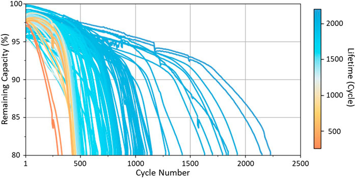
FIGURE 1. Battery capacity fade curves of the dataset. The lifetime ranges from 300 to 2300 cycles.

3 A two-stage data-driven feature engineering framework

In this section, the proposed two-stage data-driven feature engineering framework is introduced. The framework is depicted in Figure 2, which is comprised of extracting physics-guided features from early-stage raw data, a GRU-based autoencoder, feature selection, and lifetime regression. First of all, with physical knowledge, five features are selected and calculated within multiple cycles to form a time series dataset. Then, the time series dataset is compressed with the GRU-based autoencoder to remove the time domain. A feature selection is applied to the compressed features to increase the performance of final regression models. Finally, the selected features are used to train and test the regression model.

FIGURE 2

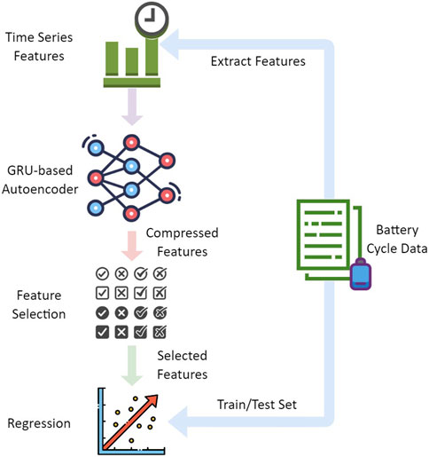
FIGURE 2. The two-stage data-driven feature engineering framework for the early-stage battery lifetime prediction.

3.1 Physics-guided features

During cycling, due to electrochemical reactions such as the SEI formation and lithium plating, lithium-ion batteries will gradually lose capacity. In this study, five features are selected.

1) Log variance of the difference of the discharge curve between two cycles (ln var ΔQ_N-10). The physical meaning behind this features is related to the dependence of the discharged energy dissipated in voltage (Severson et al., 2019). Generally, for an aged battery, due to loss of capacity, the discharge curve will shift lower, as demonstrated in Figure 3A.

2) Log minimum of the difference of the discharge curve between two cycles (ln min ΔQ_N-10). In contrast to the previous feature, which uses variance to capture the difference between two designed curves, Feature 2 focuses on the local difference, indicating the largest difference between the two cycles.

3) The internal resistance (IR) difference between two cycles (ln ΔIR_N-4). The formation process is crucial for the operation of Li-ion batteries. A successful formation of SEI can help to minimize solvent reduction and graphite exfoliation. The capacity retention and storage life of the Li-ion batteries directly depend on the stability of the SEI. However, during the early stage, due to trapped air within the electrode, part of the electrode is not soaked with electrolyte leading to high internal resistance (Jeon, 2019). As the formation process progresses, the trapped air will be consumed, forming the SEI layer and reducing the internal resistance. Therefore, as shown in Figure 3B, the IR drops in the few beginning cycles. However, as the trapped gas diminishes, the SEI formation behavior becomes dominant, along with the loss of active lithium-ion inventory and the loss of active electrode material. All these aging behaviors increase internal resistance in later cycles (Figure 3B). Therefore, by measuring the difference in the internal resistance between the two cycles, we can extrapolate how the aging behavior will happen in the future and predict the corresponding lifetime.

4) Difference of the maximum temperature between two cycles (ΔTmax _N-10). Corresponding to Feature 3, as the internal resistance increase, during charging and discharging, more heat is generated (Figure 3C). The maximum temperature difference between two cycles infers the internal degradation status.

5) Log variance of the temperature difference during discharge (ln var ΔT_N-10). Unlike Feature 4, this feature focuses more on the temperature difference during discharging. Moreover, as shown in Figure 3D, the temperature is plotted against voltage, which can help capture changes in temperature and voltage curves.

FIGURE 3

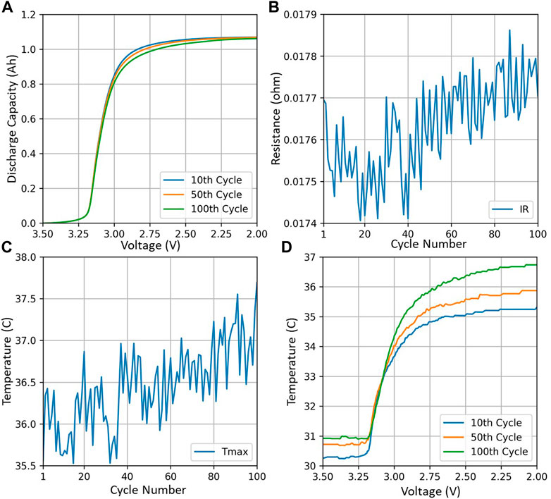
FIGURE 3. Different feature behaviors for battery #b2c33. (A) Discharge Capacity vs. discharge voltage at different cycles; (B) Internal resistance trend; (C) Maximum temperature trend; (D) Discharge temperature vs. discharge voltage at different cycles.

In contrast to previous studies, in which features are only extracted from some specific cycles, this study calculates features from multiple cycles (cycle 11–100) and forms a time series dataset, $X\in R^{m\times 90\times 5}$, where m is the number of batteries. So far, guided by electrochemical knowledge, five features are extracted from 90 cycles. However, ignoring the time domain and using all these features to build a regression model may lead to an overfitting issue because the number of features (90 × 5 = 450) is far more than the number of samples. Moreover, battery aging is a continuous process, and some information is hidden within the time series. Therefore, in the next stage, a GRU-based autoencoder is applied to compress the time series dataset, extract hidden information, and eliminate the time domain.

3.2 GRU based autoencoder

To address the need to handle time series data, an RNN is proposed. Unlike the traditional neural network and convolutional neural network, the hidden input within the RNN contains hidden information from previous input. Therefore, the RNN considers not only the current input but also the previous input. But RNNs, in general, face a short-term memory issue due to the vanishing gradient problem. To address this issue, LSTM and GRU are proposed and able to handle the long-time series problem by introducing the forgetting mechanism. Compared with LSTM, which has already been used to predict fading curves (Zhang et al., 2018; Hu et al., 2021; Li et al., 2021), the GRU has a simple structure. Therefore, it usually converges faster than LSTM and fits well, given a small dataset. Moreover, the GRU has similar performance compared to LSTM. Thus, in this study, the GRU is chosen to build the autoencoder. The structure of GRU is shown in Figure 4. The inputs are processed with Eqs 1–4 (Cho et al., 2014). The GRU comprises a reset gate and an update gate. The reset gate controls how much previous information needs to be forgotten by a sigmoid function which range from 0 to 1. In this application, the reset gate can help to reduce the noise or measure error from the time series data and obtain better features. On the other hand, the update gate determine how much of the past information needs to be passed along to the next state. Note that the subscript t represents the moment which means the cycle that features are extracted. The superscripts are used to distinguish different variables. h denotes the hidden state, x represents the input, W is the matrix of weight, b is the bias. Variables are in vector form.

$\mathrm{R}\mathrm{e}\mathrm{s}\mathrm{t}\mathrm{G}\mathrm{a}\mathrm{t}\mathrm{e}:r_t=\sigma \left(W^1{h}_{t-1}+U^1{x}_t+b^1\right)(1)$

$\mathrm{U}\mathrm{p}\mathrm{d}\mathrm{a}\mathrm{t}\mathrm{e}\mathrm{G}\mathrm{a}\mathrm{t}\mathrm{e}:z_t=\sigma \left(W^2{h}_{t-1}+U^2{x}_t+b^2\right)(2)$

$h_t^{\prime }=\tanh \left(W^3{x}_t+r_t{U}^3{h}_{t-1}\right)(3)$

$h_t=z_t{h}_t^{\prime }+\left(1-z_t\right)h_{t-1}(4)$

FIGURE 4

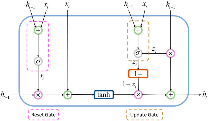
FIGURE 4. GRU structure.

Thanks to the electrochemical knowledge-guided feature selection, there is a strong relationship between the time series data and the battery lifetime. However, treating time series data as individual features will lead to model information redundancy and computational inefficiency. For example, in our case, if we treat time series data from every cycle as an individual feature, there will be 450 features (5 × 90). For modeling, the information dimension is related to the information representation ability. However, an increasing number of dimensions often result in model information redundancy and overfitting caused by the increasing number of correlated features. Specifically, in our case, the features extracted from cycle N+1 may contain most of the information from cycle N. Therefore, it is necessary to reduce the number of dimensions to improve model performance. Currently, many methods have been proposed to reduce dimension, such as principal component analysis (PCA), independent component analysis (ICA), and the autoencoder method. However, both PCA and ICA are applicable due to the lack of Gaussian distribution and prior knowledge. Therefore, an autoencoder is utilized.

In contrast to other artificial neural networks, by introducing a bottleneck structure, the neural network can be divided into two multi-layer neural networks, denoted as the encoder and the decoder. Both neural networks are trained simultaneously. During training, the encoder learns a compressed representation of the data while the decoder learns how to recover information from the compressed representation. The quality of the compressed information is evaluated by calculating the mean square error between the recovered data and the original data. In this study, the autoencoder is trained with mini-batch and stochastic gradient descent.

3.3 Feature analysis

Feature analysis is carried out to analyze the correlation between the compressed features obtained from the GRU-based autoencoder and the target battery lifetime. The correlation is evaluated with the Pearson correlation coefficient, which ranges from −1 (negative correlation) to 1 (positive correlation), as defined in Eq. 5. M denotes the total number of batteries. $j$ denotes compressed feature $j$. $x_{ij}$ represents values of feature j for battery $i$. ${\overline{x}}_j$ denotes the average value of feature $j$. $y_i$ is the lifetime of battery $i$. $\overline{y}$ is the average lifetime of the sample set.

$r_j=\frac{{\displaystyle \sum }_{\mathit{i}=1}^{\mathit{m}}\left({\mathit{x}}_{\mathit{i}\mathit{j}}-{\overline{\mathit{x}}}_{\mathit{j}}\right)\left({\mathit{y}}_{\mathit{i}}-\overline{\mathit{y}}\right)}{\sqrt{{\displaystyle \sum }_{\mathit{i}=1}^{\mathit{m}}{\left({\mathit{x}}_{\mathit{i}\mathit{j}}-{\overline{\mathit{x}}}_{\mathit{j}}\right)}^2}\sqrt{{\displaystyle \sum }_{\mathit{i}=1}^{\mathit{m}}{\left({\mathit{y}}_{\mathit{i}}-\overline{\mathit{y}}\right)}^2}}(5)$

With Eq. 5, the correlation between compressed features and battery lifetime is demonstrated in Figure 5. To avoid interference between each selected features, all features are compressed separately. In other words, five GRU-based autoencoders are trained. Each time series are compressed into three features. For example, compressed feature 1, 2, and 3 are obtained by compressing the time series of ln var ΔQ_N-10. These compressed features contain the most important information within the time series dataset. Therefore, all the compressed features exhibit some correlation with the battery lifetime. Especially compressed feature 1 to 6. These six compressed features are generated by compressing the time series data of ln var ΔQ_N-10 and ln min ΔQ_N-10. Compared with the original time series dataset, in which correlation with battery lifetime fluctuates and varies between cycle and cycle, the compressed features have a relatively stable correlation. This high correlation indicates that the GRU-based autoencoder can capture the most critical information from the time series dataset and reduce the dimension, facilitating the following regression step and elevating the regression model’s performance.

FIGURE 5

FIGURE 5. The Pearson correlation coefficient of the compressed features.

3.4 Feature selection

After the GRU-based autoencoder, the time series dataset is compressed to the features set, $Xc\in R^{m\times 15}$. However, these features may contain some common information with each other. Moreover, feature selection can improve learning performance, increase computational efficiency, and build a better generalization model. There are different kinds of feature selection methods. This study uses the wrapper method as a feature selection method due to its simplicity (Pudil et al., 1994).

3.5 Regression model

With the compressed and selected features, a regression model can be trained to predict the battery lifetime. Different kinds of regression models can be applied to this data set. In this study, three regression models are studied: 1) GPR, 2) support vector regression (SVR), and 3) elastic net.

3.5.1 Gaussian process regression

Derived from the Bayesian framework, GPR has been widely applied to different problems, including the estimation of SOH because of its advantage in flexibility, being nonparametric, being probabilistic, and having good performance with a small dataset (Li et al., 2019). Instead of fitting the training set with some optimal parameter, the GPR assumes the prediction follows a joint Gaussian distribution described by its mean Eq. 6 and covariance Eq. 7. In Eq. 6, y_k is the expected lifetime for battery k, f(x_k) is the distribution of the predicted lifetime, x_k is the features of battery k. In Eq. 7, x' represents the features from the training set. In this study, the well-studied and widely used radial basis function kernel is utilized. The length scale, l, is a hyperparameter and is optimized during validation.

$y_k=E\left(f\left(x_k\right)\right)(6)$

$K\left(x_k,x^{\prime }\right)=\exp \left(\frac{{\Vert x_k-x^{\prime }\Vert }^2}{2l^2}\right)(7)$

3.5.2 Support vector regression

Similar to GPR, SVR is also a nonparametric regression method. Therefore, SVR can be flexible and model any complex system given sufficient data and a proper kernel. Unlike GPR, which uses a kernel to generate the prediction distribution, in SVR, the kernel is used to help to solve the nonlinear problem by transforming data to a higher dimension space where the problem can be solved linearly. SVR is solved by searching for a minimum margin fit for all the input datasets. The SVR problem is demonstrated in Eq. 8.

$\underset{w,b,{\zeta ,\zeta }^{*}}{\min }\frac{1}{2}{w}^{T}w+C{\sum }_{i=1}^N\left({\zeta }_i+{\zeta }_i^{*}\right)$

$\mathrm{s}\mathrm{u}\mathrm{b}\mathrm{j}\mathrm{e}\mathrm{c}\mathrm{t}\mathrm{t}\mathrm{o}{y}_i-w^T\varphi \left(x_i\right)-b\le ϵ+{\zeta }_i^{*}(8)$

$w^T\varphi \left(x_i\right)+b-y_i\le ϵ+{\zeta }_i^{*}$

${\zeta }_i,{\zeta }_i^{*}\ge 0,\forall i$

where $y_i$ is the lifetime for battery $i$, $x_i$ represents the corresponding features, $w$ represents the parameters, b is the bias, C is the regularization parameter, ${\zeta }_i$ and ${\zeta }_i^{*}$ are the slack variables that account for how far the prediction is away from the actual value, and $ϵ$ is the tolerance which allows the model to ignore some noise and helps to generate a general model. $\varphi$ is the function that helps to transfer the dataset into a higher dimension and is defined by the kernel function. In general, instead of solving Eq. 8 directly, the dual problem is solved. In this study, the radial basis function kernel is adopted.

3.5.3 Elastic net regression

Unlike the previous two methods, by introducing l1 and l2 regularization within the objective function Eq. 9, the model can automatically choose the proper features that provide the best regression result. Therefore, in this study, the compressed features, $X\in R^{m\times 15}$, are fed directly into the elastic net regression.

$\underset{w}{\min }\frac{1}{2N}{\left|\left|y-Xw\right|\right|}_2^2+\alpha r_{l1}{\left|\left|w\right|\right|}_1+\frac{1}{2}\alpha \left(1-r_{l1}\right){\left|\left|w\right|\right|}_2^2(9)$

where $y_i$ is the lifetime for battery i, x_i represents the corresponding features, $w$ represents the weight for features, $\alpha$ is the regularization parameter, $r_{l1}$ is the ratio of l1 regularization. Both $\alpha$ and $r_{l1}$ are hyperparameters and optimized with cross-validation during training.

4 Result

In this section, the result of different regression models is presented. To demonstrate the improvement, the proposed framework is compared with a state-of-art regression model (Severson et al., 2019).

In this study, the batteries are randomly separated into a training set (83 batteries) and a testing set (40 batteries). Moreover, for a regression model that requires tuning of hyperparameters, 10-fold cross-validation is applied. The performance of the proposed framework is evaluated with two metrics calculated with Eqs 10 and 11.

Root-mean-square error (RMSE)

$\mathrm{R}\mathrm{M}\mathrm{S}\mathrm{E}=\sqrt{\frac{1}{N}{\displaystyle \sum }_{i=1}^N{\left(y_i-\widehat{y_i}\right)}^2}(10)$

Mean absolute percentage error (MAPE)

$\mathrm{M}\mathrm{A}\mathrm{P}\mathrm{E}=\frac{1}{N}{\displaystyle \sum }_{i=1}^N\frac{\left|y_i-\widehat{y_i}\right|}{y_i}\times 100\%(11)$

where N is the number of batteries, $y_i$ is the actual lifetime of battery i, and $\widehat{y_i}$ is the corresponding predicted lifetime. RMSE represents the absolute error, while MAPE evaluates the relative error. Lower RMSE and MAPE mean smaller prediction error.

4.1 Feature selection performance

Through the GRU-based autoencoder, the original time series dataset, $X\in R^{m\times 90\times 5}$, is compressed to $Xc\in R^{m\times 15}$. However, because of the black-box property of the neural network, these 15 features may contain similar information. Therefore, a feature selection is necessary to produce a regression model that has better performance. To control the impact of different regression models, all selected features are input into a general linear regression model defined as Eq. 12.

$\widehat{Y}=w^T{X}_s+b(12)$

where $\widehat{Y}$ is the vector for predicted lifetime, $X_s$ is the selected features dataset, b is the bias.

A forward wrapper method starts fitting the model with each individual feature one at a time and selects the feature that provides the best prediction result. In step 2, the algorithm will try to fit with two features by trying combinations of the previously selected feature. Step 3 selects the second feature that provides the best prediction result along with previously selected features. Repeat Step 2 and 3 until the number of selected features reaches the desired number. The result is demonstrated in Figure 6. According to the result, in the beginning, as the number of features increases, the test error decreases. This indicates that the regression model gets more information from the additional features. However, after selecting 12 features, adding more features decreases the model performance and increases the test error. This indicates that adding more features causes an overfitting problem due to the shared information within the features. Compared with selecting all 15 features, according to the result, selecting 12 features reduces the test MAPE by about 7 cycles and test MAPE by about 0.32%. Therefore, in the following study, these selected 12 features are used as the input features for the regression model.

FIGURE 6

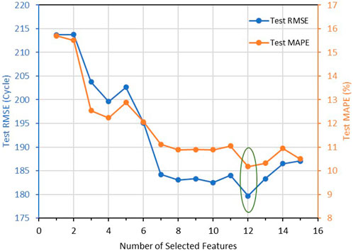
FIGURE 6. Test error (RMSE and MAPE) changes with different selected features. Selecting 12 features provides the best regression result.

According to the result shown in Table 1, the elastic net and GPR provide a similar result. The GPR has a test RMSE at 188.40 cycles and a test MAPE at 10.50%. The elastic net has a test RMSE of 187.99 and a test MAPE of 10.14%. The elastic net has a slightly better performance than GPR. This improvement is caused by the regularization within the elastic net, which will automatically scale down the unimportant features. However, SVR provides a poor performance which may cause by the noise within the dataset. Therefore, the result generated from the elastic net is used in the following comparison.

TABLE 1

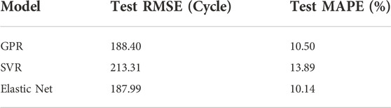
TABLE 1. Metric for different regression models.

To demonstrate the advantage of the proposed framework which utilizes time series dataset, a comparison between the proposed framework and a state-of-art battery lifetime prediction model (discharge model) (Severson et al., 2019) is presented (Figure 7). With the same training set and test set, the benchmark model only uses data from cycle 10 and 100 to construct the necessary features. With the limited information within the selected features, the benchmark only achieves a test RMSE at 209.53 cycles and a test MAPE at 14.17%. Moreover, according to Figure 7, both models tend to under-predict the lifetime for batteries that have a long lifetime (>1500 cycles). This prediction error is caused by the imbalanced sample. In this dataset, there are 116 batteries have a lifetime shorter than 1500 cycles, and only 8 batteries have a lifetime longer than 1500 cycles. Nevertheless, the proposed two-stage feature engineering framework lowers the test RMSE by 10.22% and reduces the test MAPE by 28.44%. This improvement indicates that the proposed framework can recover some information from features obtained from multiple cycles. Furthermore, with the help of the GRU-based autoencoder, the hidden information within the features evolution curve can be recovered and facilitates the lifetime regression model to achieve a better result.

FIGURE 7

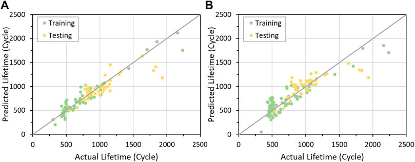
FIGURE 7. The actual lifetime vs. predicted lifetime: (A) Elastic Net; (B) Benchmark.

5 Conclusion

This study proposes a novel two-stage data-driven feature engineering framework to predict battery lifetime with early-stage cycle data. In the first stage, instead of constructing features from certain cycles (Fei et al., 2022; Severson et al., 2019; Paulson et al., 2022), the proposed framework acquires features from multiple cycles, forming a time series dataset. In the second stage, a GRU-based autoencoder is applied to compress the time-series dataset to reduce the features’ dimensionality and recover hidden information within the time domain. After compression, a wrapper method is employed to select the best combination of compressed features to enhance the regression model’s performance. With the selected features, the elastic net model provides the best regression result with a test RMSE at 187.99 and a test MAPE at 10.14%. Furthermore, a comparison with a state-of-art battery lifetime prediction model is presented to demonstrate the proposed framework’s advantage. Compared with the benchmark model, the proposed method lowers the test RMSE by 10.22% and reduces the test MAPE by 28.44%. This work provides insight into extracting information from features obtained from multiple cycles and highlights the information within the features’ evolution curve. By treating the dataset as time series data and compressing it with a GRU-based autoencoder, hidden information can be extracted. In the future, we would like to explore a hybrid model technique that combines both machine learning and physics knowledge.

Data availability statement

Publicly available datasets were analyzed in this study. This data can be found here: https://data.matr.io/1/projects/5c48dd2bc625d700019f3204.

Author contributions

All authors contributed to the concept design and development. JY contributes to the model building, analysis and prepares the draft. All authors contributed to manuscript revision, read, and approved the submitted version.

Conflict of interest

The authors declare that the research was conducted in the absence of any commercial or financial relationships that could be construed as a potential conflict of interest.

Publisher’s note

All claims expressed in this article are solely those of the authors and do not necessarily represent those of their affiliated organizations, or those of the publisher, the editors and the reviewers. Any product that may be evaluated in this article, or claim that may be made by its manufacturer, is not guaranteed or endorsed by the publisher.

References

Arachchige, B., Perinpanayagam, S., and Jaras, R. (2017). Enhanced prognostic model for lithium ion batteries based on particle filter state transition model modification. Appl. Sci. (Basel). 7, 1172. doi:10.3390/APP7111172

CrossRef Full Text | Google Scholar

Attia, P. M., Severson, K. A., and Witmer, J. D. (2021). Statistical learning for accurate and interpretable battery lifetime prediction. J. Electrochem. Soc. 168, 090547. doi:10.1149/1945-7111/AC2704

CrossRef Full Text | Google Scholar

Brunton, S. L., Noack, B. R., and Koumoutsakos, P. (2020). Machine learning for fluid mechanics. Annu. Rev. Fluid Mech. 52, 477–508. doi:10.1146/annurev-fluid-010719-060214

CrossRef Full Text | Google Scholar

Chen, T., Song, M., Hui, H., and Long, H. (2021b). Battery electrode mass loading prognostics and analysis for lithium-ion battery--based energy storage systems. Front. Energy Res. 9, 754317. doi:10.3389/fenrg.2021.754317

CrossRef Full Text | Google Scholar

Chen, B. R., Kunz, M. R., Tanim, T. R., and Dufek, E. J. (2021a). A machine learning framework for early detection of lithium plating combining multiple physics-based electrochemical signatures. Cell Rep. Phys. Sci. 2, 100352. doi:10.1016/j.xcrp.2021.100352

CrossRef Full Text | Google Scholar

Cho, K., Van Merriënboer, B., Bahdanau, D., and Bengio, Y. (2014). On the properties of neural machine translation: Encoder-decoder approaches. Priprint 1409.1259. doi:10.48550/arXiv.1409.1259

CrossRef Full Text | Google Scholar

Fei, Z., Zhang, Z., Yang, F., Tsui, K. L., and Li, L. (2022). Early-stage lifetime prediction for lithium-ion batteries: A deep learning framework jointly considering machine-learned and handcrafted data features. J. Energy Storage 52, 104936. doi:10.1016/J.EST.2022.104936

CrossRef Full Text | Google Scholar

Gao, Y., Liu, K., Zhu, C., Zhang, X., and Zhang, D. (2022). Co-estimation of state-of-charge and state-of- health for lithium-ion batteries using an enhanced electrochemical model. IEEE Trans. Ind. Electron. 69, 2684–2696. doi:10.1109/TIE.2021.3066946

CrossRef Full Text | Google Scholar

Greenbank, S., and Howey, D. (2022). Automated feature extraction and selection for data-driven models of rapid battery capacity fade and end of life. IEEE Trans. Ind. Inf. 18, 2965–2973. doi:10.1109/TII.2021.3106593

CrossRef Full Text | Google Scholar

Guo, J., Li, Y., Meng, J., Pedersen, K., Gurevich, L., and Stroe, D. I. (2022). Understanding the mechanism of capacity increase during early cycling of commercial NMC/graphite lithium-ion batteries. J. Energy Chem. 74, 34–44. doi:10.1016/J.JECHEM.2022.07.005

CrossRef Full Text | Google Scholar

Gupta, A., Sheikh, M., Tripathy, Y., and Widanage, W. D. (2021). Transfer learning LSTM model for battery useful capacity fade prediction. Proceedings of the 2021 24th International Conference on Mechatronics Technology (ICMT) 18-22 Dec. 2021. Singapore. doi:10.1109/ICMT53429.2021.9687230

CrossRef Full Text | Google Scholar

He, W., Williard, N., Osterman, M., and Pecht, M. (2011). Prognostics of lithium-ion batteries based on Dempster–Shafer theory and the Bayesian Monte Carlo method. J. Power Sources 196, 10314–10321. doi:10.1016/J.JPOWSOUR.2011.08.040

CrossRef Full Text | Google Scholar

Hegde, J., and Rokseth, B. (2020). Applications of machine learning methods for engineering risk assessment – a review. Saf. Sci. 122, 104492. doi:10.1016/J.SSCI.2019.09.015

CrossRef Full Text | Google Scholar

Hsu, C. W., Xiong, R., Chen, N. Y., Li, J., and Tsou, N. T. (2022). Deep neural network battery life and voltage prediction by using data of one cycle only. Appl. Energy 306, 118134. doi:10.1016/j.apenergy.2021.118134

CrossRef Full Text | Google Scholar

Hu, T., Ma, H., Liu, K., and Sun, H. (2022). Lithium-ion battery calendar health prognostics based on knowledge-data-driven attention. IEEE Trans. Ind. Electron. 70, 407–417. doi:10.1109/TIE.2022.3148743

CrossRef Full Text | Google Scholar

Hu, X., Xu, L., Lin, X., and Pecht, M. (2020). Battery lifetime prognostics. Joule 4, 310–346. doi:10.1016/J.JOULE.2019.11.018

CrossRef Full Text | Google Scholar

Hu, X., Yang, X., Feng, F., Liu, K., and Lin, X. (2021). A particle filter and long short-term memory fusion technique for lithium-ion battery remaining useful life prediction. J. Dyn. Syst. Meas. Control 143. 4049234. doi:10.1115/1.4049234

CrossRef Full Text | Google Scholar

Jeon, D. H. (2019). Wettability in electrodes and its impact on the performance of lithium-ion batteries. Energy Storage Mat. 18, 139–147. doi:10.1016/J.ENSM.2019.01.002

CrossRef Full Text | Google Scholar

Li, W., Sengupta, N., Dechent, P., Howey, D., Annaswamy, A., and Sauer, D. U. (2021). Online capacity estimation of lithium-ion batteries with deep long short-term memory networks. J. Power Sources 482, 228863. doi:10.1016/J.JPOWSOUR.2020.228863

CrossRef Full Text | Google Scholar

Li, Y., Liu, K., Foley, A. M., Zülke, A., Berecibar, M., Nanini-Maury, E., et al. (2019). Data-driven health estimation and lifetime prediction of lithium-ion batteries: A review. Renew. Sustain. energy Rev. 113, 109254. doi:10.1016/j.rser.2019.109254

CrossRef Full Text | Google Scholar

Liakos, K. G., Busato, P., Moshou, D., Pearson, S., and Bochtis, D. (2018). Machine learning in agriculture: A review. Sensors 18, 2674. doi:10.3390/S18082674

PubMed Abstract | CrossRef Full Text | Google Scholar

Liu, K., Hu, X., Wei, Z., Li, Y., and Jiang, Y. (2019). Modified Gaussian process regression models for cyclic capacity prediction of lithium-ion batteries. IEEE Trans. Transp. Electrific. 5, 1225–1236. doi:10.1109/TTE.2019.2944802

CrossRef Full Text | Google Scholar

Liu, K., Shang, Y., Ouyang, Q., and Widanage, W. D. (2021). A data-driven approach with uncertainty quantification for predicting future capacities and remaining useful life of lithium-ion battery. IEEE Trans. Ind. Electron. 68, 3170–3180. doi:10.1109/TIE.2020.2973876

CrossRef Full Text | Google Scholar

Liu, K., Tang, X., Teodorescu, R., Gao, F., and Meng, J. (2022). Future ageing trajectory prediction for lithium-ion battery considering the knee point effect. IEEE Trans. Energy Convers. 37, 1282–1291. doi:10.1109/TEC.2021.3130600

CrossRef Full Text | Google Scholar

Mendez, M. A. (2022). Linear and nonlinear dimensionality reduction from fluid mechanics to machine learning. Priprint 2208.07746. doi:10.48550/arxiv.2208.07746

CrossRef Full Text | Google Scholar

Paulson, N. H., Kubal, J., Ward, L., Saxena, S., Lu, W., and Babinec, S. J. (2022). Feature engineering for machine learning enabled early prediction of battery lifetime. J. Power Sources 527, 231127. doi:10.1016/j.jpowsour.2022.231127

CrossRef Full Text | Google Scholar

Pudil, P., Novovičová, J., and Kittler, J. (1994). Floating search methods in feature selection. Pattern Recognit. Lett. 15, 1119–1125. doi:10.1016/0167-8655(94)90127-9

CrossRef Full Text | Google Scholar

Reich, Y. (1997). Machine learning techniques for civil engineering problems. Comp-aided. Civ. Eng. 12, 295–310. doi:10.1111/0885-9507.00065

CrossRef Full Text | Google Scholar

Richardson, R. R., Birkl, C. R., Osborne, M. A., and Howey, D. A. (2019a). Gaussian process regression for <italic&gt;in situ&lt;/italic&gt; capacity estimation of lithium-ion batteries. IEEE Trans. Ind. Inf. 15, 127–138. doi:10.1109/TII.2018.2794997

CrossRef Full Text | Google Scholar

Richardson, R. R., Osborne, M. A., and Howey, D. A. (2019b). Battery health prediction under generalized conditions using a Gaussian process transition model. J. Energy Storage 23, 320–328. doi:10.1016/J.EST.2019.03.022

CrossRef Full Text | Google Scholar

Richardson, R. R., Osborne, M. A., and Howey, D. A. (2017). Gaussian process regression for forecasting battery state of health. J. Power Sources 357, 209–219. doi:10.1016/J.JPOWSOUR.2017.05.004

CrossRef Full Text | Google Scholar

Saha, B., Goebel, K., Poll, S., and Christophersen, J. (2009). Prognostics methods for battery health monitoring using a Bayesian framework. IEEE Trans. Instrum. Meas. 58, 291–296. doi:10.1109/TIM.2008.2005965

CrossRef Full Text | Google Scholar

Sanchez-Lengeling, B., and Aspuru-Guzik, A. (2018). Inverse molecular design using machine learning:Generative models for matter engineering. Science 361, 360–365. doi:10.1126/science.aat2663

PubMed Abstract | CrossRef Full Text | Google Scholar

Saxena, S., Ward, L., Kubal, J., Lu, W., Babinec, S., and Paulson, N. (2022). A convolutional neural network model for battery capacity fade curve prediction using early life data. J. Power Sources 542, 231736. doi:10.1016/J.JPOWSOUR.2022.231736

CrossRef Full Text | Google Scholar

Schmalstieg, J., Käbitz, S., Ecker, M., and Sauer, D. U. (2014). A holistic aging model for Li(NiMnCo)O2 based 18650 lithium-ion batteries. J. Power Sources 257, 325–334. doi:10.1016/J.JPOWSOUR.2014.02.012

CrossRef Full Text | Google Scholar

Severson, K. A., Attia, P. M., Jin, N., Perkins, N., Jiang, B., Yang, Z., et al. (2019). Data-driven prediction of battery cycle life before capacity degradation. Nature Energy 4, 383–391. doi:10.1038/s41560-019-0356-8

CrossRef Full Text | Google Scholar

Tang, X., Liu, K., Wang, X., Liu, B., Gao, F., and Widanage, W. D. (2019). Real-time aging trajectory prediction using a base model-oriented gradient-correction particle filter for Lithium-ion batteries. J. Power Sources 440, 227118. doi:10.1016/J.JPOWSOUR.2019.227118

CrossRef Full Text | Google Scholar

Uddin, K., Schofield, J., and Widanage, W. D. (2022). State of health estimation of lithium-ion batteries in vehicle-to-grid applications using recurrent neural networks for learning the impact of degradation stress factors. Priprint 2205.07561. doi:10.48550/arxiv.2205.07561

CrossRef Full Text | Google Scholar

Wassiliadis, N., Adermann, J., Frericks, A., Pak, M., Reiter, C., Lohmann, B., et al. (2018). Revisiting the dual extended kalman filter for battery state-of-charge and state-of-health estimation: A use-case life cycle analysis. J. Energy Storage 19, 73–87. doi:10.1016/J.EST.2018.07.006

CrossRef Full Text | Google Scholar

Xing, Y., Ma, E. W. M., Tsui, K. L., and Pecht, M. (2013). An ensemble model for predicting the remaining useful performance of lithium-ion batteries. Microelectron. Reliab. 53, 811–820. doi:10.1016/J.MICROREL.2012.12.003

CrossRef Full Text | Google Scholar

Xu, F., Yang, F., Fei, Z., Huang, Z., and Tsui, K. L. (2021). Life prediction of lithium-ion batteries based on stacked denoising autoencoders. Reliab. Eng. Syst. Saf. 208, 107396. doi:10.1016/J.RESS.2020.107396

CrossRef Full Text | Google Scholar

Yang, F., Song, X., Dong, G., and Tsui, K. L. (2019). A coulombic efficiency-based model for prognostics and health estimation of lithium-ion batteries. Energy 171, 1173–1182. doi:10.1016/J.ENERGY.2019.01.083

CrossRef Full Text | Google Scholar

Yang, N., Song, Z., Hofmann, H., and Sun, J. (2022). Robust State of Health estimation of lithium-ion batteries using convolutional neural network and random forest. J. Energy Storage 48, 103857. doi:10.1016/J.EST.2021.103857

CrossRef Full Text | Google Scholar

Zhang, Y., Xiong, R., He, H., and Pecht, M. G. (2018). Long short-term memory recurrent neural network for remaining useful life prediction of lithium-ion batteries. IEEE Trans. Veh. Technol. 67, 5695–5705. doi:10.1109/TVT.2018.2805189

CrossRef Full Text | Google Scholar

Zheng, A., and Casari, A. (2018). Feature engineering for machine learning: Principles and techniques for data scientists. Available at: https://books.google.com/books?hl=en&lr=&id=sthSDwAAQBAJ&oi=fnd&pg=PT24&dq=feature+engineering&ots=ZO0ct_-px1&sig=6CpQSMv-iXPqqE5le_NfUelAMeI#v=onepage&q=feature.engineering&f=false (Accessed September 19, 2022).

Google Scholar