Intraday Scheduling of a System With Following Units Based on Two-Stage Stochastic Programming

1 Introduction

With a strong vision of “peak carbon” and “carbon neutral” goals (Han et al., 2021; Lu 2021; Shang 2021), the grid connection of a high proportion of renewable energy represented by wind power has become inevitable (Qian et al., 2021; Sheng et al., 2021). However, because of the characteristics of wind power (such as volatility, low scheduling, and the existence of prediction errors) (Notton et al., 2018), the generation schedule mode of traditional power grids and the regulation capacity of conventional units can no longer adapt to the development strategy of future power grids (Makarov et al., 2011; Botterud et al., 2013). Therefore, in order to promote the decarbonization of electricity and increase the utilization rate of renewable energy into the grid, it is crucial to study how to fully exploit the system regulation potential for the grid to develop the dispatching plan.

The forecast accuracy of renewable energy is negatively correlated with the forecast horizon. Intraday dispatch has become an important method to deal with the uncertainty of wind power. In (Zhang et al., 2011; Yang et al., 2014), the intraday power generation plan is regarded as the relation between the day-ahead power generation plan and the real-time dispatching plan, which can make coordinated dispatching under various time scales.

Considering the long start-stop time and high start-stop cost of conventional thermal power units, when the random variables of the system are uncertain, it is impossible to change the unit operation plan through real-time decision-making. A random rolling plan model considering wind power volatility and the inconsistency of the start-up speed of each unit is established, which can enhance the system’s ability to accept wind power (Barth et al., 2006; Tuohy et al., 2009; Bao et al., 2016). In Zhang et al. (2018), they established a closed-loop control system based on an intraday rolling power generation plan. Combined with practical applications, the units are classified into planned units, following units, and units that do not participate in the regulation, which can effectively cope with the impact of large-scale renewable energy access to the grid and improve the execution level of dispatching plans. In Cui et al. (2021), they established a day-ahead and intraday two-stage optimization model considering generalized energy storage, which can reasonably allocate various resources in different optimization stages. In Jin et al. (2020), they established a multi-time-scale dispatch plan considering the time characteristics of pumped storage and electrochemical energy storage power stations in view of the different response characteristics of energy storage resources. It is worth to mention that most of the current research on the unit mix is considered in the day-to-day plan. In addition, the above research did not consider the start-stop combination of rapid units when formulating the intraday scheduling plan of the system with rapid start-up and shutdown. In Li et al. (2016), they proposed an intraday scheduling strategy based on the combination of short-term thermal power units for units with flexible start-stop characteristics, which can improve the economic benefits of the system. However, the response characteristics of fast units and the randomness of wind power are not considered.

Therefore, this paper studies the problem of renewable energy consumption, and takes the rapid start and stop units (units that have the conditions of rapid start and stop during the intraday, such as pumped storage and gas turbines) as the adjustment means in the intraday dispatch. Taking into account the economy and safety of system operation, a two-stage stochastic planning intraday scheduling model considering the combination of rapid unit start and stop is established. Firstly, the error characteristics of renewable energy sources are analyzed, and the probability distribution functions of wind and photovoltaic (PV) prediction errors are estimated by the nonparametric kernel density method. Then, based on the two-stage stochastic programming theory, the first stage mainly takes the start-stop state of the following unit as the decision variable. In the second stage, the determined start-stop decision and renewable energy output random variable information are used to optimize the intraday plan of the entire system. Finally, the research strategy proposed in this paper is verified based on a practical example analysis. Find out the combination of planned unit and following unit with lower adjustment cost.

2 Analysis of Renewable Energy Forecast Error Characteristics

2.1 Renewable Energy Forecast Output Deviation Statistics

The prediction error of uncertain resources is the main factor that affects the accurate execution of the dispatching plan. To ensure reliable power supply to the system. Analysis of renewable energy prediction error characteristics is needed to study the impact of prediction error on the development of dispatching plans. Using the ratio of the difference between the ultra-short-term forecast data and short-term forecast data of renewable energy output to the installed capacity of the unit to express its forecast error, it can be expressed as

${\xi }_{r,t}=\left(P_{r,t}^{roll}-P_{r,t}^{da}\right)/P_r^s(1)$

Where $r$ represents the wind farm or PV plant. $P_{r,t}^{roll}$ and $P_{r,t}^{da}$ are the ultra-short-term predicted and short-term predicted power of the wind farm or PV plant. $P_r^s$ is the wind farm or PV plant size. ${\xi }_{r,t}$ is the error size of wind power or PV in both time scales.

The information of the output forecast data of a wind farm and PV power station from 01.01 to 03.01 days is counted with a resolution of 15 min. The error values between the intraday ultra-short-term forecast data and the day-ahead short-term forecast data for wind and PV output are given in Figure 1. It can be seen from Figure 1 that the forecast errors of wind and PV fluctuate within the range of ±30% and ±25%. This error is sufficient to cause the system to abandon wind and lose load due to the mismatch of unit response rate (Wang et al., 2021). It occurs frequently especially in the systems with established operation plan units and those containing heat-determined units. This also indicates the need for intraday revisions. To cope with the uncertain demand variation of the system. This paper will extend the probabilistic method to generate sufficient probability scenarios to portray the stochasticity of the forecast error; and use the following units with high flexibility for recalibration during actual operation.

FIGURE 1

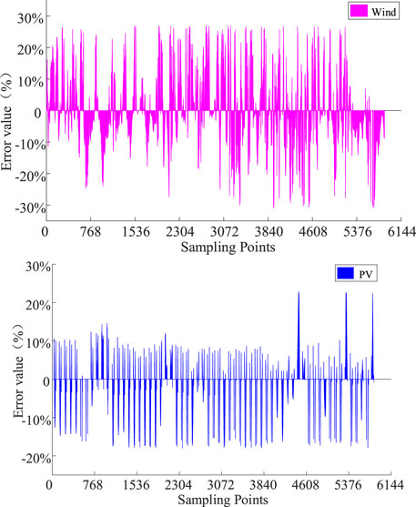
FIGURE 1. Forecast error values for wind and PV.

2.2 Error Randomness Simulation

In this paper, the nonparametric kernel density estimation method is used to obtain the probability distribution of the respective predictions based on the statistical historical data of the scenarios. Compared with the parametric method, the error distribution function does not have to be assumed in advance, which reduces the influence of uncertain factors on the probability model (Li et al., 2019). If $p_r=\left\{p_{r1},p_{r2},\cdots ,p_{rn}\right\}$ is the sample space of the renewable energy forecast error data, $n$ is the sample size. Then the probability density function of the renewable energy forecast error can be expressed as

$f\left(p_r\right)=\frac{1}{nh}{\displaystyle \sum _{i=1}^{n}K\left(\frac{p_r-p_{ri}}{h}\right)}=\frac{1}{n}{\displaystyle \sum _{i=1}^{n}K\left(p_r-p_{ri}\right)}(2)$

$K\left(p\right)=\frac{1}{\sqrt{2\pi }}\exp \left(-\frac{1}{2}{p}^2\right)(3)$

Where $p_{ri}$ is the forecast error sample $i$ of wind power or PV output. $h$ is the bandwidth. $K\left(p\right)$ is the Gaussian kernel function.

A high or low bandwidth $h$ will directly affect the probability density distribution of the prediction error. In order to minimize the prediction error, the optimal bandwidth model is described in Lang et al. (2020). The Gaussian kernel function is settled and the normal distribution $N\left(\mu ,\sigma \right)$ is used as the reference distribution of the probability density function $f\left(p_r\right)$. The optimal bandwidth can be obtained as

$h_{AMISE}=1.06\sigma n^{-1/5}(4)$

Where $\sigma$ is the sample standard deviation.

After using the above method to determine the probability distribution function of wind power output forecast error, and based on the idea of stratified sampling, latin hypercube sampling is used to generate the initial scenarios of large-scale error. In order to effectively simulate the error uncertainty and ensure the model calculation efficiency. The synchronous back-substitution reduction method is used to remove a large number of similar scenarios, retain some representative scenarios, and obtain the corresponding probability of each scenario through calculation. As a result, the uncertain problem is transformed into a deterministic problem. The detailed steps are as follows:

1) Suppose $x_1,x_2,\cdots ,x_T$ are $T$ independent random variables, and their cumulative probability distribution function (wind or PV) is as follows

${\mathrm{\Phi }}_t=F_h\left(x_t\right),{\mathrm{\Phi }}_t\in \left[\mathrm{0,1}\right],t=\mathrm{1,2},\cdots ,T(5)$

2) Assuming that $M$ represents the sampling scale, the ordinate of the cumulative probability distribution function curve ${\mathrm{\Phi }}_t=F_h\left(x_t\right)$ is divided into $M$ equal intervals with a width of 1/M, then the width of each interval is $\left[\left(n-1\right)/M,n/M\right]$, where $\left(n=\mathrm{1,2},\mathrm{...},M\right)$.

3) Select the sampling value of ${\mathrm{\Phi }}_t$ at the midpoint of each interval, and calculate the sampling value of $x_t$ by inverting the cumulative distribution function ${\mathrm{\Phi }}_t=F_h\left(x_t\right)$, that is, the $m^{th}$ sampling value of $x_t$ is as follows

$x_{tm}=F_h^{-1}\left(\frac{m-0.5}{M}\right),t=\mathrm{1,2},\cdots ,T(6)$

4) All the sampled values $x_{tm}$ can form a $T\times M$ initial sampling matrix X. For large-scale scenarios $X=\left\{X_1,X_2,\mathrm{...},X_M\right\}$, set the number of scenarios to be deleted as K.

5) Calculate the Kantorovich distance for each pair scenarios:

$KD\left(X_i,X_j\right)=\sqrt{{\displaystyle \sum _{t=1}^T{\left(x_{t,i}-x_{t,j}\right)}^2}}(7)$

6) For each scenario $X_i$, the distance between each pair of scenarios is calculated separately to find the scenario with the smallest distance from scenario $X_i$. The deletion is performed according to the principle of scenario reduction, and the probability values corresponding to the deleted scenarios are summed up as the probability of occurrence of scenario $X_i$.

7) Repeat step 6 until the number of deleted scenarios reaches K. Finally, the reduced wind power and PV output scenarios and the corresponding scenario probabilities can be obtained.

3 Intraday Rolling Scheduling Model Based on Two-Stage Stochastic Planning

3.1 Two-Stage Stochastic Programming Theory

Consider the existence of random variables and the inconsistent response speed of decision variables. The slow-response decision variable (starting and stopping of the unit) needs to be determined before random variables start to appear. Decision variables with faster response speed (unit ramping, etc.) are not limited, and can be determined after more accurate random variables (such as the regularly updated ultra-short-term forecast output of renewable energy sources). Therefore, this paper introduces a two-stage stochastic programming model (George, 1955), the form is as follows

$\{\begin{array}{l}{\min }_z.c^{T}z+E_s\left\{Q\left(z,s\right)\right\}\\ s.t.Az\le b\\ z\ge 0\end{array}Q\left(x,s\right)=\{\begin{array}{l}{\min }_{y_s}{q}_s^T{y}_s\hfill \\ s.t.W_s{y}_s\le h_s-T_{s}z\hfill \\ y_s\ge 0,\forall s\in \mathrm{\Omega }\hfill \end{array}(8)$

Where $z$ and $y_s$ are the decision variables of the first and second stages. The variables in both stages are greater than zero. $c^{\text{T}}$, $q_s^{\text{T}}$, $b$, $h_s$, $A$, $T_s$ and $W_s$ are known vectors and coefficient matrices. $E_s$ is the expected value under scenario $s$ in the second-stage planning, which can be used to evaluate the volatility of the random variable in the objective function $c^{T}z+Q\left(z,s\right)$. $\Omega$ is the set of all possible scenarios. Since the equation contains random variables, it cannot be solved directly. Random variables can be replaced by calculating expected values. Convert uncertain problems to deterministic ones.

3.2 Intraday Optimization Scheduling Model

This paper establishes a source-load-storage rolling schedule based on a two-stage stochastic programming algorithm. The first stage is to determine the start-stop combination of the following units. Based on the determined start-stop decision of the unit, after the random variable arrives, the output of the unit is adjusted in the second stage to meet the changing demand of the renewable energy output. Intraday dispatch mainly utilizes the feature that the forecast accuracy of renewable energy is negatively correlated with forecast horizon. Combined with regularly updated ultra-short-term forecast data of wind, PV and load, periodic adjustment and revision of the system’s day-ahead plan aims to achieve the effect of global optimization of the system’s output plan. The intraday scheduling of this paper takes 15 min as an interval and 4 h as a cycle. The system automatically updates and obtains ultra-short-term forecast information of wind, PV and load for the next 4 h every 15 min. The rolling timing is shown in Figure 2.

FIGURE 2

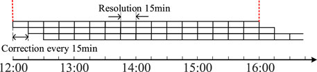
FIGURE 2. Intraday scheduling sequence diagram.

3.2.1 Objective Function

By considering the wind and solar power characteristics, in the first stage the goal is to minimize the start and stop costs of the following units. In the second stage, the goal is to minimize the expected value of the sum of the system operating cost and the correction cost of the initial and final storage capacity of the pumped-storage reservoir, it can be expressed as

$\min C^{on\_off}+E\left(C^{roll}+C^M\right)(9)$

1) Start and stop costs in the first phase

$C^{on\_off}={\displaystyle \sum _{t=1}^T{\displaystyle \sum _{j=1}^{N_q}\left(1-I_{j,t-1}\right)}}{I}_{j,t}{\chi }_{q,j}+{\displaystyle \sum _{t=1}^T{\displaystyle \sum _{i=1}^{N_p}\left[{\chi }_p{I}_{i,t}^p\left(1-I_{i,t-1}^p\right)+{\chi }_g{I}_{i,t}^g\left(1-I_{i,t-1}^g\right)\right]}}(10)$

Where $T$ is the number of scheduling periods. $N_q$ is the number of gas turbine units. ${\chi }_{q,j}$ is the start-up cost of gas turbine $j$. $I_{j,t}$ is the operating state variable of the gas turbine unit $j$ in the time period $t$. $N_p$ is the number of pumped storage units. ${\chi }_p$ and ${\chi }_g$ are the start-up cost coefficients of pumping and power generation for pumped storage units. $I_{i,t}^p$ and $I_{i,t}^g$ are the state variables of pumping and power generation of pumped storage unit $i$ in time period $t$.

2) Expected cost of operating the system in the second stage

$C^{roll}={\displaystyle \sum _{s=1}^{N_S}\omega \left(s\right)\left\{{\displaystyle \sum _{t=1}^T{\displaystyle \sum _{j=1}^{N_q}\left({\alpha }_{q,j}{\left(P_{q,s,j,t}^{roll}\right)}^2+{\beta }_{q,j}{P}_{q,s,j,t}^{roll}+{\gamma }_{q,j}\right)}}+{\displaystyle \sum _{t=1}^T{\displaystyle \sum _{i=1}^{N_{th}}\left({\alpha }_{th,i}{\left(P_{th,s,i,t}^{roll}\right)}^2+{\beta }_{th,i}{P}_{th,s,i,t}^{roll}+{\gamma }_{th,i}\right)}}\right\}}(11)$

Where $\omega \left(s\right)$ is the probability of scenario $s$. ${\text{N}}_{\text{s}}$ is the total number of scenarios. ${\text{N}}_{\text{th}}$ is the number of thermal power units. ${\alpha }_{th,i}$, ${\beta }_{th,i}$ and ${\gamma }_{th,i}$ are the operating cost coefficients of thermal power unit $i$. $P_{th,s,i,t}^{roll}$ is the intraday active power output of thermal power unit $i$ in time period $t$ under scenario $s$. ${\alpha }_{q,j}$, ${\beta }_{q,j}$ and ${\gamma }_{q,j}$ are operating cost coefficients of gas turbine unit $j$. $P_{q,s,j,t}^{roll}$ is the output of gas turbine $j$ in time period $t$ under scenario $s$.

3) Correction costs for the initial and final capacity of the reservoir in the second stage

In the objective function of the second stage of the model, the correction cost of the inconsistency of the reservoir capacity between the beginning and the end of the pumped storage power station is added. Compared with only considering the operating cost of the pumped storage unit, the phenomenon of only pumping or generating electricity during the optimization period is effectively avoided. Its form is as follows

$C^M={\displaystyle \sum _{s=1}^{N_S}\omega \left(s\right)}\mu \left(E_{p,s,T}-E_{p,0}\right)(12)$

Where $\mu$ is the cost correction factor of pumped storage. $E_{p,0}$ and $E_{p,s,T}$ are the initial and terminal capacities of the reservoir.

3.2.2 Constraints in the First Stage

The main decision in the first stage follows the start-stop status of the unit. Relevant minimum on-off time constraints must be met.

1) Start-Stop constraints for gas turbines

$\left(I_{j,t-1}-I_{j,t}\right)\left(T_{\mathit{o}ff,j,t-1}-T_{off.j}\right)\ge 0(13)$

$\left(I_{j,t}-I_{j,t-1}\right)\left(T_{on,j.t-1}-T_{on,j}\right)\ge 0(14)$

where $T_{on,j}$ and $T_{off.j}$ are the minimum running and shutdown times of gas turbine $j$. $T_{on,j.t-1}$ and $T_{off,j,t-1}$ are the running time and shutdown time of gas turbine $j$ to period $t-1$.

2) Constraints between pumped-storage power plants and units

In order to avoid the pumping state of each unit of the pumped storage power station at the same time. Constraints on the states of pumped-storage units and power stations are required. Its form is as follows

$0\le I_{i,t}^p+I_{i,t}^g\le 1(15)$

${\displaystyle \sum _{i=1}^{N_p}{I}_{i,t}^p}\ast {\displaystyle \sum _{i=1}^{N_p}{I}_{i,t}^g}=0(16)$

3) Start and stop constraints of pumped storage units

$\left(I_{i,t-1}^p-I_{i,t}^p\right)\left(T_{on,i.t-1}^p-T_{on,i}^p\right)\ge 0(17)$

$\left(I_{i,t}^p-I_{i,t-1}^p\right)\left(T_{off,i.t-1}^p-T_{off,i}^p\right)\ge 0(18)$

Where $T_{on,j}^p$ and $T_{off,j}^p$ are the minimum operation and shutdown time of the pumped storage unit $i$. $T_{on,j.t-1}$ and $T_{off,j,t-1}$ are the operation and shutdown time of pumped storage unit $i$ to period $t-1$.

4) Constraints on start-stop times of pumped-storage units

The number of state transitions of pumped storage units is limited from the perspective of technology and economy (Xu et al., 2013). Its form is as follows

${\displaystyle \sum _{t=2}^T{I}_{i,t}^g\left(1-I_{i,t-1}^g\right)}\le {\psi }_{g,i}(19)$

${\displaystyle \sum _{t=2}^T{I}_{i,t}^p\left(1-I_{i,t-1}^p\right)}\le {\psi }_{p,i}(20)$

Where ${\psi }_{g,i}$ and ${\psi }_{p,i}$ are the maximum start times of power generation and pumping of pumped storage unit $i$.

3.2.3 Constraints in the Second Stage

The first stage determines only some of the decision variables. The decision variable of the second stage is the daily output of the unit in each scenario, which needs to meet the following general operation constraints.

1) System power balancing constraints

${\displaystyle \sum _{i=1}^{N_{th}}\left(P_{th,s,i,t}^{roll}-P_{th,i,t}^{da}\right)}+{\displaystyle \sum _{j=1}^{N_q}{P}_{q,s,j,t}^{roll}}+{\displaystyle \sum _{i=1}^{N_p}{P}_{g,s,i,t}^{roll}}={\displaystyle \sum _{i=1}^{N_p}{P}_{p,s,i,t}^{roll}}+\mathrm{\Delta }{P}_{ld,t}-\mathrm{\Delta }{P}_{w,s,t}-\Delta P_{pv,s,t}(21)$

Where $P_{th,i,t}^{da}$ is the daily planned output of thermal power unit $i$ in time period $t$ under scenario $s$. $P_{g,s,i,t}^{roll}$ and $P_{p,s,i,t}^{roll}$ are the power generation and pumping power of pumped storage unit $i$ in time period $t$ under scenario s. $\mathrm{\Delta }{P}_{\text{ld,}t}$, $\mathrm{\Delta }{P}_{s,t}^w$ and $\mathrm{\Delta }{P}_{s,t}^{pv}$ are the ultra-short-term and short-term predicted output deviations of load, wind and PV. Its form is as follows

$\mathrm{\Delta }{P}_{w,s,t}=P_{w,s,t}^{roll}-P_{w,t}^{da},\mathrm{\Delta }{P}_{pv,s,t}=P_{pv,s,t}^{roll}-P_{pv,t}^{da},\mathrm{\Delta }{P}_{ld,t}=P_{ld,t}^{roll}-P_{ld,t}^{da}(22)$

Where $P_{w,s,t}^{roll}$, $P_{pv,s,t}^{roll}$ and $P_{ld\text{,}t}^{roll}$ are the ultra-short-term forecasts of wind, PV and load. $P_{w,t}^{da}$, $P_{pv,t}^{da}$ and $P_{ld\text{,}t}^{da}$ are the short-term forecasts of wind, PV and load.

2) Gas turbine constraints

$I_{j,t}{P}_{q,j,\min }\le P_{q,s,j,t}^{roll}\le I_{j,t}{P}_{q,j,\max }(23)$

$-P_{q,j,down}\le P_{q,s,j,t}^{roll}-P_{q,s.j.t-1}^{roll}\le P_{q,j.up}(24)$

Where $P_{q,j,\max }$ and $P_{q,j,\min }$ are the maximum and minimum outputs of the gas turbine j. $P_{q,j.up}$ and $P_{q,j,down}$ are the ramp rate limits for gas turbine $j$.

3) Pumping and generating power constraints

$0\le P_{g,s,i,t}^{roll}\le I_{i,t}^g{P}_{g,i}^{\max }(25)$

$0\le P_{p,s,i,t}^{roll}\le I_{i,t}^p{P}_{p,i}^{\max }(26)$

Where $P_{g,i}^{\max }$ and $P_{p,i}^{\max }$ are the maximum power generation and pumping power of the pumped storage unit $i$.

4) Upper reservoir capacity constraints

$E_{p,\min }\le E_{p,s,t}\le E_{p,\max }(27)$

$E_{p,s,t}=E_{p,s,t-1}+{\displaystyle \sum _{i=1}^{N_P}\left(I_{i,t}^p{P}_{p,s,i,t}^{roll}-I_{i,t}^g{P}_{g,s,i,t}^{roll}/{\eta }_{dis}\right)}\mathrm{\Delta }t(28)$

Where $E_{\max }$ and $E_{\min }$ are the limits of the reservoir capacity. $E_{p,s,t}$ is the capacity of the reservoir in the scenario $s$ in the time period $t$. ${\eta }_{\text{dis}}$ is the energy conversion efficiency of the pumped storage unit.

5) Reservoir starting and ending storage capacity constraints

In order to avoid the phenomenon that the pumped storage power station releases water to reduce the storage capacity to absorb the abandoned wind during the optimization period, this paper relaxes the capacity of the end of the reservoir based on the initial storage capacity (Hu et al., 2012). It can be expressed as

$\mathrm{\Delta }{E}_{\min }\le E_{p,0}-E_{p,s,T}\le \mathrm{\Delta }{E}_{\max }(29)$

Where $\mathrm{\Delta }{E}_{\max }$ and $\mathrm{\Delta }{E}_{\min }$ are the upper and lower limits of the reservoir capacity deviation during the beginning and end periods.

6) Line active power flow constraint

$P_{th,s,t,l}^{roll}+P_{q,s,t,l}^{roll}+P_{s,t,l}^w+P_{s,t,l}^{pv}+P_{g,s,t,l}^{roll}-P_{p,s,t,l}^{roll}-P_{ld,t.l}={\displaystyle \sum _l\left({\delta }_{t,l}-{\delta }_{t,k}\right)/X_{l-k}}(30)$

$P_{l-k,\min }\le {\displaystyle \sum _l\left({\delta }_{t,l}-{\delta }_{t,k}\right)/X_{l-k}\le P_{l-k,\max }}(31)$

Where $P_{th,s,t,l}^{roll}$, $P_{q,s,t,l}^{roll}$, $P_{s,t,l}^w$, $P_{s,t,l}^{pv}$, $P_{p,s,t,l}^{roll}$, $P_{g,s,t,l}^{roll}$, and $P_{ld,t.l}$ are the powers of thermal power units, gas turbines, wind farms, PV power plants, pumped storage, power generation and loads at node $l$ in scenario $s$. ${\delta }_{t,l}$ and ${\delta }_{t,k}$ are the phase angles of nodes $l$ and $k$ at time period $t$. $X_{l-k}$ is the reactance value of branch $l-k$. $P_{l-k,\max }$ and $P_{l-k,\min }$ are the upper and lower limits of the active power allowed to be delivered in the branch $l-k$.

7) Rolling plan revision constraints

$P_{th,s,i,t}^{roll}-P_{th,i,t}^{da}\ge \max \left(P_{th,i,t}^{\min }-P_{th,s,i,t}^{roll},P_{th,i,t}^{da}+\mathrm{\Delta }{\overline{p}}_{th,i}-P_{th,s,i,t}^{roll}\right)(32)$

$P_{th,s,i,t}^{roll}-P_{th,i,t}^{da}\le \min \left(P_{th,i,t}^{\max }-P_{th,s,i,t}^{roll},P_{th,i,t}^{da}+\mathrm{\Delta }{\overline{p}}_{th,i}-P_{th,s,i,t}^{roll}\right)(33)$

Where $\mathrm{\Delta }{\overline{p}}_{th,i}$ is the maximum value of the difference between the intraday output plan and the day-ahead planned output of thermal power unit $i$.

8) Unit output constraints

$0\le P_{w,s,t}^{roll}\le P_{w,}^{pre},0\le P_{pv,s,t}^{roll}\le P_{pv,\max }^{pre},P_{th,i}^{\min }\le P_{th,s,i,t}^{roll}\le P_{th,i}^{\max }(34)$

where $P_w^{\text{pre}}$ and $P_{pv,\max }^{\text{pre}}$ are the predicted output values of wind power and PV; $P_{th,i}^{\max }$ and $P_{th,i}^{\min }$ are the upper and lower output limits of thermal power unit $i$.

9) Thermal power unit ramping constraint

$-P_{th,i,down}\le P_{th,s,i,t}^{roll}-P_{th,s.i.t-1}^{roll}\le P_{th,i.up}(35)$

where $P_{th,i.up}$ and $P_{th,i,down}$ are the upper and lower ramping limits of thermal power unit $i$.

Eqs 9–35 are the intraday rolling scheduling model based on two-stage stochastic planning. The fundamental difference between this model and the traditional intraday optimal scheduling model of stochastic programming is that in the first-stage decision-making process, the operating state of the following unit is first determined. Considering that the start-stop response of the unit is slow, but the climbing speed of the following unit is faster. Therefore, in the second stage planning, the output of each unit is optimized by the decision of the first stage. During the whole decision-making process, the start-stop combination of thermal power units remains unchanged as planned.

3.3 Solve the Model

Considering the operating cost of thermal power units in the objective function as a nonlinear quadratic function, the quadratic function in the objective function can be linearized by its linearization through segment linearization (Carrion and Arroyo, 2006). The core idea of the linearization process is to divide the quadratic function into $m$ segmented functions. Then, the slope of each segmented function is found and converted into a primary function with respect to the horizontal coordinate, and thus the linearization of the quadratic function is realized. The linearization principle diagram of thermal power unit operating cost segments is shown in Figure 3. The operating interval of thermal power unit $i$ is divided into $m$ ($m=3$) segments, and the value of $m$ should be chosen appropriately. the smaller $m$ is, the less linearization accuracy will be achieved. the larger $m$ is, the higher linearization accuracy will be achieved, and at the same time, it will increase the size of the decision variables, which makes it difficult to solve the calculation later. $Z_{th,i}^0$ denotes the operating cost of thermal power unit $i$ at the lowest level of output. $Z_{th,i}^{seg}$ is the segmentation point of segment $seg$ ($seg=\left\{\mathrm{1,2,3}\right\}$). $\Delta P_{th,i}^{seg}$ is the length of each segment. length of each segment interval. $K_{th,i}^{seg}$ is the slope of segment $seg$. $Z_{th,i}^{seg}$, $\Delta P_{th,i}^{seg}$ and $K_{th,i}^{seg}$ should satisfy the following constraints

$\{\begin{array}{l}\mathrm{\Delta }{P}_{th,i}^{seg}=\frac{P_{th,i}^{\max }-P_{th,i}^{\min }}{m}\hfill \\ K_{th,i}^{seg}=\frac{C_{th,i,t}\left(Z_{th,i}^{seg}\right)-C_{th,i,t}\left(Z_{th,i}^{seg-1}\right)}{Z_{th,i}^{seg}-Z_{th,i}^{s-1}}\hfill \\ Z_{th,i}^{seg}=Z_{th,i}^0+seg\cdot \mathrm{\Delta }{P}_{th,i}^{seg}\hfill \\ Z_{th,i}^0=P_{th,i}^{\min }\hfill \end{array}(36)$

FIGURE 3

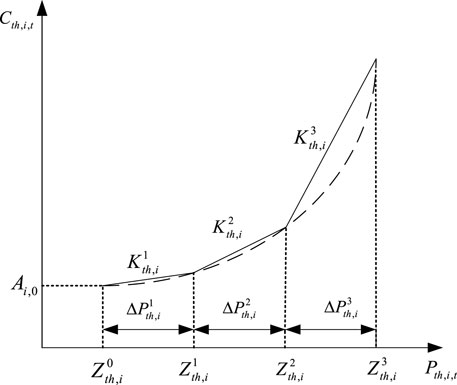
FIGURE 3. Segmented linearization of operating costs of thermal power units.

After linearization, the operating cost of thermal power unit $i$ is converted to the following model:

$\{\begin{array}{l}{C}_{th,i,t}\left(P_{th,i,t}\right)=A_{i,0}+{\displaystyle \sum _m^{seg=1}\left(K_{th,i}^{seg}\cdot \mathrm{\Delta }{P}_{th,i}^{seg}\right)}\\ P_{th,i,t}=P_{th,i}^{\min }+{\displaystyle \sum _m^{seg=1}\left(\mathrm{\Delta }{P}_{th,i}^{seg}\right)}\\ 0\le \mathrm{\Delta }{P}_{th,i}^{seg}\le Z_{th,i}^{seg}-Z_{th,i}^{seg-1}\\ A_{i,0}={\alpha }_{th,i}{\left(P_{th,i,t}\right)}^2+{\beta }_{th,i}{P}_{th,i,t}+{\gamma }_{th,i}\end{array}(37)$

Referring to the linearization process of thermal power units, the operating cost of gas turbines can be linearized similarly.

The start-up cost of pumped storage in the objective function is a bilinear nonlinear programming problem that can be linearized using McCormick’s inequality (Castro and Pedro, 2015). Taking the pumped start-up cost $I_{i,t}^{\text{p}}{I}_{i,t-1}^{\text{p}}$ as an example, by introducing a new binary integer variable $I_{i,t}^{\text{y}}$ and making $I_{i,t}^{\text{y}}=I_{i,t}^{\text{p}}{I}_{i,t-1}^{\text{p}}$, the equation can be equated to the following linear constraint

$\{\begin{array}{l}0\le I_{i,t}^y\le I_{i,t}^p\\ I_{i,t}^y\le I_{i,t-1}^p\\ I_{i,t}^p+I_{i,t-1}^p-1\le I_{i,t}^y\end{array},I_{i,t}^y=I_{i,t}^p{I}_{i,t-1}^p(38)$

Referring to the processing method of $I_{i,t}^{\text{p}}{I}_{i,t-1}^{\text{p}}$, ${\text{I}}_{i,t}^{\text{g}}{I}_{i,t-1}^{\text{g}}$ and $I_{j,t}{I}_{j,t-1}$ can be similarly linearized.

After the linearization process, the model built in this paper belongs to the mixed integer linear programming problem. By writing a program in the YALMIP environment of MATLAB and calling the solver GUROBI to solve the model, the optimal output combination of each unit is obtained.

4 Case Study

4.1 Basic Data

In the case study, the power system in this paper includes five thermal power units, two gas turbines, a pumped-storage power station, a wind farm and a PV power station. The installed capacity of wind farm and PV power station in the system is 400 and 250 MW respectively. There are five thermal power units and two gas turbines, and the specific parameters are shown in Table 1. A pumped storage power plant with an installed capacity of 60 MW, the upper reservoir storage limit and the initial reservoir capacity of this pumped storage power plant are 600 MWh and 300 MWh. Figure 4 shows the rolling updated ultra-short-term power forecasting curves for wind, PV and load. Figure 5 gives the day-ahead operation plan curves for thermal units, where the day-ahead plan identifies three thermal units to be put into operation.

TABLE 1

TABLE 1. Basic data of conventional thermal power units and gas turbines.

FIGURE 4

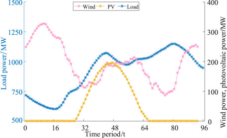
FIGURE 4. Ultra-short-term forecast curves for wind, PV and load.

FIGURE 5

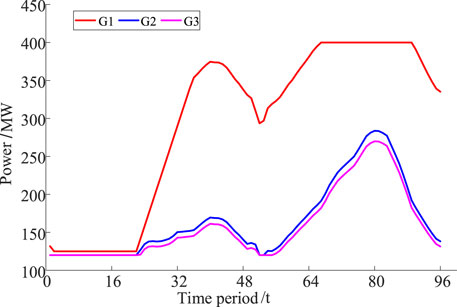
FIGURE 5. Day-ahead planned output curves of thermal power units.

Figure 6 shows three representative sequences of wind power errors obtained after generating 200 initial scenarios using the method described in Section 2, with probabilities of 0.46, 0.305 and 0.235, respectively. The PV error curve can also be obtained this manner. The following three scenarios are set to verify the effectiveness of the proposed dispatching model for making dispatching plans in high-penetration renewable energy power systems.

Case 1: Day-ahead scheduling without the participation of quick start and stop groups.

Case 2: Intraday scheduling of following units such as pumped storage and gas turbines is considered. However, the start-stop combination of fast units is not considered in the intraday schedule.

Case 3: Intraday scheduling of following units such as pumped storage and gas turbines is considered. The two-stage stochastic planning model established in this paper is used. In the first stage, the start-stop status of the following units is determined. In the second stage, the intraday deviations are coordinated to find the optimal unit output.

FIGURE 6

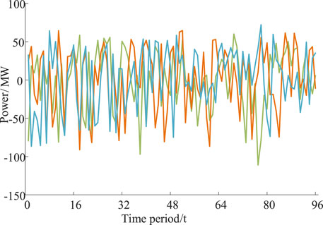
FIGURE 6. Wind power error representation scenarios.

4.2 Analysis of the Output of the Units

The intraday output curves of thermal units and gas turbines for case 2 and 3 are shown in Figures 7, 8. Since case 2 does not consider the start-stop combination of fast units during the day, the gas turbines are on during the optimized hours. The downward adjustment space of the system in the night abandonment interval is reduced, which leads to the limitation of wind power feed-in power. The gas turbines in case 3 need to be called up only during the nighttime peak of the load (19:30-20:15) according to the regulation demand. This reduces the operating cost of the gas turbine and provides more adjustable space for the system in case 3 during the optimization period. The output curve of the thermal unit shows that the thermal unit in case 3 has a smoother climb.

FIGURE 7

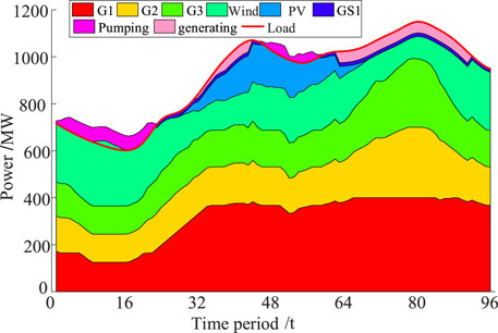
FIGURE 7. Unit output curves of Case 2.

FIGURE 8

FIGURE 8. Unit output curves of Case 3.

Figures 9, 10 show the change curves of pumped storage unit output and reservoir capacity under case 2 and case 3. The model built in this paper relaxes the capacity of the end of the reservoir and considers the correction cost of inconsistency between the beginning and end of the reservoir. It can effectively avoid the phenomenon that the pumped-storage unit has been pumping water and generating electricity when the program is running, and the effect of the unit call is not obvious. As can be seen from the figure below, pumped storage is mainly used to store energy during the nighttime wind power generation, and is used as the power generation side to provide increased capacity for the system during the peak load period. The analysis shows that the number of power generation starts of the pumped storage unit in the two cases remains the same. However, the number of pumping starts in case 3 is reduced by two on the basis of case 2, which increases the flexibility, safety and economy of the system.

FIGURE 9

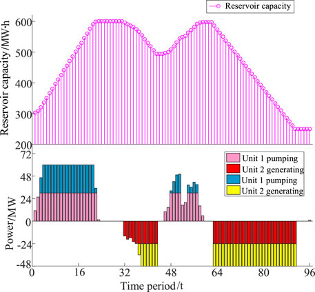
FIGURE 9. Reservoir capacity and unit output curve of Case 2.

FIGURE 10

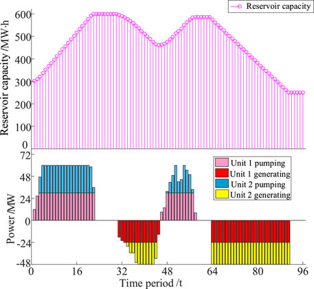
FIGURE 10. Reservoir capacity and unit output curve of Case 3.

Figure 11 represents the wind power abandoned by the system for each case. Among them, case 1 has a larger amount of wind abandonment. cases 2 and 3 consider fast start-up and shutdown of units during the day, and their abandoned wind power intervals are shortened from the period of 0:15-5:30 at night to 2:15-4:00 and 2:30-3:15, respectively. the total amount of abandoned wind power is reduced from 565.478 MW-h to 25.9581 MWh and 9.1021 MW. Although the abandoned power in case 2 is significantly reduced, the wind power in case 3 is almost fully online. It is able to further increase the dispatchability of renewable energy and the acceptance rate into the grid.

FIGURE 11

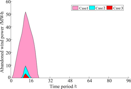
FIGURE 11. Abandoned wind power.

4.3 Economic Analysis

Table 2 shows the total intraday operating costs of the system under each case. Among them, the set system power abandonment penalty fee is 50 yuan/MW. The operating cost of pumped storage includes the start-up and shutdown of pumped storage and the cost of storage capacity correction. Compared with case 1, although case 2 increases the flexibility of unit participation in regulation, the cost of wind curtailment is reduced by 107,903.972 yuan. However, without taking into account the start-stop combination of rapid units under the daily scale, the thermal power operating cost has increased by 51,091.975 yuan on the basis of the previous plan. After considering the running cost of the fast unit, the total cost of the system has increased by 52,984.09 yuan on the basis of the day-ahead plan. In case 3, a two-stage stochastic programming model is adopted and the decision of starting and stopping of rapid units is considered, and the cost of wind curtailment of the system is further reduced by 4,277.0007 yuan. At the same time, the gas turbine and pumped storage unit are called on demand, and the final total system operating cost is reduced by 67,115.3984 yuan on the basis of the previous plan. This shows that the economics of the method in this paper and the absorption effect of wind power are better.

TABLE 2

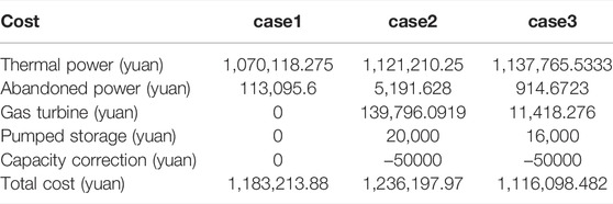
TABLE 2. Scheduling costs of the system in each case.

4.4 Compared With the Optimization Results of Related Literatures

Table 3 compares the cost optimization rate of the intraday scheduling method proposed in this paper with other intraday scheduling methods. Compared with the researches (Cui, et al., 2021.; Jin, et al., 2020) that configures fast units to participate in regulation but does not consider the start-stop combination of fast units, the intraday cost optimization rate is increased by 4.9775 and 2.1219%, respectively. Compared with the research (Ran et al., 2016) based on the rolling scheduling strategy of short-term unit combination, this paper combines the two-stage stochastic programming theory and considers the fast unit participation in the intraday cost optimization rate, which can improve the cost optimization rate by 4.9838%.

TABLE 3

TABLE 3. Comparison with the results of the operating cost of similar literature strategies.

5 Conclusion

1) The rapid start-up and shutdown unit (gas turbine, pumped storage) is used as the following unit dispatched during the day. It can increase the system regulation ability and improve the system’s ability to accept fluctuations in intermittent energy, but at the same time, it will also lead to an increase of 4.3181% in the total operating cost.

2) Based on the two-stage stochastic programming theory, compared with the traditional intraday scheduling that does not take into account the rapid start and stop of units. The model proposed in this paper can reduce the number of start and stop of fast units and avoid unnecessary unit operations. On the basis of the previous plan, the on-grid rate of wind power has increased to 99.806%, and the system economy has increased by 5.6723%.

Data Availability Statement

The raw data supporting the conclusion of this article will be made available by the authors, without undue reservation.

Author Contributions

All of the authors have contributed to this research. Conceptualization, YZ and QJ; method-ology, YZ; software, YZ and QJ; validation, QJ; formal analysis, QJ; investigation, TZ; re-sources, YZ; data curation, YX; writing—original draft preparation, QJ; writing—review and editing, YZ and QJ; visualization, QJ; supervision, YX; project administration, YZ; funding acquisition, YZ.

Funding

This research was supported by the China Key R&D Program Funding Project 2019YFB1505400.

Conflict of Interest

The authors declare that the research was conducted in the absence of any commercial or financial relationships that could be construed as a potential conflict of interest.

Publisher’s Note

All claims expressed in this article are solely those of the authors and do not necessarily represent those of their affiliated organizations, or those of the publisher, the editors and the reviewers. Any product that may be evaluated in this article, or claim that may be made by its manufacturer, is not guaranteed or endorsed by the publisher.

Acknowledgments

Thanks for my dear Senior, Shengkai Guo, Pengxiang Huang, and Pinchao Zhao, for giving my valuable suggestions.

References

Bao, Y., Wang, B., Yang, L., and Yang, S. (2016). A Rolling Dispatch Model Considering Large-Scale Wind Power Connection and Multi-Time Scale Demand Response Resource Coordination Optimization [J]. Chin. J. Electr. Eng. 36 (17), 4589–4600. doi:10.13334/j.0258-8013.pcsee.151343

CrossRef Full Text | Google Scholar

Barth, R., Brand, H., Meibom, P., and Weber, C. (2006). A Stochastic Unit-Commitment Model for the Evaluation of the Impacts of Integration of Large Amounts of Intermittent Wind Power. Int. Conf. Probabilistic Methods Power Syst. (6), 11–15. doi:10.1109/PMAPS.2006.360195

CrossRef Full Text | Google Scholar

Botterud, A., Zhou, Z., Wang, J., Sumaili, J., Keko, H., Mendes, J., et al. (2013). Demand Dispatch and Probabilistic Wind Power Forecasting in Unit Commitment and Economic Dispatch: A Case Study of Illinois. IEEE Trans. Sustain. Energ. 4 (1), 250–261. doi:10.1109/tste.2012.2215631

CrossRef Full Text | Google Scholar

Carrion, M., and Arroyo, J. M. (2006). A Computationally Efficient Mixed-Integer Linear Formulation for the thermal Unit Commitment Problem[J]. IEEE Trans. Power Syst. 21 (3), 1371–1378. doi:10.1109/TPWRS.2006.876672

CrossRef Full Text | Google Scholar

Castro, P. M., and Pedro, M. (2015). Tightening Piecewise McCormick Relaxations for Bilinear Problems. Comput. Chem. Eng. 72, 300–311. doi:10.1016/j.compchemeng.2014.03.025

CrossRef Full Text | Google Scholar

Cui, Y., Zhou, H., Zhong, W., Hui, X., and Zhao, Y. (2021). Day-ahead-day Two-Stage Rolling Optimization Scheduling Considering Generalized Energy Storage and thermal Power Combined Peak Shaving [J]. Power Grid Techn. 45 (01), 10–20. doi:10.13335/j.1000-3673.pst.2020.0206

CrossRef Full Text | Google Scholar

George, B. D. (1955). Linear Programming under Uncertainty[M]. Santa Monica, CA: The Rand Corporation.

Google Scholar

Han, X., Li, T., Zhang, D., and Zhou, X. (2021). New Issues and Key Technologies for New Power System Planning under the Dual Carbon Goal [J]. High Voltage Techn. 47 (09), 3036–3046. doi:10.13336/j.1003-6520.hve.20210809

CrossRef Full Text | Google Scholar

Hu, Z., Ding, H., and Kong, T. (2012). Optimal Scheduling Model for Combined Daily Operation of Wind Power and Pumped Storage [J]. Automation Electric Power Syst. 36 (02), 36–41+57.

Google Scholar

Jin, L., Fang, X., Cai, Z., Chen, D., and Li, Y. (2020). Multi-time-scale Source-Storage-Load Coordination Scheduling Strategy for Power Grid Connected to Energy Storage Power Stations Considering Characteristic Distribution [J]. Power Grid Techn. 44 (10), 3641–3650. doi:10.13335/j.1000-3673.pst.2020.0330

CrossRef Full Text | Google Scholar

Lang, W., Ma, X., Zhou, B., Yang, D., Luo, Y., and Liu, L. (2020). Probability Interval Prediction of Wind Power Based on LSTM and Nonparametric Kernel Density Estimation [J]. Smart Power 48 (02), 31–37+103.

Google Scholar

Li, S., Dai, J., Dong, H., Shen, W., and Ma, X. (2019). Optimal Operation of Wind-Solar Pumping-Storage Hybrid Power Generation System Considering Correlation [J]. J. Electric Power Syst. Automation 31 (11), 92–102. doi:10.19635/j.cnki.csu-epsa.000179

CrossRef Full Text | Google Scholar

Lu, Y. (2021). Accurately Grasp the new era Orientation of My Country's Electric Power Development [J]. China Electric Power Industry 974 (09), 16–17.

Google Scholar

Makarov, Y. V., Etingov, P. V., Ma, J., Huang, Z., and Subbarao, K. (2011). Incorporating Uncertainty of Wind Power Generation Forecast into Power System Operation, Dispatch, and Unit Commitment Procedures. IEEE Trans. Sustain. Energ. 2 (4), 433–442. doi:10.1109/tste.2011.2159254

CrossRef Full Text | Google Scholar

Notton, G., Nivet, M.-L., Voyant, C., Paoli, C., Darras, C., Motte, F., et al. (2018). Intermittent and Stochastic Character of Renewable Energy Sources: Consequences, Cost of Intermittence and Benefit of Forecasting. Renew. Sustain. Energ. Rev. 87 (MAY), 96–105. doi:10.1016/j.rser.2018.02.007

CrossRef Full Text | Google Scholar

Qian, Y., Liu, J., and Jiang, W. (2021). Peak Shaving Strategy of Power System Considering Deep Interaction between Source, Grid, Load and Storage under Different Photovoltaic Penetration Rates [J]. Electric Power Construction 42 (09), 74–84. doi:10.12204/j.issn.1000-7229.2021.09.008

CrossRef Full Text | Google Scholar

Ran, L., Li, Y., and Dang, L. (2016). Research on Rolling Optimization Scheduling of Wind Farms Based on Short-Term Unit Combinations [J]. J. North China Electric Power Univ. (Natural Sci. Edition) 43 (05), 49–54.

Google Scholar

Shang, Z. (2021). SDIC Power: Actively Deploy green Carbon Reduction Investment [J]. Energy 153 (10), 22–24.

Google Scholar

Sheng, G., Qian, Y., Luo, L., Song, H., Liu, Y., and Jiang, X. (2021). Key Technologies for Power Equipment Operation and Maintenance for New Power Systems and Their Application Prospects [J]. High Voltage Techn. 47 (09), 3072–3084.

Google Scholar

Tuohy, A., Peter, M., Denny, E., and O’Malley, M. (2009). Unit Commitment for Systems with Significant Wind Penetration[J]. IEEE Trans. Power Syst. 24 (2). doi:10.1109/tpwrs.2009.2016470

CrossRef Full Text | Google Scholar

Wang, Y., Zhan, H., Hu, X., and Wang, B. (2021). Joint Dispatch of Electric Heating System Considering Source and Load Uncertainty [J]. Smart Electric Power 49 (04), 7–13+29. doi:10.3969/j.issn.1673-7598.2021.04.003

CrossRef Full Text | Google Scholar

Xu, F., Lei, C., Jin, H., and Liu, Z. (2013). Joint Optimization Operation Modeling and Application Analysis of Pumped Storage Power Station and Wind Power [J]. Automation Electric Power Syst. 37 (01), 149–154. doi:10.7500/AEPS201209256

CrossRef Full Text | Google Scholar

Yang, H., Hu, W., Min, Y., Luo, W., Wang, Z., and Ge, W. (2014). Considering the Recently Planned Multi-Objective Coordinated Scheduling of Wind-Storage Combined System [J]. Chin. J. Electr. Eng. 34 (28), 4743–4751. doi:10.13334/j.0258-8013.pcsee.2014.28.001

CrossRef Full Text | Google Scholar

Zhang, B., Wu, W., Zheng, T., and Sun, H. (2011). Design of Active Power Dispatching System with Multi-Time Scale Coordination to Accommodate Large-Scale Wind Power [J]. Automation Electric Power Syst. 35 (01), 1–6.

Google Scholar

Zhang, Y., Zhang, F., Zhu, B., Xiang, Z., Tang, L., Ma, X., et al. (2018). Closed-loop Control System of Daily Rolling Power Generation Plan Suitable for New Energy Power Generation Access [J]. Electric Power Automation Equipment 38 (03), 162–168. doi:10.16081/j.issn.1006-6047.2018.03.022

CrossRef Full Text | Google Scholar