A Motion Planning Algorithm for Live Working Manipulator Integrating PSO and Reinforcement Learning Driven by Model and Data

1 Introduction

With the rapid growth of the economy, electricity demand continues to rise, posing higher and higher challenges to the power supply. To meet these challenges, the application of deep reinforcement learning (Zhang et al., 2018), robotics (Menendez et al., 2017), swarm intelligence (SI) algorithms (Ma et al., 2021c), and other artificial intelligence technologies to solve resource scheduling (Ma et al., 2021d), inspection, maintenance, and others has become the smart grid’s development direction.

The live work of overhauling the circuit under the premise of continuous power supply of the power grid can significantly improve the safety of the power supply. However, there are many restrictions on manual live work due to the danger of live work itself and the working environment. Therefore, it is critical to use technology to replace manual live work with robots. The working environment of live working manipulators is always complicated and ever-changing. So, the major challenge is how to determine a suitable path/trajectory in a complex and changeable environment with obstacles so that the manipulator can reach the target point (Siciliano et al., 2009; Lynch and Park 2017).

The motion planning of manipulators can be divided into two categories: joint angle coordinate motion planning and Cartesian coordinate motion planning. The manipulator’s end-effector is the planning reference object in the Cartesian coordinate. However, due to the inverse kinematics of the manipulator, there may be many problems, such as a lot of calculation, ease to reach the singularity, the near-point in the Cartesian coordinate system taking a large rotation joint angle, and large instantaneous speed (Choset et al., 2005; Gasparetto et al., 2015; Lynch and Park 2017). The motion planning in the joint angular coordinate system differs much from human intuitive feelings, but it can successfully avoid problems in the rectangular coordinate system while also planning the manipulator’s joint angular velocity and angular acceleration. So, it can get a whole trajectory of the manipulator’s joint after planning, which is why it is also known as trajectory planning (Gasparetto et al., 2012; Gasparetto et al., 2015; Lynch and Park 2017).

The obstacle avoidance motion planning of the manipulator has always been a research hotspot. The artificial potential field method (Khatib 1985) is an earlier algorithm, which designs the target position as a gravitational field and the obstacle position as a repulsion field, so that the real-time avoidance of the manipulator can be accomplished. However, such algorithms tend to fall into local minima and move slowly near the obstacles. Some search-based algorithms, such as rapidly exploring random trees (RRTs) (Wei and Ren 2018; Cao et al., 2019), find the obstacle avoidance path of the manipulator through searching, but such algorithms generally only consider obstacle avoidance of the manipulator end-effector and find it too difficult to consider global obstacle avoidance. At the same time, such algorithms also need to increase the computational cost of path smoothing.

In recent years, deep learning and deep reinforcement learning have brought remarkable results to many fields, such as computer vision (Krizhevsky et al., 2017; Yang et al., 2021), natural language processing (Devlin et al., 2019), and industrial process optimization (Ma et al., 2021b). Many achievements have been made using deep learning and deep reinforcement learning for manipulators (Yu et al., 2021; Hao et al., 2022). Wu Yunhua applied the deep reinforcement learning algorithm to the trajectory planning of a space dual manipulator (Wu et al., 2020). Kalashnikov proposed a vision-based closed-loop grasping algorithm framework for manipulators (Kalashnikov et al., 2018). Ignasi Clavera proposed a modular and reward-guided reinforcement learning algorithm for manipulator pushing tasks (Clavera et al., 2017). The intelligence and learning ability of the manipulator are substantially improved by these algorithms; however, the training period is excessively long and consumes more resources. For example, QT-opt (Kalashnikov et al., 2018) employed seven robots and ten GPUs and took 4 months to train.

Model-driven algorithms are built on the foundation of developing a mechanism model, and the correctness of the model is directly tied to the algorithm’s performance. Model-driven algorithms’ key priority is to figure out how to optimize model parameters to improve model performance. Swarm algorithms, such as the genetic algorithm (GA) (Holland 1992), particle swarm optimization (PSO) (Kennedy and Eberhart 1995), and brainstorming optimization (BSO) (Shi 2011), are commonly used in parameter optimization. In difficult multi-objective optimization situations, these algorithms can get good results (Ma et al., 2021a; Ma et al., 2021c). In the aspect of manipulator motion planning, some achievements have been made in optimizing the parameters of the trajectory model by using the swarm intelligence algorithm. The trajectory model after optimizing the parameters can make the robotic arm avoid obstacles and successfully reach the target point (Rulong and Wang 2014; Wang et al., 2015). However, such algorithms rely on offline training and find it difficult to avoid obstacles in real time. When the environment changes, the algorithms must be retrained and generalization capacity becomes poor. Furthermore, these methods are incapable of avoiding model-building errors.

Based on the above research, this research provides a hybrid data-model–driven algorithm framework that can avoid non-essential exploration during the early stages of deep reinforcement learning and can solve the problems of model-driven algorithms’ poor generalization. The main contributions are as follows:

1) A framework for algorithms driven by data and model, which uses the reward function to merge model-driven and data-driven algorithms, is proposed.

2) The P-SAC algorithm, which mixed PSO and SAC, is proposed based on the proposed hybrid data-model–driven algorithm framework. The algorithm optimizes the model parameters with PSO first and then pre-trains the agent before letting it study to interact with the environment.

3) P-SAC is applied to the motion planning of the live working manipulator, and the manipulator can successfully reach the target point without colliding with obstacles. Compared with the SAC that is not model-driven, P-SAC has a faster convergence speed and better final performance.

2 Background and Problem Statement

2.1 Motion Planning of Manipulator

The motion planning problem of the manipulator can be described as follows.

Given the source point $P_s\left(P_s\in {\mathrm{ℝ}}^3\right)$, the goal point $P_g\left(P_g\in {\mathrm{ℝ}}^3\right)$, and the obstacle information $Inf{o}_{ob}$, finding a motion path $g\left(t\right)$ allows the manipulator to reach the target point and avoid obstacles during the motion. In general, $P_s$ and $P_g$ are the coordinates in the Cartesian coordinate system of the end of the manipulator. We need to obtain the inverse solution of them to obtain the joint angle coordinates $q_s,q_g\left(q_s,q_g\in {\mathrm{ℝ}}^n,n is the DOF ofmanipulator\right)$ of the manipulator. At the same time, during the movement, the joint angle of the manipulator should not have a sudden change point, that is, the joint angular velocity of the manipulator can be obtained, and the angular velocity should not have a sudden change point. So, the motion planning problem of the manipulator can be described in mathematical language as follows.

Definition 1: Let $g\left(t\right),$ which satisfies the following conditions:

$g\left(0\right)=q_s,$

$g\left(T\right)=q_g,$

$g\left(t\right) not collide with Obstacle with Inf{o}_{ob},0\le t\le T,$

$g\prime \left(t\right) and g″\left(t\right) existed, 0\le t\le T,$

$q_s,q_g,g\prime \left(t\right)\in {\mathrm{ℝ}}^n.$

2.2 PSO

In 1995, Kennedy and Eberhart (1995) proposed a particle swarm optimization algorithm based on the idea of birds foraging. In PSO, the potential solution to the optimization problem is a “particle” in the search space, and all particles have two properties: fitness value and speed. The fitness value is determined by the function to be optimized. And the larger fitness value (or smaller) means the particle is better. The speed determines the flying direction and distance of the particle. The process of PSO is that the particle follows the current optimal particle to search in the solution space.

2.3 SAC

Deep reinforcement learning combines the data representation ability of deep learning and the decision-making ability of reinforcement learning. In 2013, the proposal of the DQN (Mnih et al., 2013) algorithm marked the beginning of the era of deep reinforcement learning algorithms. Since DQN is difficult to solve the continuous action space problem, Lillicrap Timothy proposed DDPG, which combined with the actor–critic framework (Lillicrap et al., 2019). However, the DDPG algorithm is sensitive to hyperparameters and is challenging to use, so the SAC (Haarnoja et al., 2018; Haarnoja et al., 2019) algorithm is proposed.

SAC introduces the entropy of the strategy into the objective function to maximize the expected cumulative return while making the strategy as random as possible. Its objective function is as follows:

${\pi }^{\text{*}}=arg\max {\mathbb{E}}_{\tau \sim \pi }\left[{\displaystyle {\sum }_{t=0}^{\infty }{\gamma }^t}\left(R\left(s_t,a_t\right)+\alpha H\left(\pi \left(\cdot |s_t\right)\right)\right)\right].$

The temperature coefficient $\alpha$ is used to determine the importance of the entropy item to the reward item. The SAC algorithm improves the robustness of the algorithm by adding the entropy of the policy to the objective function.

3 P-SAC: An Algorithm That Fuses PSO and Reinforcement Learning

3.1 A Framework for Algorithms Driven by Data and Model

There are a lot of ineffective explorations in the early stages of deep reinforcement learning, and model-driven algorithms cannot avoid errors in model design and lack intelligence. As illustrated in Figure 1, this research provides a hybrid data-model–driven algorithm framework. The details are as follows:

1) $Env\stackrel{simply}{\Rightarrow }\mathrm{ℳ }\&\mathcal{ C}$. Simplify the model ($\mathrm{ℳ}$) according to the environment and the task to be solved and design a controller ($\mathcal{C}$) if necessary.

2) $\mathrm{ℳ }\&\mathcal{ C}\stackrel{ SI optimize parameters }{\Rightarrow }\mathrm{ ℳ }\&\mathcal{ C}$. Employ the SI algorithm to optimize parameters to create a better controller or model.

3) $\mathrm{ℳ }\&\mathcal{ C}\Rightarrow <S,A>\stackrel{env\mathcal{C}R}{\Rightarrow }{D}_1:<S,A,R,S\_,Done>$. Use the optimized model or controller to obtain the required data $<S,A>$ and then use the reward function ($R$) to convert $<S,A>$ into $D_1<S,A,R,S\_,Done>$.

4) $D_1\stackrel{pretrain }{\Rightarrow }Agent$. Use $D_1$ to pre-train the agent, so that the agent has a certain intelligence.

5) $Agent\iff Env.$ The agent learns from the environment to improve the algorithm’s generalization performance.

FIGURE 1

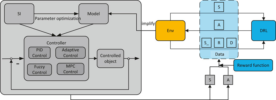
FIGURE 1. Framework for algorithms driven by data and model.

3.2 Model-Driven Part Design

3.2.1 DH Model of the Live Working Manipulator

The motion planning of the manipulator inevitably involves the forward and inverse kinematics of the manipulator, that is, getting the position and pose of the manipulator’s end-effector from each joint angle and getting the angle of each joint from the position and pose of the manipulator’s end-effector.

The creation of the manipulator’s kinematics model is the most fundamental task in manipulator motion planning. The DH model (Denavit and Hartenberg, 2021) is a way proposed in the 1950s to express the coordinate system pose relationship between the two manipulator joints.

Taking the Puma 560 robot selected in this research as an example, the coordinate relationship of each joint is shown in Figure 2, and the DH parameter table is shown in Table 1.

FIGURE 2

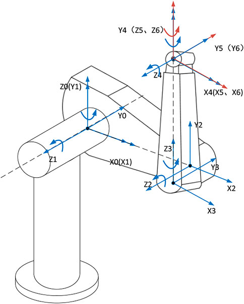
FIGURE 2. Transformation relationship of the coordinate system of each joint of the manipulator Puma 560.

TABLE 1

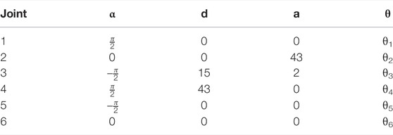
TABLE 1. DH model parameters of the manipulator Puma 560.

3.2.2 Collision Detection Model for Live Working Manipulator

Since most of the obstacles in the working environment of the live working manipulator should be wires, the obstacles are simplified as cylinders in this research. The obstacle avoidance of the manipulator, on the contrary, cannot be attributed just to the obstacle avoidance problem at the manipulator’s end-effector, and the obstacle avoidance of each manipulator’s link must also be considered. As a result, to solve the manipulator’s obstacle avoidance problem, geometric knowledge must be combined. This research employs the cylindrical to envelope links and obstacle, as illustrated in Figure 3.

FIGURE 3

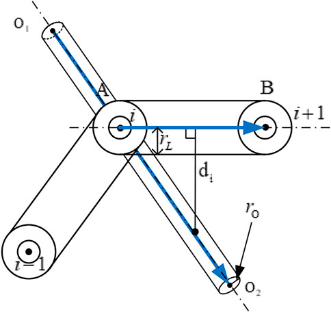
FIGURE 3. Schematic diagram of the manipulator obstacle avoidance detection model.

The link between the manipulator’s joints $i$ and $i+1$ is denoted by AB, $r_L$ is the radius of the radial surface of the cylindrical model of the enveloping manipulator, $O_1, O_2$ are the two endpoints of the obstacle model, and $r_O$ is the radial radius of $O_1{O}_2$, so whether the manipulator’s link AB is in contact with the obstacle can be expressed as

$d_i<r_L+r_O+r_{safe}(1)$

where $r_{safe}$ is the radius allowance to ensure safety and $d_i$ is the distance between the line segment AB and the line segment $O_1{O}_2$, which can be obtained by the following formula (Shen et al., 2015):

$d_i=\{\begin{array}{l}{\Vert \left(A+{\lambda }_1\overrightarrow{AB}\right)-\left(O_1+{\lambda }_2\overrightarrow{O_1{O}_2}\right)\Vert }_2,if 0\le {\lambda }_1,{\lambda }_2\le 1\\ \min \left( d\left(O_1,\overrightarrow{AB}\right), d\left(O_2,\overrightarrow{AB}\right) ,d\left(A,\overrightarrow{O_1{O}_2}\right) d\left(B,\overrightarrow{O_1{O}_2}\right)\right),else\end{array}(2)$

where

${\lambda }_1=\frac{\left(\overrightarrow{AB}\cdot \overrightarrow{O_1{O}_2}\right)(\overrightarrow{A{O}_1}\cdot \overrightarrow{O_1{O}_2})-{\left(\overrightarrow{O_1{O}_2}\right)}^2\overrightarrow{A{O}_1}\cdot \overrightarrow{AB}}{{\left(\overrightarrow{AB}\right)}^2{\left(\overrightarrow{O_1{O}_2}\right)}^2-{\left(\overrightarrow{AB}\cdot \overrightarrow{O_1{O}_2}\right)}^2},$

${\lambda }_2=-\frac{\left(\overrightarrow{AB}\cdot \overrightarrow{O_1{O}_2}\right)(\overrightarrow{A{O}_1}\cdot \overrightarrow{AB})-{\left(\overrightarrow{AB}\right)}^2\overrightarrow{A{O}_1}\cdot \overrightarrow{O_1{O}_2}}{{\left(\overrightarrow{AB}\right)}^2{\left(\overrightarrow{O_1{O}_2}\right)}^2-{\left(\overrightarrow{AB}\cdot \overrightarrow{O_1{O}_2}\right)}^2},$

$d\left(O_1,\overrightarrow{AB}\right)$ is the distance from point $O_1$ to line segment AB, which can be calculated as

$d\left(O_1,\overrightarrow{AB}\right)=\{\begin{array}{c}\frac{{\Vert \overrightarrow{AB}\times \overrightarrow{A{O}_1}\Vert }_2}{{\Vert \overrightarrow{AB}\Vert }_2}, if 0\le \frac{\overrightarrow{A{O}_1}\cdot \overrightarrow{AB}}{{\overrightarrow{AB}}^2}\le 1\\ \min \left(\left|\overrightarrow{A{O}_1}\right|,\left|\overrightarrow{B{O}_1}\right|\right), else\end{array}$

and $d\left(O_2,\overrightarrow{AB}\right),d\left(A,\overrightarrow{O_1{O}_2}\right),\text{and }d\left(B,\overrightarrow{O_1{O}_2}\right)$ are the same, in which

$A=\left[T_i\left[\mathrm{0,3}\right],T_i\left[\mathrm{1,3}\right],T_i\left[\mathrm{2,3}\right]\right],$

$B=\left[T_{i+1}\left[\mathrm{0,3}\right],T_{i+1}\left[\mathrm{1,3}\right],T_{i+1}\left[\mathrm{2,3}\right]\right].$

Here, $T_i$ and $T_{i+1}$ are the coordinates of the manipulator’s joint $i$ and joint $i+1$ relative to the base coordinate system, which are generally described as a $4\times 4$ matrix, as shown in the following equation:

$T=\left[\begin{array}{cc}\begin{array}{cc}{T}_{00}& T_{01}\\ T_{10}& T_{11}\end{array}& \begin{array}{cc}{T}_{02}& T_{03}\\ T_{12}& T_{13}\end{array}\\ \begin{array}{cc}{T}_{20}& T_{21}\\ 0& 0\end{array}& \begin{array}{cc}{T}_{22}& T_{23}\\ 0& 1\end{array}\end{array}\right](3)$

Here, $T_{00}$, $T_{01}$, $T_{02}$, $T_{10}$, $T_{11}$, $T_{12}$, $T_{20}$, $T_{21}$, $T_{22}$ describe the gesture and $T_{03}$, $T_{13}$, $T_{23}$ describe the location.

So, it can be determined whether the manipulator collides with the obstacle by finding out whether each link of the manipulator collides with the obstacle; that is,

$f_{ob}=1-{\mathrm{\Pi }}_{i=0}^6{f}_{ob}^i(4)$

Combining with Eq. 1, we define $f_{ob}^i$ as

$f_{ob}^i=\{\begin{array}{c}1, if d_i<r_L+r_O+r_{safe}\\ 0, else \end{array}(5)$

3.2.3 Manipulator Polynomial Trajectory Model

Since there are infinite solutions for the manipulator to reach the target point from the source point, this research establishes an ideal model of the manipulator’s motion trajectory. The trajectory model is set as a sextic polynomial in this research; that is,

$\theta \left(\text{t}\right)=a_0+a_{1}t+a_2{t}^2+a_3{t}^3+a_4{t}^4+a_5{t}^5+a_6{t}^6(6)$

Substituting the source point and the set intermediate point, we can get

$\begin{array}{c}\text{θ}\left(0\right)={\text{a}}_0,\\ \begin{array}{c}\dot{\theta }\left(0\right)=a_1,\\ \begin{array}{c}\ddot{\theta }\left(0\right)=2a_2,\\ \begin{array}{c}\theta \left(T_1\right)=a_0+a_1{T}_1+a_2{T}_1^2+a_3{T}_1^3+a_4{T}_1^4+a_5{T}_1^5+a_6{T}_1^6,\\ \begin{array}{c}\dot{\theta }\left(T_1\right)=a_1+2a_2{T}_1+3a_3{T}_1^2+4a_4{T}_1^3+5a_5{T}_1^4+6a_6{T}_1^5,\\ \ddot{\theta }\left(T_1\right)=2a_2+6a_3{T}_1+12a_4{T}_1^2+20a_5{T}_1^3+30a_6{T}_1^4.\end{array}\end{array}\end{array}\end{array}\end{array}(7)$

Here, $\theta \left(0\right)$, $\dot{\theta }\left(0\right)$, $\ddot{\theta }\left(0\right)$ are the joint angle, angular velocity, and angular acceleration at the source point of the manipulator, $T_1$ is the running time of the trajectory, and $\theta \left(T_1\right), \dot{\theta }\left(T_1\right),\ddot{ \theta }\left(T_1\right)$ are the joint angle, angular velocity, and angular acceleration of the goal point. Taking $a_6$ and $T_1$ as known conditions, we can get $a_0\sim a_5$ as follows:

$\begin{array}{c}{a}_0=\text{θ}\left(0\right),\\ \begin{array}{c}{a}_1=\dot{\theta }\left(0\right),\\ \begin{array}{c}{a}_2=\frac{\ddot{\theta }\left(0\right)}{2},\\ a_3=-\begin{array}{c}\frac{20\theta \left(0\right)-20\theta \left(T_1\right)+8\dot{\theta }\left(T_1\right)T_1+12\dot{\theta }\left(0\right)T_1+2a_6{T}_1^6-\ddot{\theta }\left(T_1\right)T_1^2+3T_1^2\ddot{\theta }\left(0\right)}{2T_1^3},\\ a_4=\begin{array}{c}\frac{30\theta \left(0\right)-30\theta \left(T_1\right)+7\dot{\theta }\left(T_1\right)T_1+16\dot{\theta }\left(0\right)T_1+6a_6{T}_1^6-2\ddot{\theta }\left(T_1\right)T_1^2+3T_1^2\ddot{\theta }\left(0\right)}{2T_1^4},\\ a_5=-\begin{array}{c}\frac{12\theta \left(0\right)-12\theta \left(T_1\right)+6\dot{\theta }\left(T_1\right)T_1+6\dot{\theta }\left(0\right)T_1+6a_6{T}_1^6-\ddot{\theta }\left(T_1\right)T_1^2+T_1^2\ddot{\theta }\left(0\right)}{2T_1^5}.\end{array}\end{array}\end{array}\end{array}\end{array}\end{array}(8)$

The joint angle of the source point and the target point are known conditions, angular velocity, and angular acceleration of the source point, and the target point is always set at 0. So, parameters $a_6$ and $T_1$ are the seven parameters that the algorithm needs to optimize.

3.2.4 Optimizing Parameters of the Trajectory Model Using PSO

According to Definition 1 and Eq. 4, it is evident that the manipulator motion planning problem can be considered a multi-objective optimization problem, that is,

$\begin{array}{c}\mathit{min} f\left(x\right)=\left[\text{Δ}{\theta }_i\left(x\right), \text{Δ}L\left(x\right)\right],i=\mathrm{1,2}, \dots ,6,\\ s.t. d_i\left(x\right)>r_L+r_O+r_{safe}, i=\mathrm{1,2}, \dots ,6,\end{array}(9)$

where $\text{Δ}{\theta }_i\left(x\right)$ is the cumulative rotation change of joint $i$ from the source point to the target point and $\text{Δ}L\left(x\right)$ is the cumulative movement change of the manipulator’s end-effector from the source point to the target point. The constraint condition is that each link of the manipulator can avoid obstacles.

$x$ is the parameter in the manipulator’s motion trajectory model, which includes the seven parameters listed in Section 3.2.3. This problem does not require the optimization of controller settings; instead, just the proposed model parameters must be optimized. The PSO algorithm is utilized to optimize the parameters in this work, which is a relatively developed algorithm. The fitness function designed in this research is

$f=-\frac{f_{ob}}{{\eta }_1{{\displaystyle \sum }}_{i=1}^6\text{Δ}{\theta }_i+{\eta }_2\text{Δ}L}(10)$

where $f_{ob}$ estimates whether each link of the manipulator collides with the obstacle, whose value is obtained from Eq. 4. The parameters ${\eta }_1$ and ${\eta }_2$ are used to balance the cumulative changes in joint angle and end-effector movement, respectively. The interpolation approach is employed to derive $\text{Δ}{\theta }_i$ and $\text{Δ}L$ in this study since the beginning point to the goal location is a continuous trajectory.

3.3 Data-Driven Part Design

3.3.1 Markov Modeling Process

For the motion planning problem of the manipulator, it is difficult to obtain the complete state of the manipulator, so this problem is a partially observable Markov decision process (POMDP). Define the Markov decision process $M=<S,A,P,R ,\gamma >$, where γ is the discount coefficient, which is determined manually. The following describes S, A, P, and R, respectively:

1) Design of the state space. To improve the generalization performance of the algorithm, we take the current joint angle $q^i\in q, i=\mathrm{1,2},\dots ,6 , -2\pi \le q^i\le 2\pi$, the joint angle at last moment $q_l^i\in q_l, i=\mathrm{1,2},\dots ,6 , -2\pi \le q_l^i\le 2\pi$, and the target joint angle $q_g^i\in q_g, i=\mathrm{1,2},\dots ,6 , -2\pi \le q_g^i\le 2\pi$, of the manipulator as part of the state. At the same time, in order to avoid obstacles, we also take the distance of each link of the manipulator relative to the obstacle $d_{t0-ob}^i\in d_{to-ob},d_{last-t0-ob}^i\in d_{last-to-ob},i=\mathrm{1,2},\dots ,6$, as part of the state, and then the complete state is

$S=<q,q_l,q_g,d,d_l>(11)$

2) Design of the action space. The motion increment of each joint angle of the manipulator is the algorithm’s output action in manipulator motion planning. As a result, the action proposed in this work is the angle increment of the manipulator’s six joints $\text{Δ}{q}^i,i=\mathrm{1,2},\dots ,6$.

3) State transition. This work introduces the action scaling parameter ${\alpha }_s$ to ensure motion continuity and reason; then,

$q=q+{\alpha }_s\text{Δ}q(12)$

4) Design of reward function. The problem in this research is very complex, there is only a direct relationship with the action $\text{Δ}q$ in the state space, and additional information and actions in the state space are only indirectly related. For reward function design, see Section 3.3.2 for details.

3.3.2 D-SAC Algorithm

As shown in Figure 4, when the manipulator learns by interacting with the environment, in order to avoid obstacles and reach the target point, the training process is actually the process of learning the kinematics model of the robotic arm and the obstacle avoidance detection model.

FIGURE 4

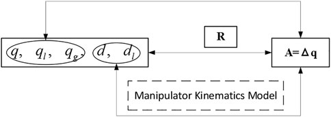
FIGURE 4. State space and action space.

Simple sparse rewards make it difficult for the manipulator to successfully complete the task and get a positive reward under the simple sparse reward conditions, making learning easy to fall into the local optimum (the manipulator collides with the obstacle). So, the D-SAC algorithm is proposed in this research. The reward function designed in D-SAC is as follows:

$R=\{\begin{array}{c}{R}_{suc}, {\mathrm{\Vert q\Vert }}_2<\epsilon \\ R_{out}, -2\pi <q+q_{target}<2\pi \\ R_{ob},f_{ob}=0 \\ R_o, else \end{array}(13)$

where $R_{suc}$ is the reward of the manipulator successfully reaching the target point. The judgment condition for the manipulator successfully reaching the target point is that the error of the current joint angle and the target joint angle is within the allowable error $\epsilon$. $R_{out}$ is the penalty for the current joint angle of the manipulator exceeding the working range of the manipulator, and $R_{ob}$ is the penalty for the manipulator hitting an obstacle, and its value can be obtained from Eq. 4. $R_o$ is the reward of the manipulator under general conditions, including two parts: target guidance and fixed penalty:

$R_o={\alpha }_1{r}_q+\left(1-\left[{\alpha }_1{r}_q\right]\right)\cdot r^{-}(14)$

where $r^{-}$ is a fixed penalty term and the function $\left[x\right]$ is a truth function. When $x$ is 0, the function value is 0; otherwise, it is 1.

Target guidance item $r_q$. It is easy to think of utilizing the Euclidean norm of the current joint angle as the measurement standard for the target guidance item, but merely using the Euclidean norm as the reward function’s design parameter is extremely likely to be ineffective. It may make the manipulator travel back and forth at some useless positions in order to gain a bigger cumulative reward, as shown in Figure 5A, which is termed the manipulator’s back-and-forth dilemma in this research.

FIGURE 5

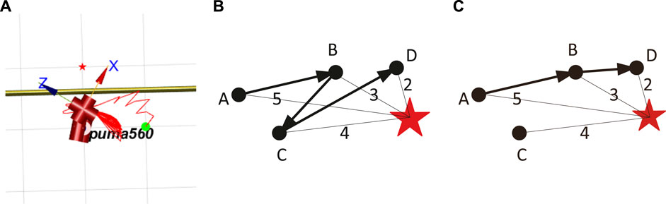
FIGURE 5. Back-and-forth dilemma. (A) Back-and-forth dilemma of the manipulator. (B) Simulation 1st of back-and-forth dilemma. (C) Simulation 2nd of back-and-forth dilemma.

Definition 2: The back-and-forth dilemma: the manipulator moves repeatedly in certain positions in order to get a larger cumulative reward.

It would be better to calculate the difference between the current joint angle’s Euclidean norm and the last joint angle’s Euclidean norm:

$r_q=\Vert q_l-q_g\Vert 2-\Vert q-q_g\Vert 2(15)$

However, the reward function of Eq. 15 cannot avoid the manipulator’s back-and-forth dilemma. The following uses a 2D space as an example to prove this. The joint angle space of the manipulator is 6D, but the reason is the same.

As shown in Figures 5B,C, the distances from point A, point B, point C, and point D to the target point are 5, 3, 4, and 2. When the manipulator moves according to the trajectory shown in Figure 5B, the cumulative reward obtained during this period is $r_1=\left(5-3\right)+\left(3-4\right)+\left(4-2\right)=3$. When the manipulator moves according to the trajectory shown in Figure 5C, the cumulative reward obtained during this period is $r_2=\left(5-3\right)+(3-2)$. $r_1=r_2$. So if the reward function is designed in this way, the manipulator still cannot avoid the back-and-forth dilemma.

Therefore, to avoid the back-and-forth dilemma, we introduce the guiding coefficient ${\alpha }_1$. Inspired by Coulomb’s law, the setting of the coefficient ${\alpha }_1$ takes into account that the closer the robot arm is to the target point, the greater the attractive force is. At the same time, to avoid too large or too small coefficients, this study scales $q$ to the range of 0.08–1.0. The target guidance coefficient is set as shown in the following equation:

${\alpha }_1^i=\frac{5}{clip\left(q^i, 0.08,1\right)},i=\mathrm{1,2}, \dots ,6(18)$

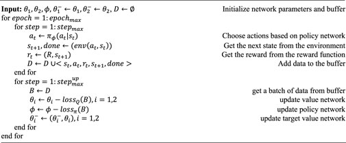
In summary, the process of the D-SAC algorithm is as follows (for the meaning of relevant parameters, refer to Table 2).

TABLE 2

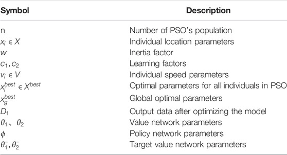
TABLE 2. Symbol description table of P-SAC.

Algorithm 1. D-SAC algorithm.

3.4 P-SAC Algorithm Driven by Hybrid Data Model

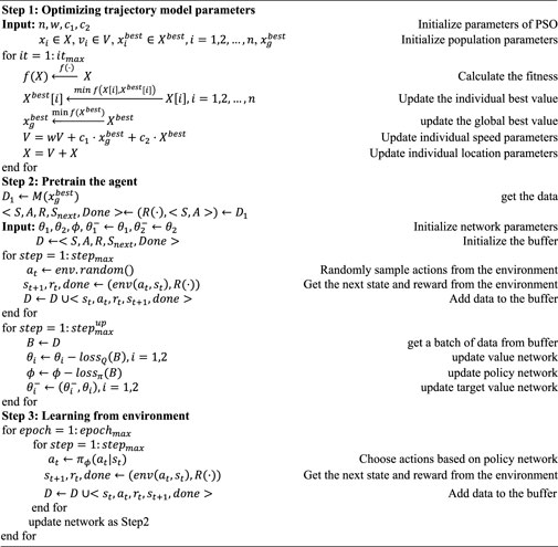
To summarize, this research proposes P-SAC, a fusion algorithm of PSO and SAC for the live working manipulator’s motion planning, based on the proposed algorithm framework, which is driven by data and model. The algorithm is broken into the following three sections:

Step 1: Optimize the model’s parameters. Establish the $\mathrm{ℳ}$ set of models based on the manipulator’s DH model, obstacle avoidance detection model, and polynomial trajectory model. Using the PSO algorithm to optimize the parameters of M, the parameters to be optimized here are the seven parameters described in Section 3.2.3.

Step 2: Pre-train the agent. The dataset $D_1$ is obtained using the trajectory model optimized by Step 1, the state value and action value $<S,A>$ are retrieved from the dataset $D_1$, and $<S,A>$ are translated into $<S,A,R,S_{-},D>$ using the reward function. To update the agent’s network parameters, enter $<S,A,R,S\_,D>$ into the buffer.

Step 3: Learn from the environment. Interactive learning between the agent obtained by pre-training in Step 2 and the environment improves the robustness of the algorithm.

The P-SAC algorithm flow is as follows (for the meaning of relevant parameters, refer to Table 2).

Algorithm 2. : P-SAC algorithm.

4 Experimental Results and Analysis

4.1 Simulation Experiment Verification

The architecture diagram of P-SAC applied to the live working manipulator is shown in Figure 6.

FIGURE 6

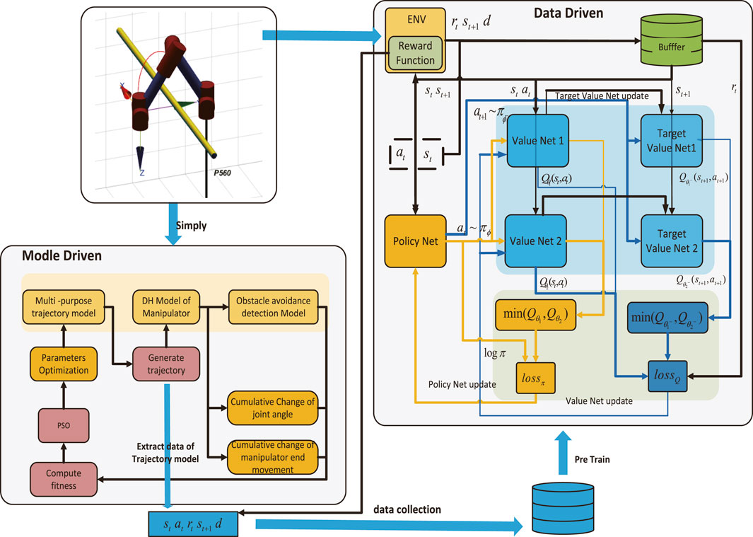
FIGURE 6. Architecture diagram of P-SAC applied to the live working manipulator.

In this research, Robotics Toolbox is used to model a six-DOF live working manipulator to verify the algorithm. The experimental software and hardware environment is shown in Table 3.

TABLE 3

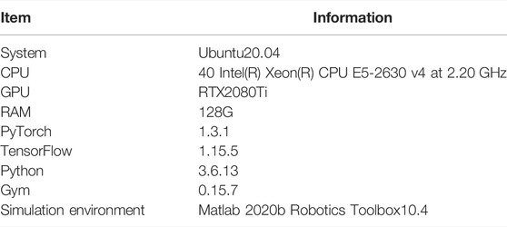
TABLE 3. Environment of experimental software and hardware.

The source point of the joint of the manipulator is $\left[2.8369, 2.1575, 0.4422, 0, 0.5419,-0.\mathrm{3047}\right]$, and the target point of the joint is $\left[4.4077, 2.1575, 0.4422, 0, 0.5419, 1.2661\right]$. So, the source point and target point of the manipulator end-effector are $\left[\mathrm{50,0,0}\right]$ and $\left[0, 50, 0\right]$. The starting point and ending point of the cylindrical obstacle are $\left[-\mathrm{100,30,10}\right]$ and $\left[\mathrm{100,30,10}\right]$, and the obstacle radius is 3. The parameters used in the P-SAC algorithm in this paper are shown in Table 4.

TABLE 4

TABLE 4. Algorithm hyperparameters.

4.2 Analysis of Results

The reward curves of D-SAC and P-SAC applied in the live working manipulator are shown in Figure 7. The reward values for the final convergence of P-SAC and D-SAC are shown in Table 5. It is evident that P-SAC reaches the convergence state earlier, and its final convergence value is higher than that of D-SAC. It is evident from the curve that P-SAC reaches near the optimal value earlier but begins to decrease after a period of time and finally rises to the optimal value. This shows that the initial pre-training of the P-SAC algorithm lets the agent acquire a certain ability to learn about the environment, but then it starts to learn what actions are bad in the process of interacting with the environment, which leads to a decrease in the reward value.

FIGURE 7

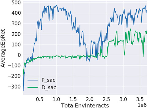
FIGURE 7. Average epoch reward curves of D-SAC and P-SAC.

TABLE 5

TABLE 5. Final convergence value of D-SAC and P-SAC.

The motion process of P-SAC, D-SAC, and PSO is shown in Figure 8. It is evident that all three algorithms can effectively avoid obstacles.

FIGURE 8

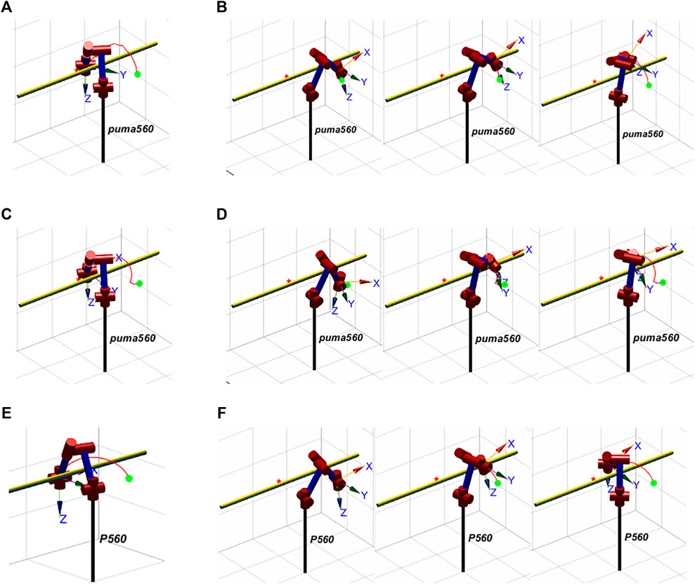
FIGURE 8. Process of manipulator’s motion. (A) Complete motion trajectory of D-SAC. (B) Obstacle avoidance process of D-SAC. (C) Complete motion trajectory of P-SAC. (D) Obstacle avoidance process of P-SAC. (E) Complete motion trajectory of PSO. (F) Obstacle avoidance process of PSO.

The curves of each joint angle of the manipulators using P-SAC, D-SAC, and PSO with time are shown in Figure 9. The joint angle change curves of P-SAC and D-SAC are relatively smooth, but there is a certain gap compared with the joint angle change of the PSO algorithm, especially for D-SAC, and it is evident that the curve has obvious jitter. Since PSO pre-plans a perfect trajectory, its curve must be extremely smooth, while D-SAC and GP-SAC are real-time changing curves, so the curves are not so perfect. However, there is no sudden change in its curve, and it is enough for the manipulator to work effectively.

FIGURE 9

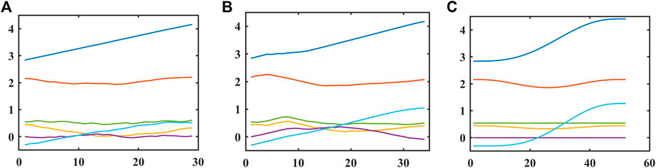
FIGURE 9. Change curve of the angle of each joint of the manipulator. (A) D-SAC. (B) P-SAC. (C) PSO.

In conclusion, using P-SAC proposed in this paper can effectively improve the training efficiency of the data-driven algorithm and can complete the real-time motion planning of the live working manipulator.

5 Conclusion

Aiming at the shortcomings of data-driven algorithms represented by deep reinforcement learning, which take too long in the early stage of training, and model-driven algorithms that have poor generalization ability to environmental changes and cannot avoid model design errors, this study proposes a hybrid data-model–driven algorithm framework. Under this framework, this study proposes the P-SAC algorithm that integrates PSO and reinforcement learning and applies the P-SAC algorithm to the motion planning problem of live working manipulators. The experimental results show that the proposed P-SAC algorithm has a faster convergence rate than the SAC algorithm, reduces the training time, and can better adapt to the changing environment than the model-driven algorithm.

The hybrid data-model–driven algorithm proposed in this paper can be applied to control problems with controllers or planning problems without controllers and has good application value and algorithm versatility.

Data Availability Statement

The original contributions presented in the study are included in the article/Supplementary Material, and further inquiries can be directed to the corresponding author.

Author Contributions

This is a joint work, and the authors were in charge of their expertise and capability. All authors participated in the design of the algorithm framework and algorithm process. TK was in charge of analysis, model design, and revision. JLi was in charge of writing, methodology validation and revision; JLiu was in charge of validation and revision; YL was in charge of data analysis. XL was in charge of manuscript revision.

Funding

This work was supposed by the National Key Research and Development Program of China under Grant 2020YFB1708503.

Conflict of Interest

The authors declare that the research was conducted in the absence of any commercial or financial relationships that could be construed as a potential conflict of interest.

Publisher’s Note

All claims expressed in this article are solely those of the authors and do not necessarily represent those of their affiliated organizations, or those of the publisher, the editors, and the reviewers. Any product that may be evaluated in this article, or claim that may be made by its manufacturer, is not guaranteed or endorsed by the publisher.

References

Cao, X., Zou, X., Jia, C., Chen, M., and Zeng, Z. (2019). RRT-based Path Planning for an Intelligent Litchi-Picking Manipulator. Comput. Electron. Agric. 156, 105–118. doi:10.1016/j.compag.2018.10.031

CrossRef Full Text | Google Scholar

Choset, H., Lynch, K. M., Hutchinson, S., Kantor, G. A., and Burgard, W. (2005). Principles of Robot Motion: Theory, Algorithms, and Implementations. Cambridge, MA, USA: MIT Press.

Google Scholar

Clavera, I., Held, D., and Abbeel, P. (2017). “Policy Transfer via Modularity and Reward Guiding,” in 2017 IEEE/RSJ International Conference on Intelligent Robots and Systems (IROS) (Vancouver, BC, Canada: IEEE Press), 1537–1544. doi:10.1109/IROS.2017.8205959

CrossRef Full Text | Google Scholar

Denavit, J., and Hartenberg, R. S. (2021). A Kinematic Notation for Lower-Pair Mechanisms Based on Matrices. J. Appl. Mech. 22 (2), 215–221. doi:10.1115/1.4011045

CrossRef Full Text | Google Scholar

Devlin, J., Chang, M., Lee, K., and Toutanova, K. (2019). “BERT: Pre-training of Deep Bidirectional Transformers for Language Understanding,” in Proceedings of the 2019 Conference of the North American Chapter of the Association for Computational Linguistics: Human Language Technologies. Minneapolis, Minnesota: Association for Computational Linguistics. Long and Short Papers 1, 4171–4186. doi:10.18653/v1/N19-1423

CrossRef Full Text | Google Scholar

Gasparetto, A., Boscariol, P., Lanzutti, A., and Vidoni, R. (2015). “Path Planning and Trajectory Planning Algorithms: A General Overview,” in Motion and Operation Planning of Robotic Systems. Editors G. Carbone, and G. B. Fernando (Cham: Springer International Publishing), 29, 3–27. Mechanisms and Machine Science. doi:10.1007/978-3-319-14705-5_1

CrossRef Full Text | Google Scholar

Gasparetto, A., Boscariol, P., Lanzutti, A., and Vidoni, R. (2012). Trajectory Planning in Robotics. Math. Comput. Sci. 6 (3), 269–279. doi:10.1007/s11786-012-0123-8

CrossRef Full Text | Google Scholar

Haarnoja, T., Zhou, A., Abbeel, P., and Levine, S. (2018). “Soft Actor-Critic: Off-Policy Maximum Entropy Deep Reinforcement Learning with a Stochastic Actor,” in Proceedings of the 35th International Conference on Machine Learning (PMLR), 1861–1870. Available at: https://proceedings.mlr.press/v80/haarnoja18b.html (Accessed July 13, 2022).

Google Scholar

Haarnoja, T., Zhou, A., Hartikainen, K., Tucker, G., Ha, S., Tan, J., et al. (2019). Soft Actor-Critic Algorithms and Applications. ArXiv. 1812.05905 [Cs, Stat]. doi:10.48550/arXiv.1812.05905

CrossRef Full Text | Google Scholar

Hao, D., Li, S., Yang, J., Wang, J., and Duan, Z. (2022). Research Progress of Robot Motion Control Based on Deep Reinforcement Learning. Control Decis. 37 (02), 278–292. doi:10.13195/j.kzyjc.2020.1382

CrossRef Full Text | Google Scholar

Holland, J. H. (1992). Adaptation in Natural and Artificial Systems: An Introductory Analysis with Applications to Biology, Control, and Artificial Intelligence. Cambridge, MA, USA: MIT Press.

Google Scholar

Kalashnikov, D., Irpan, A., Pastor, P., Ibarz, J., Herzog, A., Jang, E., et al. (2018). QT-opt: Scalable Deep Reinforcement Learning for Vision-Based Robotic Manipulation. ArXiv. 1806.10293 [Cs, Stat]. doi:10.48550/arXiv.1806.10293

CrossRef Full Text | Google Scholar

Kennedy, J., and Eberhart, R. (1995). “Particle Swarm Optimization,” in Proceedings of ICNN’95 - International Conference on Neural Networks (Perth, WA, Australia: IEEE Press), 1942–1948. doi:10.1109/ICNN.1995.4889684

CrossRef Full Text | Google Scholar

Khatib, O. (1985). Real-Time Obstacle Avoidance for Manipulators and Mobile Robots. IEEE Int. Conf. Robotics Automation Proc. 2, 500–505. doi:10.1109/ROBOT.1985.1087247

CrossRef Full Text | Google Scholar

Krizhevsky, A., Sutskever, I., and Hinton, G. E. (2017). ImageNet Classification with Deep Convolutional Neural Networks. Commun. ACM 60 (6), 84–90. doi:10.1145/3065386

CrossRef Full Text | Google Scholar

Lillicrap, T. P., Hunt, J. J., Pritzel, A., Heess, N. M., Erez, T., Tassa, Y., et al. (2019). “Continuous Control with Deep Reinforcement Learning,” in 4th International Conference on Learning Representations (ICLR), San Juan, Puerto Rico, May 2–4, 2016. Available at: https://dblp.org/rec/journals/corr/LillicrapHPHETS15.bib.

Google Scholar

Lynch, K. M., and Park, F. C. (2017). Modern Robotics: Mechanics, Planning, and Control. Cambridge, UK: Cambridge University Press.

Google Scholar

Ma, L., Cheng, S., and Shi, Y. (2021c). Enhancing Learning Efficiency of Brain Storm Optimization via Orthogonal Learning Design. IEEE Trans. Syst. Man. Cybern. Syst. 51 (11), 6723–6742. doi:10.1109/TSMC.2020.2963943

CrossRef Full Text | Google Scholar

Ma, L., Huang, M., Yang, S., Wang, R., and Wang, X. (2021a). An Adaptive Localized Decision Variable Analysis Approach to Large-Scale Multiobjective and Many-Objective Optimization. IEEE Trans. Cybern. 99, 1–13. doi:10.1109/TCYB.2020.3041212

CrossRef Full Text | Google Scholar

Ma, L., Li, N., Guo, Y., Wang, X., Yang, S., Huang, M., et al. (2021b). Learning to Optimize: Reference Vector Reinforcement Learning Adaption to Constrained Many-Objective Optimization of Industrial Copper Burdening System. IEEE Trans. Cybern., 1–14. doi:10.1109/TCYB.2021.3086501

CrossRef Full Text | Google Scholar

Ma, L., Wang, X., Wang, X., Wang, L., Shi, Y., and Huang, M. (2021d). TCDA: Truthful Combinatorial Double Auctions for Mobile Edge Computing in Industrial Internet of Things. IEEE Trans. Mob. Comput., 1. doi:10.1109/TMC.2021.3064314

CrossRef Full Text | Google Scholar

Menendez, O., Auat Cheein, F. A., Perez, M., and Kouro, S. (2017). Robotics in Power Systems: Enabling a More Reliable and Safe Grid. EEE Ind. Electron. Mag. 11 (2), 22–34. doi:10.1109/MIE.2017.2686458

CrossRef Full Text | Google Scholar

Mnih, V., Kavukcuoglu, K., Silver, D., Graves, A., Antonoglou, I., Wierstra, D., et al. (2013). Playing Atari with Deep Reinforcement Learning. ArXiv. 1312.5602 [Cs, Stat], 9. doi:10.48550/arXiv.1312.5602

CrossRef Full Text | Google Scholar

Rulong, Q., and Wang, T. (2014). An Obstacle Avoidance Trajectory Planning Scheme for Space Manipulators Based on Genetic Algorithm. ROBOT 36 (03), 263–270. doi:10.3724/SP.J.1218.2014.00263

CrossRef Full Text | Google Scholar

Shen, Y., Jia, Q., Chen, G., Wang, Y., and Sun, H. (2015). “Study of Rapid Collision Detection Algorithm for Manipulator,” in 2015 IEEE 10th Conference on Industrial Electronics and Applications (ICIEA) (Auckland, New Zealand: IEEE), 934–938. doi:10.1109/ICIEA.2015.7334244

CrossRef Full Text | Google Scholar

Shi, Y. (2011). “Brain Storm Optimization Algorithm,” in Advances in Swarm Intelligence. Editors Y. Tan, Y. Shi, Y. Chai, and G. Wang (Berlin, Heidelberg: Springer), 303–309. Lecture Notes in Computer Science. doi:10.1007/978-3-642-21515-5_36

CrossRef Full Text | Google Scholar

Siciliano B., Sciavicco L., Villani L., and Oriolo G. (Editors) (2009). “Motion Planning,” Robotics: Modelling, Planning and Control (London: Springer), 523–559. doi:10.1007/978-1-84628-642-1_12

CrossRef Full Text | Google Scholar

Wang, M., Luo, J., and Walter, U. (2015). Trajectory Planning of Free-Floating Space Robot Using Particle Swarm Optimization (PSO). Acta Astronaut. 112, 77–88. doi:10.1016/j.actaastro.2015.03.008

CrossRef Full Text | Google Scholar

Wei, K., and Ren, B. (2018). A Method on Dynamic Path Planning for Robotic Manipulator Autonomous Obstacle Avoidance Based on an Improved RRT Algorithm. Sensors 18 (2), 571. doi:10.3390/s18020571

CrossRef Full Text | Google Scholar

Wu, Y.-H., Yu, Z.-C., Li, C.-Y., He, M.-J., Hua, B., and Chen, Z.-M. (2020). Reinforcement Learning in Dual-Arm Trajectory Planning for a Free-Floating Space Robot. Aerosp. Sci. Technol. 98, 105657. doi:10.1016/j.ast.2019.105657

CrossRef Full Text | Google Scholar

Yang, Q., Ku, T., and Hu, K. (2021). Efficient Attention Pyramid Network for Semantic Segmentation. IEEE Access 9, 18867–18875. doi:10.1109/ACCESS.2021.3053316

CrossRef Full Text | Google Scholar

Yu, N., Nan, L., and Ku, T. (2021). Multipolicy Robot-Following Model Based on Reinforcement Learning. Sci. Program. 2021, 8. doi:10.1155/2021/5692105

CrossRef Full Text | Google Scholar

Zhang, D., Han, X., Han, X., and Deng, C. (2018). Review on the Research and Practice of Deep Learning and Reinforcement Learning in Smart Grids. Csee Jpes 4 (3), 362–370. doi:10.17775/CSEEJPES.2018.00520

CrossRef Full Text | Google Scholar