Evaluation of fuel consumption and emissions benefits of connected and automated vehicles in mixed traffic flow

1 Introduction

Global climate change and energy crisis are increasingly attracting people’s attention (Gov, 2018), and the transportation is an important factor leading to energy consumption and carbon emissions (Li et al., 2023). Recent years, China’s car ownership has grown rapidly and has raised concerns about sustainable energy, transportation safety and climate change. According to statistics, China’s reliance on oil importation exceeded 65 percent by the end of 2017 (Gov, 2018). Meanwhile, the transportation accounts for a large share of the greenhouse gas (GHG) emissions. In response to the environmental crisis, government has introduced policies to encourage people to buy new energy vehicles instead of fuel vehicles to achieve energy saving and emission reduction. However, in the 2012–2020 Energy Conservation and New Energy Vehicle Industry Development Plan (China, 2018), the total production and sales of electric CAVs and hybrid (fuel-aided) vehicles are expected to reach 5 million units by 2020, which is more than five times of the current holdings (Xiong et al., 2019).

Meanwhile, the annual growth rate of GHG emissions from the transportationsector is higher than that of other shares (such as electricity, industry, agriculture, and commerce). It is expected that the annual emission of GHG from transportation will double by 2050 (Lamb et al., 2021). Within the transportation system, road-based travel is responsible for the most significant proportion of carbon emissions and energy consumption compared to other modes of transportation, such as aviation, rail, and marine (Lu et al., 2020). Passenger cars, light-duty trucks (including sport utility vehicles, pickup trucks, and minivans), and freight trucks emitted 41.6%, 18.0%, and 22.9%, respectively, of total United States transportation-sector GHG emissions in 2016 (Zong, 2019). In addition, the United States consumed approximately 143 billion gallons of motor gasoline, with a daily average of 391 million gallons in 2018 (Yao et al., 2021). Therefore, it can significantly reduce the energy consumption and carbon emissions of transportation systems by reducing vehicle fuel consumption and exhaust emissions, thereby alleviating the current issues of the global energy crisis and climate change.

The rapid growth in the number of vehicles is the main reason for the continuous increase in fuel consumption and exhaust emissions, and the traffic congestion caused by the increase in the number of vehicles has further increased fuel consumption and exhaust emissions (Romero and Gramkow, 2021). Therefore, alleviating traffic congestion is an effective means to reduce vehicle fuel consumption and exhaust emissions. Till now, the connected and automated vehicle (CAV) can generally realize information interaction and cooperative driving between other vehicles while effectively reducing the response delay of vehicles and shortening the distance between vehicles. For instance, some studies have investigated the relations between CAVs’ applications and greenhouse gas emissions (Zong, 2019; Romero and Gramkow, 2021).

Regarding the latest surveys, most people hold positive attitudes toward the automated CAVs of their green effects, and it has already aroused people’s interest (Labanca and Bertoldi, 2018; Baumgartner et al., 2022). Therefore, a large number of studies have been conducted on the impact of CAV on driving safety, traffic efficiency, and the environment. The application of CAV has great potential to improve traffic efficiency, driving safety, and stability (Ye and Yamamoto, 2019). Scholars generally believe that CAV is expected to improve the overall traffic quality from the micro level of traffic flow and reduce fuel consumption and exhaust emissions by alleviating traffic congestion (Kopelias et al., 2020). Therefore, we assume that, in reality, citizens are leaning towards replacing fuel CAVs with green energy CAVs (electronic) in order to protect the green world. We will mainly focus on the research on the impact of CAV on the environment and summarizes and analyzes existing research on fuel consumption and exhaust emissions in this paper.

In terms of fuel consumption. Rios-Torres et al. (Rios-Torres and Malikopoulos, 2018) analyzed the impact of CAV on fuel consumption in confluence ramp scenarios under different traffic volumes and market penetration rates (MPRs). They found that fuel consumption can only be reduced in mixed traffic scenarios with low traffic volumes. Islam et al. (Islam et al., 2019) conducted a comprehensive analysis of the impact of fuel consumption under different CAV scenarios and found that with the popularization of CAV, the average fuel consumption of conventional powertrains and hybrid electric vehicles has decreased by 1.5% and 2.2%, respectively. Ma et al. (Ma et al., 2019) proposed an eco-drive algorithm for CAV fuel consumption optimization on rolling terrains. The test results indicated that the algorithm could save more than 20% of fuel consumption. Alvarez et al. (Alvarez et al., 2020) studied the extent to which CAV can potentially reduce the overall fuel consumption of road vehicles. They found that the ability to shape vehicle speed trajectories collaboratively plays a dominant role in reducing urban/suburban fuel consumption, while platooning plays a dominant role in influencing the attainable fuel savings on the highway. Zhao et al. (Zhao et al., 2022) studied the fuel consumption of mixed traffic flow with CAV under three typical traffic scenarios (a basic segment with bottleneck zone, ramp of the freeway, and signalized intersection) based on the simulation platform of Python and SUMO. They found that the advantages of CAV are more evident at signalized intersections, and when the MPR of CAV is 100%, fuel consumption can be reduced by 32%. Huang et al. (Huang et al., 2023) established a fuel consumption calculation model for mixed human-driven vehicle (HUD) and CAV scenarios. The results showed that under the four MPRs of 20%, 50%, 80%, and 100%, the fuel consumption of CAV decreased by 0.8%–5%, 1.9%–12.5%, 8.6%–12%, and 12.4%, respectively, and the reduction effect of CAV fuel consumption was negatively correlated with vehicle speed.

In terms of exhaust emissions, Qin et al. (Qin et al., 2018) conducted a numerical simulation of a CAV fleet on an on-ramp highway using a car-following model and assessed the impact of queue stability on exhaust emissions by calculating the stability of the fleet using transfer function theory. The results showed that improving queue stability can effectively reduce traffic emissions. McConky et al. (McConky and Rungta, 2019) proposed a coordinated heuristic method to reduce exhaust emissions by reducing traffic congestion of CAV vehicles. The research results of Tu et al. (Tu et al., 2019) indicated that with the popularization of CAV, the GHG emissions were significantly reduced, but the emissions of nitrogen oxides were increased. Oswald et al. (Oswald et al., 2019) compared the CO₂ emissions from real-world measurements with estimates based on MOVES vehicle emission models and estimates provided by the physical-based Comprehensive Modal Emissions Model (CMEM). The results showed that MOVES underestimated the benefits of applying CAV to reduce emissions, and CMEM provided more accurate emission estimates. Pribyl et al. (Pribyl et al., 2020) demonstrated that introducing CAV into traffic flow can make significant progress in achieving EU emissions targets. Even at low MPRs of CAV, applying CAVs on the road can reduce CO₂ emissions by 10%–19%. Cai et al. (Cai et al., 2021) defined a new green vehicle routing problem (VRP) for CAV and used vehicle speed as a decision variable for the VRP. In addition, a nonlinear mixed integer programming model was established for the VRP to meet the demand for CAV while minimizing carbon emissions.

In summary, scholars have studied the impact of CAVs on fuel consumption and exhaust emissions in transportation systems from various perspectives, however, there are still some issues that need to be further considered. Firstly, most studies analyzed the impact of the application of CAVs on fuel consumption or exhaust emissions separately, without discussing the correlation between both fuel consumption and exhaust emissions under the same scenario. Secondly, previous studies generally used intersections or highways as research scenarios. However, the changes in traffic volume and speed during different periods on urban roads have led to more complex road conditions in this scenario.

Therefore, aiming to evaluate the co-benefits of both fuel and emission, we investigated the effects of deploying more CAVs and the environmental results together while exploring the daily urban traffic scenarios, tested and compared using different fuel consumption and exhaust emissions, given that the people are tending to use more green energy to protect the green world. Meanwhile, this study will also explore the carbon emissions of pure electric vehicles and the environmental effects with respect to the speeds.

Our paper is organized as follows. The Simulation part, including the data collection, processing, and parameter calibration in SUMO, is presented following the introduction. Next is a case study, including the simulation scenarios, results, and discussions. Finally, the research findings and limitations are concluded.

2 Methods

2.1 Overall simulation process

In order to assess the potential fuel consumption and emissions benefits of CAVs, we initiated a simulation utilizing SUMO under different levels of market penetration rate (MPR). These MPRs were categorized into eleven groups, ranging from 0% to 100% in increments of 10%. Human-driven Vehicles (HDVs)the employed Intelligent Driver Model (IDM) as their car-following model, while CAVs employed Cooperative Adaptive Cruise Control (CACC). Our fuel consumption and emissions models were based on the default settings offered by SUMO, including indicators of PM, HC, CO₂, and CO.

To be specific, we used SUMO for our experiments and analysis because it is an extensive road traffic simulator, which allows researchers to build on realistic network topologies to create simulations of vehicle movements. Also, SUMO is an open-source spatially continuous road traffic simulator commonly used to test ITS, which includes components of road networks network and vehicle demand modeling (e.g., traffic lights, right-of-way rules, lane changes) as well as public transport and pedestrian components. In addition, it also provides several tools to generate traffic demands (e.g., DUArouter, MArouter, OD2trips, Randomtrips) (Barbecho Bautista et al., 2021).

To ensure a realistic representation of road networks and traffic data, we utilized simulations that span 1 km long, reflecting real-world conditions. Before initiating the simulation, we calibrated SUMO parameters to reflect real-world traffic flow. Our methodology also incorporated a traffic survey and parameter calibration method, based on processed data, for comprehensive analysis.

2.2 Data collection and processing

We conducted a traffic survey on Hexing Road, Harbin, China. It is an arterial road with significant traffic demands in Harbin. The traffic survey was conducted during the peak hour in the morning, and the data were collected by video (shown in Figure 1). The traffic flow data on the main road were selected in this paper because there is too much interference on the auxiliary road which may make vehicles run abnormally, such as manual tricycles, motorcycles and other vehicles with irregular movements.

FIGURE 1

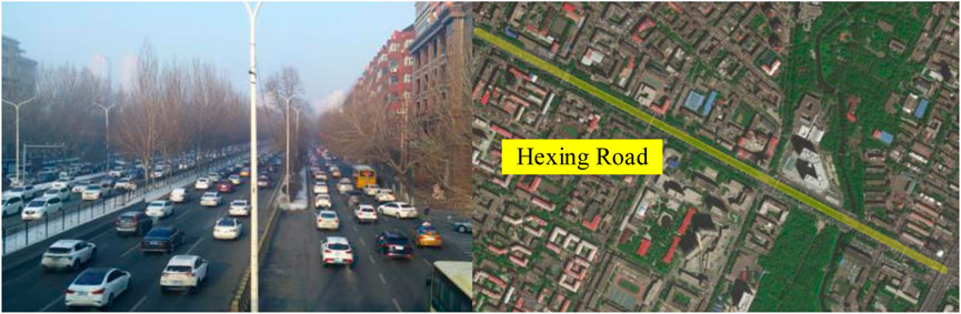
FIGURE 1. Location and reality of traffic survey.

The main road includes three lanes and the traffic volume is summarized in Table 1.

TABLE 1

TABLE 1. Statistics results of traffic volume.

Time headway and speed were extracted through the raw video data, and the detailed statistics of them were summarized in Table 2.

TABLE 2

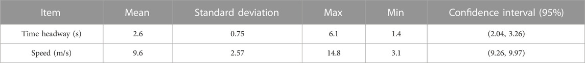
TABLE 2. Detailed statistics of time headway and speed.

A run test was conducted to verify if the statistics result of time headway was related to the sampling sequence. The run test result was summarized in Table 3, which found that the data was random. Simultaneously, the speed data was confirmed randomly by the run test (shown in Table 3).

TABLE 3

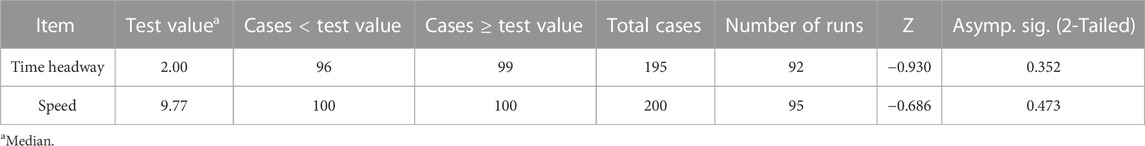
TABLE 3. Run test results of time headway and speed.

2.3 Parameter calibration

We conducted a sensitivity analysis to calibrate car-following model parameters, which include: acceleration (ACC), deceleration (DEC), max speed (SPE), time headway (TAU), and min gap (GAP). The general flow is illustrated in Figure 2.

FIGURE 2

FIGURE 2. The flow chart of the parameter calibration method.

Firstly, a benchmark value for each parameter was selected based on the average survey value or default value and expanded into a set of ten elements with the benchmark value as the center and an appropriate value as the step. This allowed each parameter to obtain a set of ten alternative values.

Secondly, a loop was set to traverse each candidate parameter. A KS test was conducted to verify if the simulated time headway and speed were non-significant differences compared to the real-world data (Wang et al., 2022). Furthermore, only when they both meet the requirements can it proceed to the next step. The statistic of the KS test can be calculated as follow:

$D=max\left|F_1\left(x\right)-F_2\left(x\right)\right|(1)$

where, $D$ is the statistic; $F_1\left(x\right)$ is the empirical distribution function of the real-world data about the observed value x; $F_2\left(x\right)$ is the empirical distribution function of the simulated data about the observed value x.

Finally, the simulated traffic needed to pass the GEH test. Precisely, it can be verified that the simulated traffic volume was non-significant different from the real world if the GEH is less than 5. The GEH value can be calculated as follow:

${GEH}_{ph}=\sqrt{\frac{{\left(Q_e-Q_s\right)}^2}{\left(Q_e+Q_s\right)/2}}(2)$

where, ${GEH}_{ph}$ is the GEH value during the peak hour between the real-world and simulation data; $Q_e$ is the real-world equivalent traffic volume, veh; $Q_s$ is the simulated traffic volume, veh.

The traffic flow characteristics of different roads are different, so we need to use the data in the real-world road traffic to calibrate some default parameters in SUMO, so that the traffic flow characteristics of the simulated roads in SUMO reflect those of the real-world roads, which makes it easy to compare and analyze. Then, the calibrated parameters are summarized in Table 4.

TABLE 4

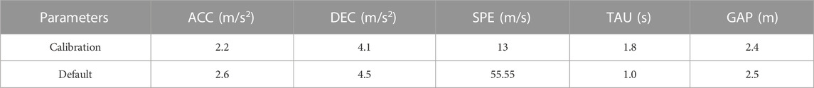
TABLE 4. The results of parameters calibration and the default in SUMO.

3 Results

3.1 Fuel consumption analysis

In this section, we aim to analyze the total fuel consumption on the road under different levels of MPR. By analyzing the fuel consumption by the vehicles through the simulation experiments, we can figure out the total energy waste and compare the enhancement after the intervention of the CAVs. In SUMO simulation, the measure of fuel consumption is by mg per unit. However, to unify units for subsequent comparison and analysis, we need to change the measure of fuel consumption to a liter per unit as follows:

$F_l=\frac{F_{mg}}{1\times {10}^6\bullet \rho }(3)$

where, $F_l$ is the fuel consumption, L/km or L/s; $F_{mg}$ is the fuel consumption, mg/km or mg/s; $\rho$ is the density of fuel, which is 0.7475 g/cm³, the average value of the gasoline in China.

Vehicles in Harbin are mainly fuel-driven vehicles, meanwhile, since our experiment is carried out with Hexing Road, which is the main road of the city and runs through the east and west of the city, the traffic flow characteristics are cyclical and representative. Therefore, converting the energy consumption of fuel vehicles into electricity consumption helps to compare better and analyze.

Afterward, we recorded the data of fuel consumption and the average speed of all vehicles on the road with different levels of MPR and compiled them into Figure 3. Generally, compared to 0 MPR, the fuel consumption under 50% MPR is reduced by 0.006 L/km or 5.1%. When MPR arrives at 100%, the fuel consumption is reduced by 0.0222 L/km or 18.0%. In addition to that, the average speed increased by 0.7 m/s (7.4%) from 0 MPR to 50% MPR. Moreover, the average speed increased by 3.0 m/s (31.6%) under 100% MPR compared with 0 MPR.

FIGURE 3

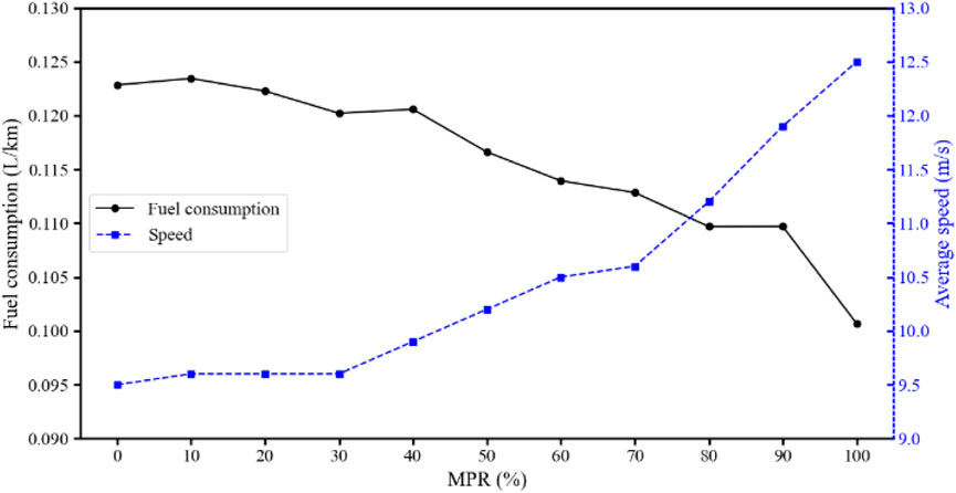
FIGURE 3. Fuel consumption and average speed under different MPRs.

On the other hand, as Figure 3 shows, with the increase of the MPRs, the fuel consumption of CAV is in a decreasing trend but also with a slight upward trend in several periods like 30%–40% MPR and 80%–90% MPR, while the average speed of each one is increasing in general but also with a stable period from 10% to 30% MPR.

3.2 Emissions analysis

In this section, we recorded data on the total emissions generated by traffic flow within the road per second and per vehicle per kilometer emissions under various MPRs for PM, HC, CO₂, and CO. The findings were presented as point-line and box-line plots in Figure 4. Our observations indicate that the overall emissions will decrease for all four indicators as the MPRs increase when looking at individual vehicles. For instance, PM emissions dropped from 0.23 mg/s to 0.14 mg/s when MPR increased to 100%. However, we also noted some phases of slightly increasing emissions per vehicle at MPRs between 30% to 40% and 80%–90% in the traffic flow.

FIGURE 4

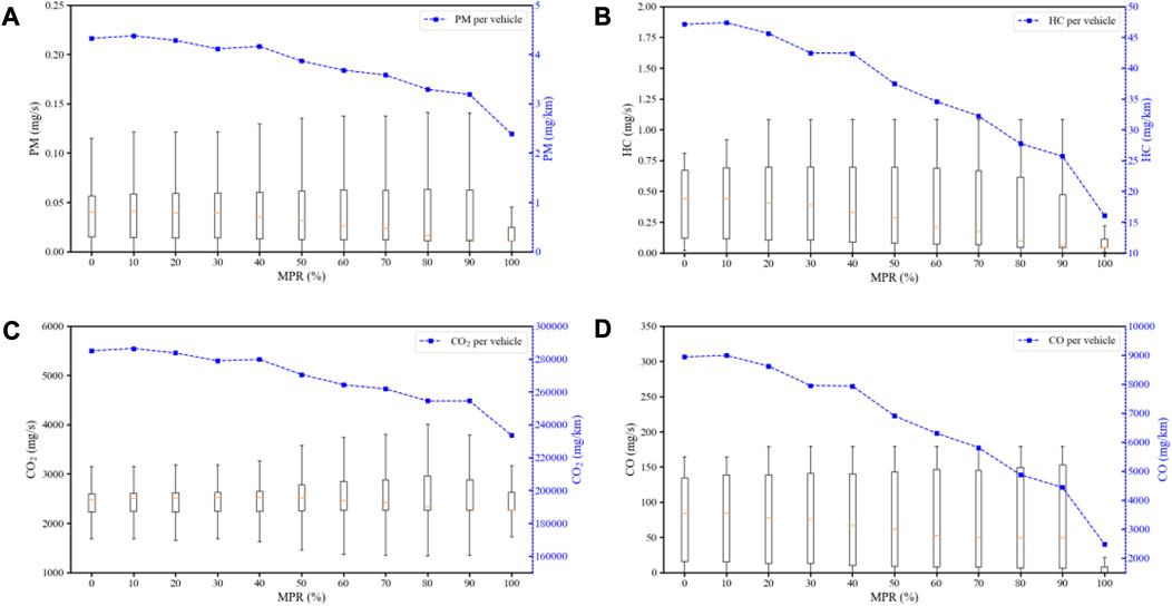
FIGURE 4. Emissions per second and kilometer under various MPRs. (A) PM emissions. (B) HC emissions. (C) CO₂ emissions. (D) CO emissions.

Furthermore, the box-line plots revealed a reduction in the median overall road emissions during a specific period with an increase in MPR. However, the range of emissions for each group of experiments gradually increased as MPR increased until the road was filled with CAVs until at the last period of 90%–100% MPR, it would suddenly fall. Similarly, the middle one-half of the data fluctuation interval for each group remained relatively constant until the road was filled with CAVs.

4 Discussion

4.1 Effect of low-speed vehicles

Low-speed vehicles in the traffic flow are one of the significant factors to influence road speed and overall emissions, and in this section, we focus on their impacts on the road and consider the road with mixed traffic flow. The mixed traffic flow generally contains HDVs and CAVs, as shown in Figure 5. In mixed traffic flows, low-speed vehicles will be taken into account, and they are usually treated as HDVs exclusively. In contrast, CAVs usually maintain safe and steady driving most of the time due to their excellent coordination and adaptation characteristics.

FIGURE 5

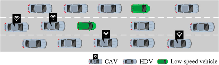
FIGURE 5. Mixed traffic flow with low-speed vehicles interference.

In the daily traffic flow on the roads, there are usually several reasons causing vehicles to maintain low speeds. First, most heavy vehicles, such as trucks and lorries, usually drive at lower speeds due to excessive load and their horsepower performance (Song and Yu, 2011). Secondly, some novice drivers will drive at low speeds due to their poor driving skills (Paul Anthikkat et al., 2013). The above two points are the main reasons for low-speed driving. In addition, a traffic accident on the road will cause most the vehicles to pass at a low speed, dramatically reducing the road’s average speed, causing traffic congestion, and increasing overall vehicle emissions. Finally, if there are problems with the CAVs, such as communication and mechanical failures, the vehicle will be taken over by humans, which will also cause the vehicles to travel at a lower speed when encountering such problems (Woodman et al., 2019).

Considering that the proportion of low-speed vehicles in the real-world traffic flow is very low, generally much lower than 5%, three proportions of 1%, 3% and 5% are selected in this study. To examine the correlations between the total fuel consumption within certain road sections and the low-speed vehicles on the road, we conducted an analysis of overall fuel consumption at different MPRs for various road segments with varying proportions of low-speed vehicles, as illustrated in Figure 6. The experiment results indicate that energy savings are most significant when low-speed vehicles constitute only 1% of the total vehicles on the road. Although the overall energy consumption generally decreases as the MPR increases, the experiment results indicate that as low-speed vehicles make up 3%–5% of all vehicles on the road, energy consumption increases significantly, which is not conducive to energy savings. Notably, in the meantime, the results have also indicated that when CAVs are fully involved in the road, overall consumption is approximately 0.008 L per kilometer lower compared to when low-speed vehicles account for 3%, which may be due to the fact that autonomous driving system of CAVs can better identify larger areas and thus reduce energy consumption. Furthermore, it is clear to be summarized from the figure that the periodicity observed in short periods of increasing MPR and contamination may be closely related to the ratio of CAVs to low-speed vehicles, as they will continuously adapt to road conditions and impact the overall energy consumption.

FIGURE 6

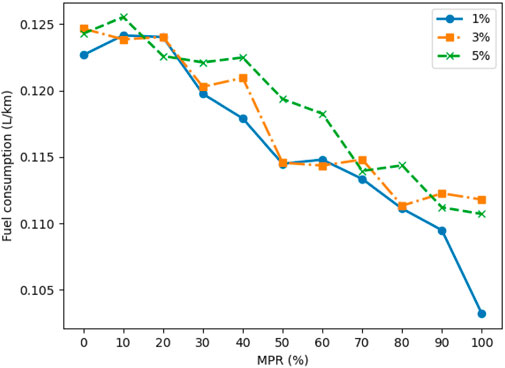
FIGURE 6. Fuel consumption under different MPRs with different proportion of low-speed vehicles.

The correlation between the overall emissions within the road sections and the proportion of low-speed vehicles on the road is a significant concern in addition to the overall energy consumption. Therefore, we conducted a comprehensive investigation of emission indicators of PM, HC, CO₂, and CO across various levels of MPRs for road sections with varying proportions of low-speed vehicles (shown in Figure 7).

FIGURE 7

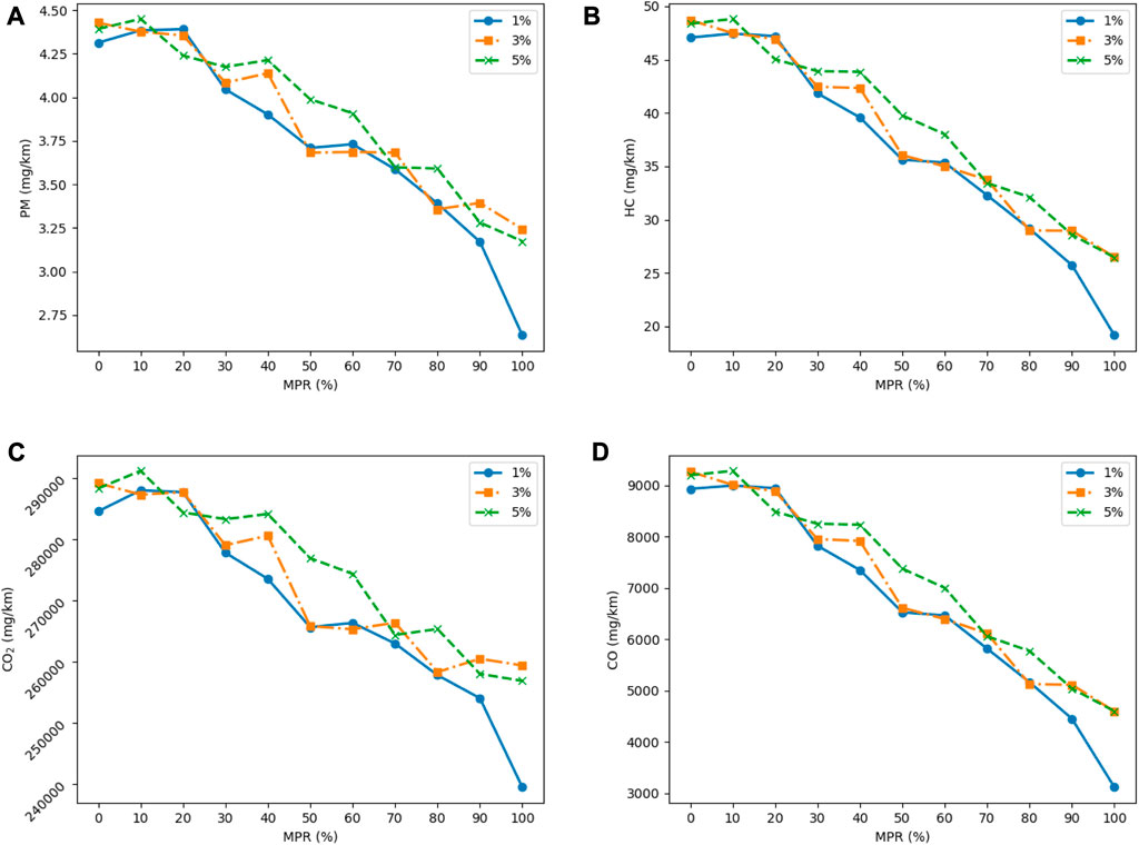
FIGURE 7. Emissions under various MPRs with different proportion of low-speed vehicles. (A) PM emissions. (B) HC emissions. (C) CO₂ emissions. (D) CO emissions.

From the technical perspective, our study investigated the correlation between both fuel consumption and emission of CAVs and shows it is feasible to promote the use of electric CAVs in our daily traffic scenes. Since our experiment results suggest that as MPR increases, there will be a substantial reduction in all four emission indicators as the share of electric CAVs increases. It is also notable that the lowest traffic emissions were observed when low-speed vehicles accounted for only 1% of the share, highlighting the positive impact of autonomous driving systems of CAVs in reducing road emissions. In addition, when autonomous vehicles formed 90%–100% of the traffic flow, emissions were reduced significantly across all four indicators, confirming the environmental friendliness of autonomous systems. Therefore, from the perspective of economics and environmentally friendly policies, we should encourage the wide use of electric CAVs since their green effects on emissions. Meanwhile, we should also introduce a bill to restrict low-speed traffic since our analysis has revealed that the trend of the four emissions is consistent for low-speed vehicle shares of 3%–5%. Moreover, our investigation indicates that at a 3% low-speed vehicle share, CO₂ emissions were 2,400 mg/km lower than at a 5% low-speed vehicle share.

In this section, we have undertaken an analysis of the correlation between the aggregate energy consumption and emissions levels of a given traffic flow and the share of low-speed vehicles present on the road under different MPRs. The experiment results indicate a downward trend in overall energy consumption and emissions as the percentage of CAVs on the roadway increases, specifically in scenarios that involve low-speed vehicles. Furthermore, we have observed a proportionate increase in energy consumption and emissions as the number of low-speed vehicles on the roadway increases, although such patterns may exhibit slight variability over time.

4.2 Electricity consumption

The subsequent analysis is intended to examine the electric consumption of CAVs based on different MPRs, as illustrated in Figure 8. When pure electric vehicles are considered, the data demonstrates that the electricity consumption will rise from 112 Wh/km to 160 Wh/km as the MPR increases from 0% to 100%, in contrast to the previous scenario of completely fuel-driven vehicles. This implies that the overall electricity consumption of the vehicles utilizing the roadway will increase when CAVs take over the road section entirely. The probable explanation is that communication, detection, and collaboration among the vehicles consume more power as the percentage of self-driving vehicles on the road increases (Qu et al., 2022).

FIGURE 8

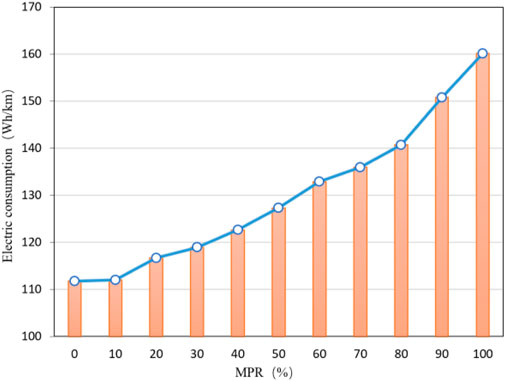
FIGURE 8. Electricity consumption under various MPRs.

4.3 Carbon emissions analysis

Carbon emissions serve as a crucial determinant impacting the ecological environment, with automobile carbon emissions specifically proving to be a crucial target for accomplishing carbon neutrality. As a result, thorough analysis of carbon emissions from varying energy vehicles and the implementation of corresponding optimization measures remains central focuses of the present research. In this section, we present a comparative and analytical exploration of the carbon emissions produced by fuel and electric vehicles different MPR levels, with particular attention to the associated results. Given the heavy reliance of fully electric vehicles on electricity, formula (4) is applied as a uniform unit for analyzing and comparing the CO₂ emissions from these vehicles’ electricity consumed.

$E_{\left({CO}_2\right)}=1\times {10}^3\bullet E_{\left(elec\right)}\bullet \epsilon (4)$

where, $E_{\left({CO}_2\right)}$ is the emission of CO₂, mg/km; $E_{\left(elec\right)}$ is the electricity consumption, Wh/km; $\epsilon$ is the conversion coefficient, it is 0.785 in this paper.

The results of the comparison between carbon emissions of fuel and electric vehicles after conversion are presented in Figure 9. The graph demonstrates that as CAVs increase in the traffic flow, the carbon emissions of fuel vehicles gradually decrease from 28,000 to 24,000 mg/km. However, these indicators still remain at a higher emission level. On the other hand, when the CAVs fully occupy the road section, the carbon emissions of pure electric vehicles increase slightly, yet maintaining an overall lower level at about 110,000 mg/km. This value is 13,000 mg/km lower than the emissions of fuel-driven vehicles when the MPR approaches 100%. These findings highlight the potential of pure electric autonomous vehicles to reduce carbon emissions and promote environmental protection significantly. Therefore, implementing pure electric vehicles with autonomous driving capabilities could be a crucial and feasible approach to reducing carbon emissions.

FIGURE 9

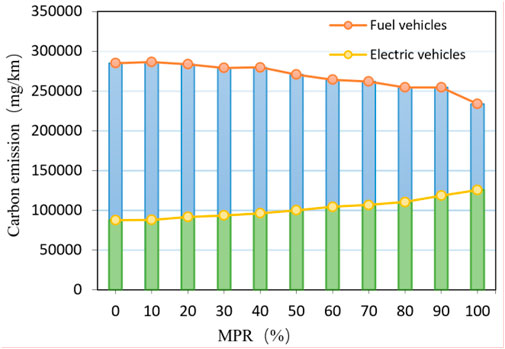
FIGURE 9. Comparison of carbon emissions with electricity conversion.

5 Conclusion

This study examines vehicles’ energy consumption and emissions in autonomous driving intervention traffic extensively on the investigation of energy and electric CAVs. Furthermore, we have also investigated the correlation of fuel, speed, and exhaust emissions on CAVs in the daily urban traffic. The findings demonstrate that as the number of autonomous vehicles on the road increases, the collective energy consumption and emissions of electric and fuel vehicles decrease. Moreover, electric vehicles produce significantly fewer carbon emissions than their fuel counterparts, which serves as a practicable means and a theoretical framework for limiting carbon emissions. Therefore, increasing the percentage of electric vehicles on the roads and transitioning from manual to autonomous driving systems are crucial to curbing carbon emissions.

Data availability statement

The raw data supporting the conclusion of this article will be made available by the authors, without undue reservation.

Author contributions

All authors listed have made a substantial, direct, and intellectual contribution to the work and approved it for publication.

Conflict of interest

The authors declare that the research was conducted in the absence of any commercial or financial relationships that could be construed as a potential conflict of interest.

Publisher’s note

All claims expressed in this article are solely those of the authors and do not necessarily represent those of their affiliated organizations, or those of the publisher, the editors and the reviewers. Any product that may be evaluated in this article, or claim that may be made by its manufacturer, is not guaranteed or endorsed by the publisher.

References

Alvarez, M., Xu, C., Rodriguez, M. A., et al. 2020. Reducing road vehicle fuel consumption by exploiting connectivity and automation: A literature survey. https://arxiv.org/abs/20u11.14805 (accessed on November 30, 2020).

Google Scholar

Barbecho Bautista, P., Urquiza-Aguiar, L. F., and Aguilar Igartua, M. (2021). “Stgt: SUMO-based traffic mobility generation tool for evaluation of vehicular networks,” in Proceedings of the 18th ACM Symposium on Performance Evaluation of Wireless Ad Hoc, Sensor, & Ubiquitous Networks, Alicante, Spain, November 2021, 17–24.

CrossRef Full Text | Google Scholar

Baumgartner, A., Krysiak, F. C., and Kuhlmey, F. (2022). Sufficiency without regret. Ecol. Econ. 200, 107545. doi:10.1016/j.ecolecon.2022.107545

CrossRef Full Text | Google Scholar

Cai, L., Lv, W., Xiao, L., and Xu, Z. (2021). Total carbon emissions minimization in connected and automated vehicle routing problem with speed variables. Expert Syst. Appl. 165, 113910. doi:10.1016/j.eswa.2020.113910

CrossRef Full Text | Google Scholar

China, I. (2018). Energy saving and new energy automotive industry development plan 2012–2020. Available online: https://www.iea.org/policiesandmeasures/pams/china/name-32249-en.php (accessed on August 20, 2018).

Google Scholar

Gov, E. (2018). China—oil and gas export.gov. Available online: https://www.export.gov/article?id=China-Oiland-Gas (accessed on August 20, 2018).

Google Scholar

Huang, J., Song, G., Wu, Y., Zhai, Z., Zhang, Z., and Zhang, L. (2023). A fuel consumption model for mixed traffic flow in multiple connected and autonomous scenarios. IET Intelligent Transport Systems. Wiley, Hoboken, NJ, USA, doi:10.1049/itr2.12340

CrossRef Full Text | Google Scholar

Islam, E. S., Moawad, A., Kim, N., and Rousseau, A. (2019). Vehicle electrification impacts on energy consumption for different connected-autonomous vehicle scenario runs. World Electr. Veh. J. 11 (1), 9. doi:10.3390/wevj11010009

CrossRef Full Text | Google Scholar

Kopelias, P., Demiridi, E., Vogiatzis, K., Skabardonis, A., and Zafiropoulou, V. (2020). Connected & autonomous vehicles–Environmental impacts–A review. Sci. total Environ. 712, 135237. doi:10.1016/j.scitotenv.2019.135237

PubMed Abstract | CrossRef Full Text | Google Scholar

Labanca, N., and Bertoldi, P. (2018). Beyond energy efficiency and individual behaviours: policy insights from social practice theories. Energy Policy 115, 494–502. doi:10.1016/j.enpol.2018.01.027

CrossRef Full Text | Google Scholar

Lamb, W. F., Wiedmann, T., Pongratz, J., Andrew, R., Crippa, M., Olivier, J. G. J., et al. (2021). A review of trends and drivers of greenhouse gas emissions by sector from 1990 to 2018. Environ. Res. Lett. 16 (7), 073005. doi:10.1088/1748-9326/abee4e

CrossRef Full Text | Google Scholar

Li, H., Wang, L., Hu, H., and Bie, Y. (2023). Optimal matching between vehicle speed and lighting at intersection based on traffic risk analysis. ASCE-ASME J. Risk Uncertain. Eng. Syst. Part A Civ. Eng. 9 (2), 04023004. doi:10.1061/ajrua6.rueng-939

CrossRef Full Text | Google Scholar

Lu, Q., Chai, J., Wang, S., Zhang, Z. G., and Sun, X. C. (2020). Potential energy conservation and CO₂ emissions reduction related to China’s road transportation. J. Clean. Prod. 245, 118892. doi:10.1016/j.jclepro.2019.118892

CrossRef Full Text | Google Scholar

Ma, J., Hu, J., Leslie, E., Zhou, F., Huang, P., and Bared, J. (2019). An eco-drive experiment on rolling terrains for fuel consumption optimization with connected automated vehicles. Transp. Res. Part C Emerg. Technol. 100, 125–141. doi:10.1016/j.trc.2019.01.010

CrossRef Full Text | Google Scholar

McConky, K., and Rungta, V. (2019). Don’t pass the automated vehicles!: system level impacts of multi-vehicle CAV control strategies. Transp. Res. Part C Emerg. Technol. 100, 289–305. doi:10.1016/j.trc.2019.01.024

CrossRef Full Text | Google Scholar

Oswald, D., Scora, G., Williams, N., et al. (2019). “Evaluating the environmental impacts of connected and automated vehicles: potential shortcomings of a binned-based emissions model,” in 2019 IEEE intelligent transportation systems conference (ITSC), Auckland, New Zealand, October 2019, 3639–3644.

CrossRef Full Text | Google Scholar

Paul Anthikkat, A., Page, A., and Barker, R. (2013). Risk factors associated with injury and mortality from paediatric low speed vehicle incidents: A systematic review. Int. J. Pediatr. 2013, 1–17. doi:10.1155/2013/841360

CrossRef Full Text | Google Scholar

Pribyl, O., Blokpoel, R., and Matowicki, M. (2020). Addressing EU climate targets: reducing CO2 emissions using cooperative and automated vehicles. Transp. Res. Part D Transp. Environ. 86, 102437. doi:10.1016/j.trd.2020.102437

CrossRef Full Text | Google Scholar

Qin, Y., Wang, H., and Ran, B. (2018). Stability analysis of connected and automated vehicles to reduce fuel consumption and emissions. J. Transp. Eng. Part A Syst. 144 (11), 04018068. doi:10.1061/jtepbs.0000196

CrossRef Full Text | Google Scholar

Qu, X., Zhong, L., Zeng, Z., Tu, H., and Li, X. (2022). Automation and connectivity of electric vehicles: energy boon or bane? Cell Rep. Phys. Sci. 3 (8), 101002. doi:10.1016/j.xcrp.2022.101002

CrossRef Full Text | Google Scholar

Rios-Torres, J., and Malikopoulos, A. A. (2018). Impact of partial penetrations of connected and automated vehicles on fuel consumption and traffic flow. IEEE Trans. Intelligent Veh. 3 (4), 453–462. doi:10.1109/tiv.2018.2873899

CrossRef Full Text | Google Scholar

Romero, J. P., and Gramkow, C. (2021). Economic complexity and greenhouse gas emissions. World Dev. 139, 105317. doi:10.1016/j.worlddev.2020.105317

CrossRef Full Text | Google Scholar

Song, G., and Yu, L. (2011). Characteristics of low-speed vehicle-specific power distributions on urban restricted-access roadways in beijing. Transp. Res. Rec. 2233 (1), 90–98. doi:10.3141/2233-11

CrossRef Full Text | Google Scholar

Tu, R., Alfaseeh, L., Djavadian, S., Farooq, B., and Hatzopoulou, M. (2019). Quantifying the impacts of dynamic control in connected and automated vehicles on greenhouse gas emissions and urban NO2 concentrations. Transp. Res. Part D Transp. Environ. 73, 142–151. doi:10.1016/j.trd.2019.06.008

CrossRef Full Text | Google Scholar

Wang, L., Li, H., Li, S., and Bie, Y. (2022). Gradient illumination scheme design at the highway intersection entrance considering driver’s light adaption. Traffic Inj. Prev. 23 (5), 266–270. doi:10.1080/15389588.2022.2055004

PubMed Abstract | CrossRef Full Text | Google Scholar

Woodman, R., Lu, K., Higgins, M. D., et al. (2019). “A human factors approach to defining requirements for low-speed autonomous vehicles to enable intelligent platooning,” in 2019 IEEE Intelligent Vehicles Symposium (IV), Paris, France, June 2019, 2371–2376.

CrossRef Full Text | Google Scholar

Xiong, S., Ji, J., and Ma, X. (2019). Comparative life cycle energy and GHG emission analysis for BEVs and PHEVs: A case study in China. Energies 12 (5), 834. doi:10.3390/en12050834

CrossRef Full Text | Google Scholar

Yao, Z., Wang, Y., Liu, B., Zhao, B., and Jiang, Y. (2021). Fuel consumption and transportation emissions evaluation of mixed traffic flow with connected automated vehicles and human-driven vehicles on expressway. Energy 230, 120766. doi:10.1016/j.energy.2021.120766

CrossRef Full Text | Google Scholar

Ye, L., and Yamamoto, T. (2019). Evaluating the impact of connected and autonomous vehicles on traffic safety. Phys. A Stat. Mech. its Appl. 526, 121009. doi:10.1016/j.physa.2019.04.245

CrossRef Full Text | Google Scholar

Zhao, B., Lin, Y., Hao, H., and Yao, Z. (2022). Fuel consumption and traffic emissions evaluation of mixed traffic flow with connected automated vehicles at multiple traffic scenarios. J. Adv. Transp. 2022, 1–14. doi:10.1155/2022/6345404

CrossRef Full Text | Google Scholar

Zong, S. (2019). How connected autonomous vehicles would affect our world? a literature review on the impacts of CAV on road capacity, environment and public attitude. MATEC Web Conf. EDP Sci. 296, 01007. doi:10.1051/matecconf/201929601007

CrossRef Full Text | Google Scholar