Modelling and optimizing microgrid systems with the utilization of real-time residential data: a case study for Palapye, Botswana

1 Introduction

Solar energy has steadily gained acceptance as a viable resource for small to medium-scale energy systems for residential users. The increasing affordability of solar PV systems has made renewable energy resources more appealing for integration in microgrid systems (Qazi, 2017). The Levelized Cost of Electricity (LCOE) for residential solar PV systems is estimated to be down to 0.05 USD/kWh by 2030 (sley, 2021). Residential households will play a crucial role in the next-generation of electricity systems in Africa (IRENA, 2022). Establishing solar microgrid systems can benefit the shared use of solar energy among community residential consumers. Solar microgrids have become increasingly popular due to the widespread availability of solar energy resources (Tajjour and Singh Chandel, 2023). A microgrid is a bounded section of the electricity transmission and distribution network that combines locally distributed generation sources, energy storage devices, and regulated electrical loads to produce a self-sufficient energy system (Cagnano et al., 2020).

Botswana receives a significant amount of solar insolation daily, with a maximum of 6.2 kWh/m²/day in the Kgalagadi and Ghanzi districts and a minimum of 5.5 kWh/m²/day in the country’s east central and south north-eastern regions (Dabla, 2021). The government has created several incentive programs to promote the use of solar energy. These include adoption of solar rooftops and home systems. The government established an isolated solar microgrid system of 5.7 kW capacity with battery storage in the village of Motshegaletau to power a school, clinic, some residential houses, and a business centre (Situmbeko, 2018). A hybrid PV-wind system was evaluated and designed to provide electricity for the rural areas of Jamataka village in Botswana’s north-eastern region (Ravi et al., 2022). The survey was conducted to determine the power consumption of the households in the village. The financial analysis using the Net Present Cost (NPC) method revealed that the PV/wind/battery system configuration delivers the greatest economic energy advantages to the community of Jamataka. The electricity usage is 165.29 kWh/day, the peak and primary load demand is 27.31 kW, and the total load is 1165.58 kWh/day. The developed system can help the community reduce the use of firewood, and lower desert encroachment and reduction in the generation of smoke with an overall environmental protection. Further, the system can enhance economic development in the community.

Because solar power is diurnal, a backup power source is required to ensure that residential consumers have uninterrupted electricity supply. Control and EMS are crucial in maintaining a microgrid system’s continuous power supply to loads. The key nature of an EMS is to regulate the power within the components of the microgrid system (Hasan and Bin Arif, 2018). Hierarchical and droop control are two common control systems for microgrids. Model Predictive Control (MPC), which employs machine learning techniques, is a fast-growing technology for power management in a microgrid system (Hu et al., 2020). Through control strategies and load mixing, consumers can make savings on their electricity bills (Palaniappan et al., 2017). Residential energy demand modelling is necessary to identify temporal energy consumption patterns.

Demand-side energy management in residential households relies heavily on energy forecasting. Smart meters are essential to studying energy usage traits in a residential building. Electricity usage patterns at the individual household level are dependent on multiple factors such as building design, lifestyle, occupancy behaviour, and appliance ownership and use (Zhang et al., 2019). Mohammad Amir et al. (Mahlooji et al., 2013) developed a battery system to reduce the peak demand of the electricity with the reduced losses. The high variability of daily energy usage makes it very complex to accurately model and simulate the energy consumption data of residential households (Alvarez et al., 2018). Residential energy demand modelling is necessary to identify energy consumption patterns. Analysis of energy consumption data can be classified as predictive analytics, prescriptive analytics, and descriptive analytics. Descriptive analytics reveals the structure and nature of the data set, while predictive analytics forecasts the nature of the data in the future through historical data. The descriptive analytics comprises the measurement of central tendency and dispersion. The predictive analysis includes techniques such as forecasting, regression, and clustering (Deb et al., 2017a). Time series research identifies daily energy patterns that reveal energy forecasting coefficients. Prescriptive analytics blends descriptive and predictive analysis to make suggestions based on data projections (Leonori et al., 2016).

Obaro et al. (2023) performed a study on the modelling and energy management of an off-grid distributed energy system for a typical village in South Africa using a MATLAB program through an enhanced mixed integer nonlinear programming optimization algorithm. The study aimed to design a reliable energy system while considering a scenario with a combined load demand of sixty households. The system’s results showed reliable system improvement and a model for an ideal distributed energy system that is also cost-effective and environmentally friendly. A hybrid distributed energy system of solar, wind, and biomass energy was designed, modelled, and optimized using the HOMER program for a remote area in western China encompassing residential, small-scale industrial, commercial, and agricultural power loads. The study showed that the system is feasible, economical, and environmentally friendly.

Distributed energy systems powered by renewable energy are key to lowering carbon emissions. When planning, modelling, and optimizing distributed energy systems, evaluating various models, or combining models is essential to produce more reliable outcomes. Srivastava et al. (2022) proposed a solar PV for the urban cities without requiring any additional land. Various energy plans, policies and government initiatives were reviewed to access and analyze Southern African countries’ electricity challenges and carbon emissions Justo Jackson et al. (2013). The results suggest that off-grid alternatives to fossil fuels should be considered to improve electricity access and eradicate energy poverty in this region, which has a wealth of renewable energy resources, including hydro, solar, wind, biomass, and geothermal energy (Justo Jackson et al. (2013)).

Battery Energy Storage System (BESS) reduces power supply variability between electrical loads and generation units (Abdi et al., 2017; Alzahrani et al., 2017; DW, 2015). BESS is vital for urban microgrid systems to provide power to loads during the island mode. A BESS is required for urban microgrid systems to provide electricity to loads during the island mode. It communicates with the DC/DC converter, DC/AC inverter, DC link capacitor, and the community solar PV microgrid system (Farrokhabadi et al., 2018). The buck-boost converter as a DC/DC converter topology enables the charge and discharge of the BESS (Farrokhabadi et al., 2018; Kondrath, 2018). Energy Storage Systems (ESS) configurations exist in two states, namely, distributed and aggregated ESS. When compared to distributed ESS, aggregated ESS is better suitable for microgrids because it efficiently suppresses power fluctuation in the microgrid system (DW, 2015; Li and Joós, 2007). The BESS manages energy in the microgrid system by performing load levelling and peak load shifting. Local voltage support, grid contingency assistance, and load shifting are ancillary services that the ESS provides to the microgrid system (Farrokhabadi et al., 2018). The BESS models utilize the commonly established electrochemical batteries or regulated voltage sources (Olivier TremblayLouis and DessaintLouis, 2007). BESS models can respond to the control system instructions and activate the reserve in approximately 20 milliseconds. BESS capacity and lifetime are affected by variables such as Depth of Discharge (DOD), rate of discharge, and temperature. Eq. 1 illustrates the capacity of a battery expression (Alzahrani et al., 2017):

$B_{capacity}=\frac{E_{load}\ast D_{off}}{{DOD}_{\mathit{max}}\ast n_{temp}}(1)$

$E_{load}$ is the load supplied to the microgrid system during periods of low electrical power supply by the DG unit in ampere-hours, $D_{off}$ is the number of days the microgrid is operating in island mode, ${DOD}_{\mathit{max}}$ is the depth of discharge at maximum level and $n_{temp}$ represents the temperature correction factor. Lithium-ion batteries are the most commonly used battery type for community solar PV microgrids because of their unique characteristics, including high energy density, low weight, and long-life duration (Kularatna, 2015).

Since the reliability of energy delivery to consumers is affected by the stability of the utility system. Electricity supply unreliability will primarily affect residential consumers in urban areas. Due to many electrical appliances and structures in use every day of the year, metropolitan areas have high electricity consumption. According to the World Energy Balances 2019, residential power usage climbed from 42 kilo tonnes of oil equivalent (KToe) in 2004 to 88 KToe in 2017 (U. E. I. Administration, 2019). Energy provision from solar photovoltaics presents an innovative method to alleviate the electricity need mainly among people living in residential areas. An assessment on the rooftop solar PV system (microgrid) design for an urban settlement will be conducted whereby people will be sharing electrical loads through the system. The system to be designed will be grid tied. The research begins with the measurement of the electricity load in an exemplary building over a period. Afterward, a solar PV system will be designed and simulated for a single household. After that, a solar PV microgrid system will be modelled and simulated for the urban residential quarter (25 residential houses with similar load profiles). The control and energy management approach used will assure optimal energy generation by the solar PV system, resulting in lower monthly electricity expenditures. An overview will be undertaken to emphasize the need for microgrid systems through a brief economic assessment.

2 Methodology for system model

This section of the paper comprises the design and sizing of the solar PV microgrid system for a community of residential households. Figure 1 shows the framework of the solar microgrid system.

FIGURE 1

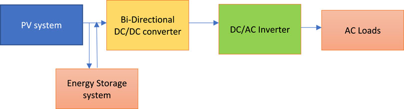
FIGURE 1. The framework of the solar microgrid system.

The solar PV microgrid system includes five major components, namely, the Solar PV system, Energy Storage System (ESS), bi-directional DC/DC converter, DC/Alternating Current (AC) inverter, and AC electrical loads. Subsections 2.1 and 2.2 illustrate the sizing and modelling of the parameters for the model.

2.1 Load metering

The primary goal of load metering was to determine the capacity of the community solar PV microgrid system for the residential community in Palapye, Botswana. The principal residence where the studies were conducted provided the fundamental energy use patterns typical of urban residential settings. The measurement period was for 12 months to have a yearly overview of energy consumption in a residential household. A smart metering device was installed to monitor electrical parameters such as voltage, current, and power factor. Time series and regression analysis are two smart meter data analytics used in the study. Figure 2A shows physical connection of energy measuring devices to the distribution board. Figure 2B depicts the daily electricity usage and the peak power recorded in the building.

FIGURE 2

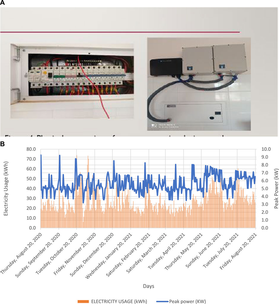
FIGURE 2. (A) Physical connection of energy measuring devices to the distribution board. (B) Daily electricity usage and the peak power recorded.

From Figure 2B, the maximum daily peak power recorded was 9.2419 kW. Since all the residential houses in the community were similar and contained the similar electrical appliances, it was assumed that each resident’s daily peak usage would be 10 kW peak. The 10 kW for 25 residential families in the community corresponds to a planned central solar PV power system of 250 kW. The irregularity of daily energy usage makes it very complex to accurately model and simulate the energy consumption data of residential households. The load metering analysis of the residential household is necessary to identify energy usage patterns to optimize the efficiency of the EMS in the microgrid system.

2.1.1 Regression analysis

The regression analysis reveals the best-case load model to represent the typical load profile of a residential household. Load forecasting is classified into three types: short-term, medium-term, and long-term forecasting (Singh and Yassine, 2018). Short-term load forecasting was chosen for residential load profile because it has a greater prediction accuracy than medium and long-term types (Aurangzeb, 2019; Ridwana et al., 2020). The most commonly used regression analysis is simple linear regression (LR), which is defined by a random variable (y) that can be described as a linear function of another random variable (x) (Nelson and Biswas, 2015). The relationship between the variables is expressed in Eq. 2:

$y={\beta }_o+{\beta }_{1}x+\epsilon (2)$

where y is the response variable, x is the predictor variable, ${\beta }_o$ and ${\beta }_1$ are regression coefficients, and $\epsilon$ is an error that accounts for the discrepancy between the predicted and observed data. Using the smart metering data, a linear model is generated for electricity usage in the household. A coefficient of determination (R²) is used to assess the efficacy of the linear model (Nelson and Biswas, 2015). The coefficient of determination is expressed in Eq. 3

$R^2=1-\frac{{\displaystyle \sum }{\left(y_i-\widehat{y_i}\right)}^2}{{\displaystyle \sum }{\left(y_i-\widehat{y_i}\right)}^2}(3)$

where ${\left(y_i-\widehat{y_i}\right)}^2$ represents the sum of the squared errors and ${\left(y_i-\overline{y_i}\right)}^2$ represents the total sum of squares. R² is a number between 0 and 1. The closer R² is to 1, the more the model accurately indicates that the predictor variables account for a large portion of the variability in response variables. Another way to validate a prediction model’s performance is through the Root Mean Square Error (RMSE) expressed in Eq. 4 (Zhang et al., 2018).

$RMSE=\sqrt{\frac{{\displaystyle \sum _{i=1}^N}{\left(y_i-{\widehat{y}}_i\right)}^2}{N}}(4)$

where $y_i$ denotes the actual electricity consumption of the household j, $\widehat{y_i}$ denotes the predicted electricity consumption, and N is the number of observations.

2.1.2 Time series

Time series analysis uses a model to predict future values based on previously observed values (Chou and Duc Son, 2018). Notable machine learning algorithms for time series forecasting include Artificial Neural Networks (ANN), Support Vector Machine (SVM), and Autoregressive Integrated Moving Average (ARIMA). The ARIMA algorithm is a linear equation in which the predictors are the dependent variables lags and the prediction error (Kuster et al., 2017). The ARIMA model can be mathematically expressed in Eq. 5.

$Y_t=c+\varnothing Y_{t-1}+\varnothing Y_{t-2}\dots +{ϵ}_t(5)$

where $Y_t$ represents the dependent variable, subscript $t$ is an integer index, $c$ is a constant, $\varnothing$ represents the magnitude of the autocorrelation and ${ϵ}_t$ represents the error.

The ARIMA model forecasts a time series based on its historical values. A form of ARIMA, SARIMA, uses a seasonal pattern in linear forecasting (Chou and Duc Son, 2018). The SARIMA method can be expressed mathematically in Eq. 6.

$Y_t=c+\varnothing Y_{t-s}+{ϵ}_t(6)$

where subscript $s$ represents the number of lags comprising one full seasonality period. The SARIMA model comprises a linear combination of seasonal past values and forecast errors (Deb et al., 2017b). The Support Vector Machine (SVM) is another time series method consisting of a hybrid of the Support Vector Regression (SVR) and the SVM, which uses element boundary variables to address function fitting problems (Zhang et al., 2019).

2.2 Microgrid system model design

The community solar PV microgrid system design will be conducted on the MATLAB program, namely, Simulink/Simscape, by gathering components from the library block of Sim-power frameworks. The microgrid system exists in two primary states, namely, island and grid-connected mode of operation. The residential households’ maximum load demand will be approximated as 250 kW. The simulation conducted in MATLAB is for a single day; the peak-daily profiles from the residential household in the experiment were utilized as daily load profiles for 25 residential homes in a community. The three-phase load block from the Simscape library was utilized, and the model structure type selected has constant impedance.

2.2.1 Solar PV system modeling

The generic mathematical model of an ideal PV cell is expressed in Eq. 7:

$I=I_{PV}-I_O\left[\mathit{exp}\left(\frac{\left(N_{S}kT\right)V+R_{s}I}{q\alpha }\right)-1\right]-\frac{V+R_{s}I}{R_{sh}}(7)$

The current created by incoming light is represented by ${\mathrm{I}}_{\text{PV}}$, the diode saturation current is represented by ${\mathrm{I}}_{\mathrm{o}}$ and the series and equivalent shunt resistances of the array are depicted by ${\mathrm{R}}_{\mathrm{s}}\text{and}{\mathrm{R}}_{\text{sh}}$. The ideality factor $\left(\mathrm{\alpha }\right)$, is a constant that depends on the PV cell technology used by the manufacturer (Bellia et al., 2014). Other parameters include ${\mathrm{N}}_{\mathrm{s}}$ which is the number of cells in series, $\mathrm{k}$ is the Boltzmann’s constant (1.3806503 * 10⁻²³ J/K), T (K) is the diode temperature, and $\mathrm{q}$ represents the charge of an electron (1.60217646 * 10⁻¹⁹ C) (Singh et al., 2016).

Table 1 provides the module parameters for the PV panel (Solar Tech Energy ASC-6P-72-300). In summary, the 250 kWp planned solar microgrid system requires 15 solar modules, 4 Strings and 13 arrays with a string voltage of 546.75 V.

TABLE 1

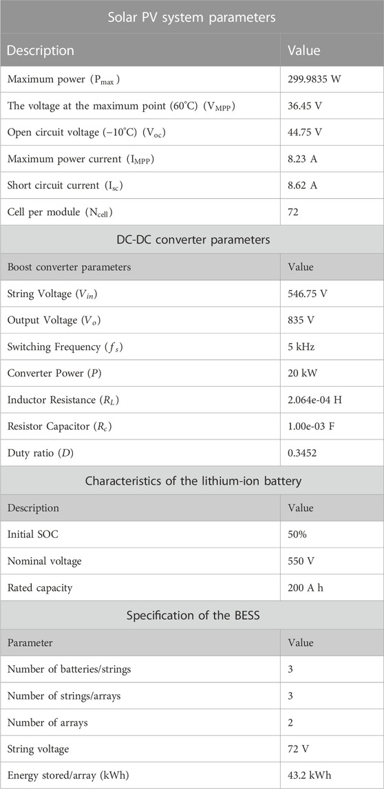
TABLE 1. System design parameters.

2.2.2 DC-DC boost converter

The Distributed Generation (DG) unit of the community microgrid system is an erratic source that generates a highly variable output voltage. Therefore, depending on the loads’ energy requirements, a DC/DC converter is needed to lower voltage ripples and serve as either a step-up or step-down voltage device. The boost converter specs are listed in Table 1.

The converter connects the solar PV system to the DC microgrid system Zammit et al. (2018). In addition, the boost converter may serve as a voltage booster for the DC bus (Farrokhabadi et al., 2018). Inductors, capacitors, and Metal Oxide Semiconductor Field Effect Transistor (MOSFET) devices with switching functions make up the converter, which controls the voltage flow according to the energy needs. Finally, the energy storage components are charged and discharged using the bi-directional converter (Lee et al., 2011).

2.2.3 Battery energy storage system (BESS) modelling

The battery helps to balance electricity in a microgrid by acting as a load or generator during the charging and discharging phases. Lithium-Ion batteries are widely utilized in solar community microgrids as they display higher Depth of Discharge (DoD) than other battery types such as lead-acid and nickel-hydride batteries (Bila et al., 2016; Farrokhabadi et al., 2018; Vetter and Rohr, 2014). Eq. 8 illustrates the capacity of a battery.

$B_{capacity}=\frac{E_{load}\ast D_{off}}{{DOD}_{\mathit{max}}\ast n_{temp}}(8)$

where $E_{load}$ represents the load supplied to the microgrid system during periods of low electrical power supply by the DG unit in ampere-hours, $D_{off}$ is the number of days the microgrid is operating in island mode, ${DOD}_{\mathit{max}}$ is the depth of discharge at maximum level and $n_{temp}$ represents the temperature correction factor. Factors such as DoD, State of Charge (SOC), and temperature affect capacity and life (Alvarez et al., 2018).

A buck-boost converter topology was utilized to discharge and charge the battery in the microgrid system. The BESS comprises a lithium-ion battery model, and a MOSFET-driven circuit to enable the charging and discharge of the battery depending on the available power in the DC bus of the microgrid system. A voltage reference of 835 V is set as the DC bus voltage. It also includes a control scheme that utilizes PID controllers and Pulse Width Modulation (PWM) DC-DC generators to boost the converter’s output and the desired load voltage level in the microgrid system. PID control is widely used in automation and engineering to govern a wide range of operations, such as power management, using a control loop feedback mechanism (Shezan et al., 2023). Adaptive neuro fuzzy control system proposed by (Bramareswara Rao et al., 2022) shows the good power quality indices. Table 1 presents the characteristics of the lithium-ion battery.

The battery was rated as 550 V due to the $V_{mpp}$ of the solar PV module that is rated as 546 V; thereby, during periods of low solar radiation, the battery capacity will be able to meet the desired DC bus voltage of 835 V. The aggregate configuration for the battery packs will be utilized, whereby all the lithium-ion battery units will be stored in a central location (DW, 2015). The system design calculations dictate that approximately 40% of the daily energy usage is at night; thus, estimates for a 100-kWh battery system were designed. Table 1 provides the battery array specifications.

2.2.4 Grid-connected inverter control

The microgrid and its link to the utility grid defines the grid-connected mode of operation. An analogue circuit built of a two-level converter consisting of switching devices changes the waveform of DC voltage to AC voltage is used in a grid-connected inverter. A grid-connected inverter synchronizes the microgrid’s frequency and voltage with the utility grid (Rahimi et al., 2018). The converter is connected to an inductor-capacitor-inductor filter, removing harmonics in the output waveforms and yielding a pure sine wave.

2.2.4.1 Inner control loop

A Voltage Source Inverter (VSI) control system between the inverter and the grid is necessary to synchronize the frequency and allow the desired currents to inject the desired levels of active (P) and reactive power (Q) for certain measured grid voltages (Kabiri et al., 2013) Figure 3 depicts the control scheme of a three-phase grid-connected inverter.

FIGURE 3

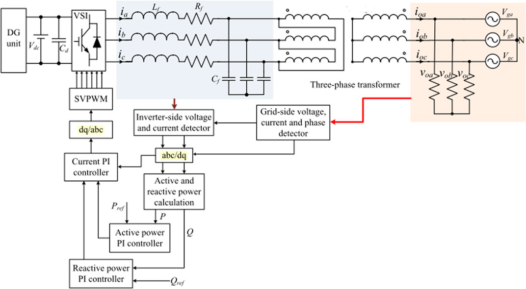
FIGURE 3. The control scheme of a three-phase grid-connected inverter in a microgrid. SOURCE (Chen et al., 2018).

Eq. 9 expresses the grid-connected inverter’s mathematical control model:

$\left[\begin{array}{c}{u}_d\\ u_q\end{array}\right]=L\frac{d}{dt}\left[\begin{array}{c}{i}_d\\ i_q\end{array}\right]+R\left[\begin{array}{c}{i}_d\\ i_q\end{array}\right]+\omega L\left[\begin{array}{c}{-i}_q\\ i_d\end{array}\right]+\left[\begin{array}{c}{e}_d\\ e_q\end{array}\right](9)$

where the grid voltage park conversion component is represented by $e_d$ and $e_q$, and the elements of the park transformation of the inverter output are represented by ${\mathrm{u}}_{\mathrm{d}}$ and $u_q$. The active and reactive transformation components of the inverter current are represented by $i_d$ and $i_q$ respectively. $\omega$ and $L$ represent the angular grid frequency and inductance between the grid-connected inverter and grid, respectively. A closed-loop current regulatory powers a high-frequency PWM switching controller. The Direct-Quadrature (DQ) transformation control is employed because it can run near a power factor of unity with any amount of solar energy.

As indicated in Figure 3, P and Q can be processed from the generator to the load with bidirectional control and vice versa. PID and Phase Locked Loop (PLL) controllers are included in the DQ control, and they can regulate DC variables and extract the grid voltage’s phase angle, respectively (Phuong et al., 2015). The major function of the inverter side control is to extract as much electricity as possible from the solar PV system and convert it to AC power. The active and reactive inverter currents can be removed using the DQ transformation. PID controllers are then used to compensate for current error between the measured output current and the appropriate injected current into the utility grid. Grid-side control includes regulating the amount of power fed into the grid and grid synchronization. PWM techniques regulate the active and reactive components of current delivered to the grid through a current control loop (Ahmed and Abdelhalim, 2012). Inverter specifications are listed in Table 2.

TABLE 2

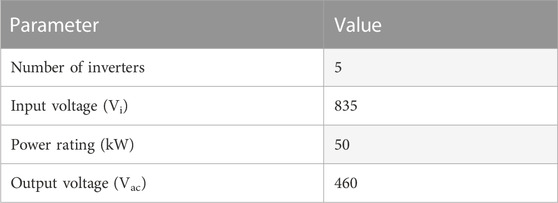
TABLE 2. Inverter specifications.

2.2.4.2 LCL filter design

The LCL filters are extensively used to connect inverters to the grid because they serve the primary objective of reducing harmonics in the output, presenting a resonant frequency, and giving superior fading of the ripple currents in the grid current (Ngoc Nam et al., 2019). The maximum allowed Total Harmonic Distortion (THD) from the grid side current should be within 5% according to the IEEE-519 standard (Hasiah et al., 2014). The distortion of voltage or current by harmonics is known as THD. Table 3 provides the parameters for the filter design.

TABLE 3

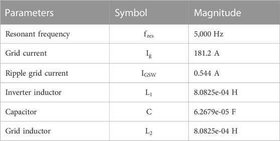
TABLE 3. Filter design parameters.

2.3 Optimization through fuzzy logic control (FLC)

The FLC control system is an alternative technique for energy management in microgrids instead of PID controllers. Through guiding principles, the FLC system may efficiently regulate the power flow between the microgrid system’s components (Al-Sakkaf et al., 2019).

2.3.1 Energy flow in microgrid system through fuzzy logic control

The FLC executes power management in the microgrid system per the energy requirements. Maintaining the desired DC bus voltage required for the constant power supply to the electrical loads in a settlement is the fundamental goal of the control system. The FLC algorithm-maintained power between the PV unit, battery, and utility grid. The FLC structure comprises input and output variables. Figure 4 illustrates the FLC structure.

FIGURE 4

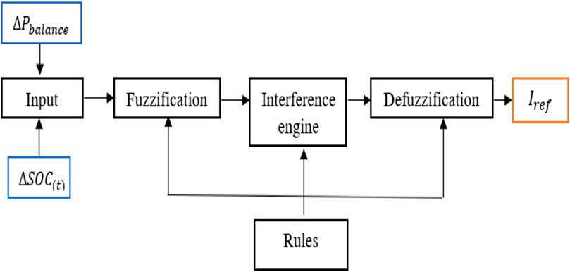
FIGURE 4. FLC operation structure.

The change in power and the variation in battery SOC will serve as the fuzzy logic’s input variables, and the output will be a current reference (Iref). The fuzzification process involves the transformation of a crisp quantity into a fuzzy quantity (Reyes-García and Torres-Garcia, 2022). The interference engine is guided by a set of rules based on “IF” statements between the two inputs, $∆P_{balance}\text{and}∆SO{C}_{\left(t\right)}$. The defuzzification process involves converting linguistic values into crips values. The generated current reference instructs the grid-connected inverter when to discharge electricity from the grid and when to recharge the grid with extra solar PV power generated. The primary purpose of the FLC is to maintain the desired DC bus voltage of 835 V required by the loads. The current reference generated by the FLC sends a control signal to the components of the microgrid, such as a solar PV system, a battery, or the electric grid to discharge or charge power in the microgrid bus to achieve the desired bus voltage. The desired input range is the data range of the battery’s SOC. Eqs 10 and 11 represent the mathematical expressions for the input battery SOC.

${SOC}_{\mathit{min}}\le {SOC}_{\left(t\right)}\le {SOC}_{\mathit{max}}(10)$

$∆SO{C}_{\left(t\right)}={SOC}_{original\left(t\right)}-{SOC}_{now\left(t\right)}(11)$

where ${SOC}_{\mathit{min}}$ and ${SOC}_{\mathit{max}}$ reflect the battery’s minimum and maximum SOC. The charging and discharging of the battery are time dependent. When solar PV generation is negligible at night, the battery will supply the DC microgrid with the desired voltage. The difference between the original SOC and the actual SOC of the battery is computed to determine the change in $∆SO{C}_{\left(t\right)}$. Another input for the FLC algorithm was the power balance ($\left.∆P_{balance}\right)$ in the microgrid system. Eq. 12 represents the power balance.

$∆P_{balance}=P_{pv}-P_{load}(12)$

where $P_{load}$ and $P_{pv}$ depict the load demand power and the solar PV generated power, respectively. Excess solar PV power charges the battery when the P balance is positive. Once the battery is fully charged, the excess electricity generated by the solar PV system is fed into the grid.

3 Results analysis

The solar microgrid system’s data analysis and performance assessment were conducted in simulation environments such as SPSS and MATLAB/Simulink.

3.1 Load metering analysis

Smart meter data analytics were used in the load metering analysis. The regression and time series analyses were carried out using simulation software.

3.1.1 Overall load profiles

Using statistical data from August 2020 and August 2021, the average daily electricity usage (kWh) of the house in experimentation is 27.39991 kWh. Graphs for the 15-min intervals, hourly and daily intervals are illustrated below. Figure 5 provides a graphical representation of the 15-min interval energies record for the 21st of August 2020.

FIGURE 5

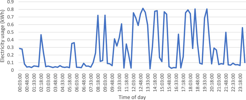
FIGURE 5. The 15-min energies.

From Figure 5, the peak energy demand occurs around 2,300 h. The peaks and valleys across the results are usually due to the behavioural usage behaviour of the residents. Therefore, the peak energy demand varies daily and depends on the inhabitants’ energy usage behaviour in the residential household. Figure 6 provides a weekly load profile for the house in experimentation.

FIGURE 6

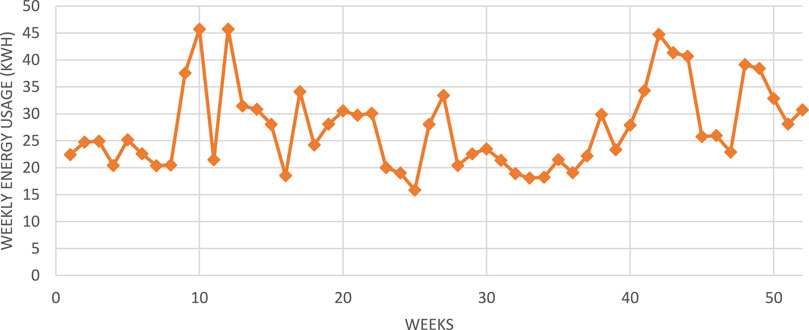
FIGURE 6. Weekly energy consumption load profile (kWh).

The average weekly analysis reveals an average electricity usage of 27.28 kWh. Between week eight and week 13, as illustrated by Figure, a steep rise was identified, indicating the increased Air Conditioner (AC) usage in the residential household. Another steep climb occurred between weeks 40 and 45. The maximum and minimum weekly energy usage was recorded at 45.7 kWh and 15.84 kWh. Figures 7, 8 represent the daily electricity usage and peak power, respectively, for the residential household in experimentation.

FIGURE 7

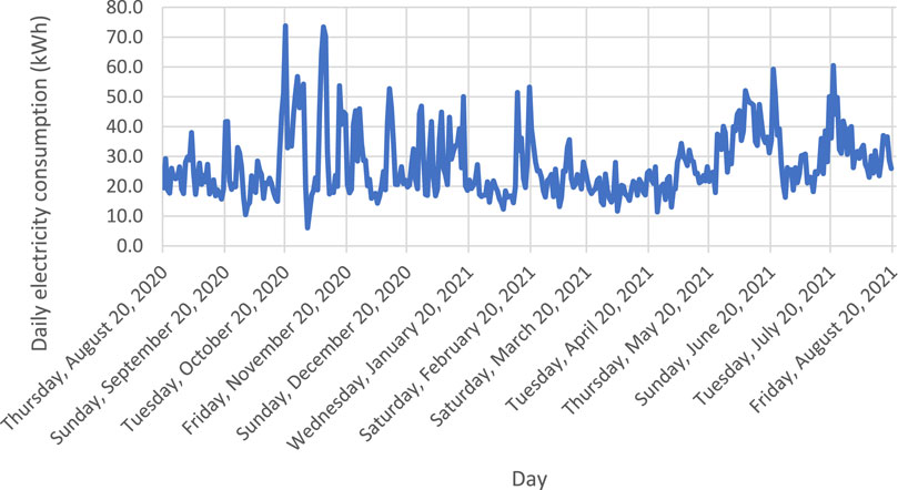
FIGURE 7. Daily electricity usage Profile (kWh).

FIGURE 8

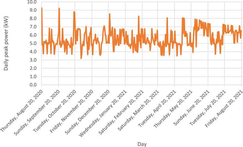
FIGURE 8. Daily peak power.

From Figures 7, 8, it can be concluded that high peaks are experienced during the week, and low peaks occur during the weekends. The daily average electricity usage was 27.4 kWh from the experimental recordings, while the daily peak power usage was recorded at 5.575 kW. The maximum daily electricity usage and peak power was recorded at 73.797 kWh and 9.249 kW, respectively.

3.1.2 Seasonal analysis

The yearly metered data was sampled through the year’s summer, autumn, spring, and winter. The y-axis is the electricity consumption in kW and the x-axis is the days/months of the respective seasons. In addition, daily usage graphs of peak days of the seasons experienced in Botswana were prepared. A semi-arid climate throughout the year characterizes Botswana’s weather; thus, it generally experiences summer and winter seasons. The summer period is from November to March and the winter period is from May to August. Figure 9 and Figure 10 depict the peak load profiles for summer and winter period, respectively.

FIGURE 9

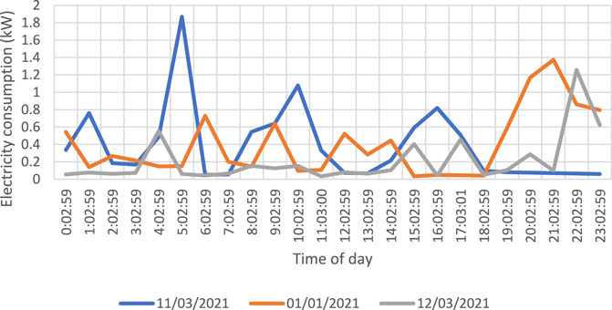
FIGURE 9. Peak hourly profiles during the summer period.

FIGURE 10

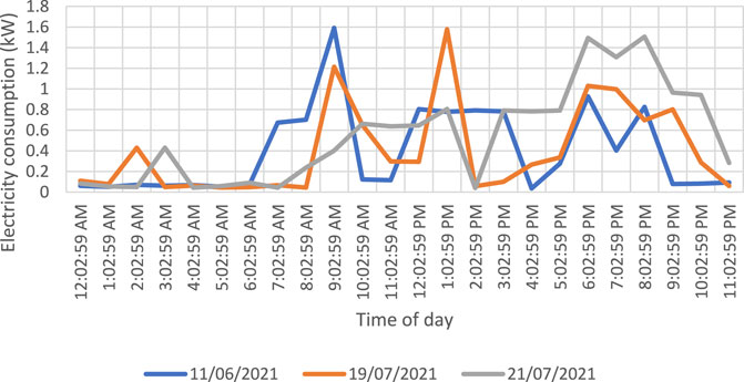
FIGURE 10. Peak hourly profiles during the winter season.

The highest hourly peak electricity usage was recorded during the summer season, followed by the season winter. From Figure 9, the peak hourly usages are in the early mornings and late evenings. The winter season from Figure 10 indicates that the energy peaks occur late morning, early afternoon, and evening. Figure 11 provides a graphic description of the seasonal electricity usage by month in Botswana.

FIGURE 11

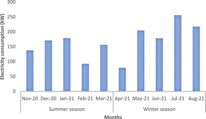
FIGURE 11. Seasonal electricity usage by months.

The dataset was analysed, and it revealed the following:

The mean electricity consumption was recorded at 0.229563 kW in the summer season, with the maximum and minimum hourly usage at 1.87773 kW and 0.0144 kW, respectively. The total electricity consumption recorded was 831.9379 kW. Descriptive statistics reveal that the standard deviation and variance of the hourly metered data were found to be 0.233701 and 0.054616.

In the winter season, the mean electricity was recorded at 0.281758 kW, with the maximum and minimum hourly usage was recorded at 2.88389 kW and 0.00975 kW, respectively. The total electricity consumption recorded was 966.992 kW. Descriptive statistics reveal that the standard deviation and variance of the hourly metered data were found to be 0.297272 and 0.08837.

The summer season was the highest amongst the other seasons regarding the total electricity usage per season in Botswana. High temperatures and rainfall characterize it, thus the increased use of air-conditioners during those months. In addition, the smart metering observation revealed a steep rise in the energy usage of air-conditioners during the summer period.

3.1.3 Regression

The total daily energy and peak daily usage were fed through a regression modeler to identify a relationship between the two parameters. The daily peak power is the predictor value, and the daily electricity usage is the response variable. Various models were trained and tested in the MATLAB software environment using the regression modeler tool. Figure 12 depicts the linear regression prediction model. Table 4 depicts the regression models under investigation and their goodness of fit.

FIGURE 12

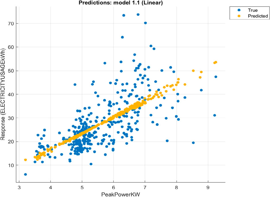
FIGURE 12. Linear prediction model utilizing electricity usage and peak power.

TABLE 4

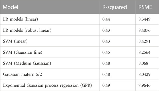
TABLE 4. Regression models and their goodness of fit.

For Linear model Poly5 as shown in Eq. 13 is applied:

$f\left(x\right)=p{1}^{\ast }\widehat{x}5+p{2}^{\ast }\widehat{x}4+p{3}^{\ast }\widehat{x}3+p{4}^{\ast }\widehat{x}2+p{5}^{\ast }x+p6(13)$

Coefficients (with 95% confidence bounds):

p1 = 0.2242 (0.08935, 0.359).

p2 = −6.9 (−11.11, −2.694).

p3 = 82.27 (30.85, 133.7).

p4 = −474.6 (−782, −167.2).

p5 = 1331 (433.5, 2230).

p6 = −1441 (−2465, −417.4).

Where p1, p2, p3, p4, p5, p6 represent the regression coefficients. It can be determined that the greater the polynomial degree, the greater the goodness of fit between the daily electricity usage and peak power and indicates a linear regression fit between electricity usage and peak power.

According to the results, the regression modeler with the best goodness of fit between the parameters of daily electricity usage and peak power was discovered to be exponential GPR. From Table 4 the Exponential GPR model had the greatest R-squared of all the test models at 0.49, while the LR model (robust linear) had the lowest R-squared at 0.43.

3.1.4 Time series

A brief time series analysis was conducted on the dataset to identify the daily energy patterns that reveal energy forecasting coefficients. Figure 13 represents the yearly metered and forecasted daily peak power.

FIGURE 13

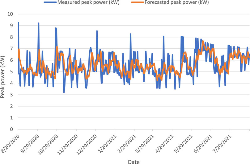
FIGURE 13. Metered and forecasted daily peak power.

The dataset revealed a repeating cycle or trend in the daily peak power in the residential household. Analysis of the SPSS program revealed that the SARIMA model is the most accurate model for the dataset. The model statistics reveal that the RSME, MAPE, and R² were found to be 0.969, 13.222, and 0.633 respectively. Furthermore, the descriptive statistics of the observed data indicate that the mean, maximum, and minimum were 5.5752 kW, 9.2491, and 3.1995 kWh, respectively. On the other hand, the forecasted model statistics indicate that the mean, maximum, and minimum energy usage as 5.574 kW, 7.664 kW, and 4.246 kW, respectively.

3.2 Microgrid solar PV system

The key parameters assessed in the simulation study in MATLAB/Simulink were solar PV power generation, DC bus voltage, battery SOC, and THD.

3.2.1 Energy flow in microgrid system through fuzzy logic control

A control system is utilized to manage the power flow of the microgrid system. The core aim of the control system is to maintain the desired DC bus voltage necessary for the continuous power supply to the electrical loads in a settlement. The energy flow in a grid-connected microgrid system occurs between the solar PV system, BESS, and the utility grid. Therefore, the primary energy supplier to the microgrid system is the solar PV system. The fuzzy logic control (FLC) algorithm was utilized to maintain power between the PV unit, battery, and utility grid. The FLC operates as a supervisory control to inform the charging and discharging of the battery depending on the amount of solar PV power generated (Devi and Mahesh, 2017). Control systems are characterized by using one physical component to change another so that it exhibits desired attributes. The basic components of the FLC framework are a fuzzifier, a fuzzy inference engine in which the ruleset runs, and a defuzzifier. The FLC structure consists of crisp input quantities with either a value of 0 or 1 (Torres-García et al., 2021). The crispy quantities are transformed into fuzzy quantities throughout the fuzzification process. The elements of fuzzy quantities have a degree of membership in a set. The fuzzy logic utilizes a set of if-then rules to execute commands. The defuzzification process then converts the fuzzy quantities into crisps quantities. The defuzzification technique converts the fuzzy sets’ membership degree into real values (Nebey et al., 2020). The deffuzified values present as action commands in a control system. The FLC structure also comprises of input and output variables. Figure 14 shows a process flowchart of the fuzzy logic control structure.

FIGURE 14

FIGURE 14. FLC structure.

The input variables for the fuzzy logic will be the change in power and the change in battery SOC, while the output will be a current reference ($I_{ref}$). The current reference generated informs the grid-connected inverter to discharge power from the grid and when to charge the grid with the excess solar PV power produced. The primary purpose of the FLC is to maintain the desired DC bus voltage of 835 V required by the loads. The current reference generated by the FLC sends a control signal to the components of the microgrid, such as a solar photovoltaic system, a battery, or an electric grid to discharge or charge power in the microgrid bus to achieve the desired bus voltage. The data range of the SOC of the battery is set as the input range of the desired. Eqs 14 and (15) show the mathematical expressions for the input SOC.

${SOC}_{\mathit{min}}\le {SOC}_{\left(t\right)}\le {SOC}_{\mathit{max}}(14)$

$∆SO{C}_{\left(t\right)}={SOC}_{original\left(t\right)}-{SOC}_{now\left(t\right)}(15)$

Where ${SOC}_{\mathit{min}}$ and ${SOC}_{\mathit{max}}$ represent the minimum and maximum SOC of the battery. The charging and discharging of the battery are relative to the time of day. To determine the change in SOC ($∆SO{C}_{\left(t\right)}$), the difference between the original SOC and the actual SOC of the battery is computed. Then, the power balance Equation is expressed mathematically in Eq. (16):

$∆P_{balance}=P_{pv}-P_{load}(16)$

Where $P_{pv}$ and $P_{load}$ represent the solar PV power generated and the load demand power, respectively. Where $∆P_{balance}$ represents the power balance in the microgrid system. When the $∆P_{balance}$ is positive, excess solar PV power is used to charge the battery. The extra electricity generated by the solar PV system is fed into the grid once the battery is fully charged. The fuzzification process involves converting a crips input into a linguistic variable as per the assigned membership functions. The range of values of the inputs was given membership function terms to enable the rules execution of the logic algorithm. The membership functions of fuzzy variables are Negative Big (NB), Negative Small (NS), Zero (ZO), Positive Small (PS), Positive Big (PB).

3.2.2 Rules

The interference engine is instructed by a list of rules that occur based on IF statements between the two inputs being $∆P_{balance}\&∆SO{C}_{\left(t\right)}$.Table 5 illustrates the list of rules for the FLC algorithm.

TABLE 5

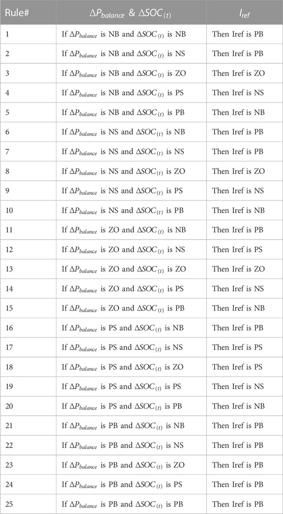
TABLE 5. List of the 25 rules for the FLC.

The result of the $∆P_{balance}$ and $∆SO{C}_{\left(t\right)}$ generates a signal to the grid-connected inverter to relay the power exchange between the microgrid and the grid. As a result, during high peak solar generation hours, the battery SOC increases, and the PCC is disconnected. Still, during low solar generation hours, the grid supplies energy to the electrical loads while charging the battery.

3.2.3 Irradiation profile

Figure 15 depicts the input solar irradiation daily profile for the simulation on MATLAB/Simulink.

FIGURE 15

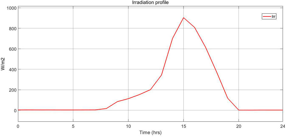
FIGURE 15. Solar irradiation profile.

3.2.4 Solar PV power generation

A graph of the ideal solar PV power generated, and the actual solar PV power generated was prepared. Peak solar irradiation hour (1500 hs) corresponded to 222.5293 kW and 222.2798 kW for the ideal PV and actual PV power, respectively.

Figure 16 indicates the correlation between the ideal solar PV power and the true PV power generated. The ideal PV and real PV peaks were respectively 222.5293 kW and 222.2798 kW during the peak solar irradiation time (1500 hs).

FIGURE 16

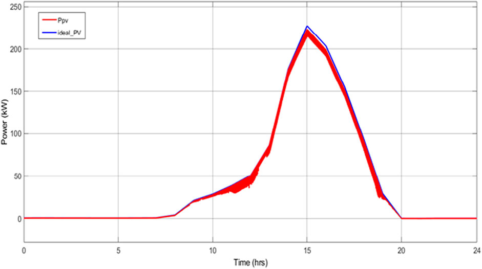
FIGURE 16. Actual (Ppv) and ideal (Pmpp) solar PV power generation.

3.2.5 Battery SOC

Figure 17 depicts the battery SOC (percentage) on the y-axis and time on the x-axis (hrs.).

FIGURE 17

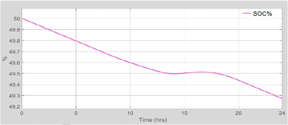
FIGURE 17. Battery SOC.

According to Figure 15 there is virtually little solar PV power generation between 0000 hs and 0900 hs. Therefore, the battery will discharge to power the electrical loads, as depicted in Figure 16. The significant rise in solar insolation between 0900 hs and 1500 hs corresponds to the solar PV power generation. The battery SOC charges and discharges in response to the solar insolation received and the load demand in the microgrid system.

3.2.6 Total harmonic distortion (THD)

Another parameter that was assessed was the THD experienced in the inverter-grid side current. Figure 18 provides a schematic diagram for the THD.

FIGURE 18

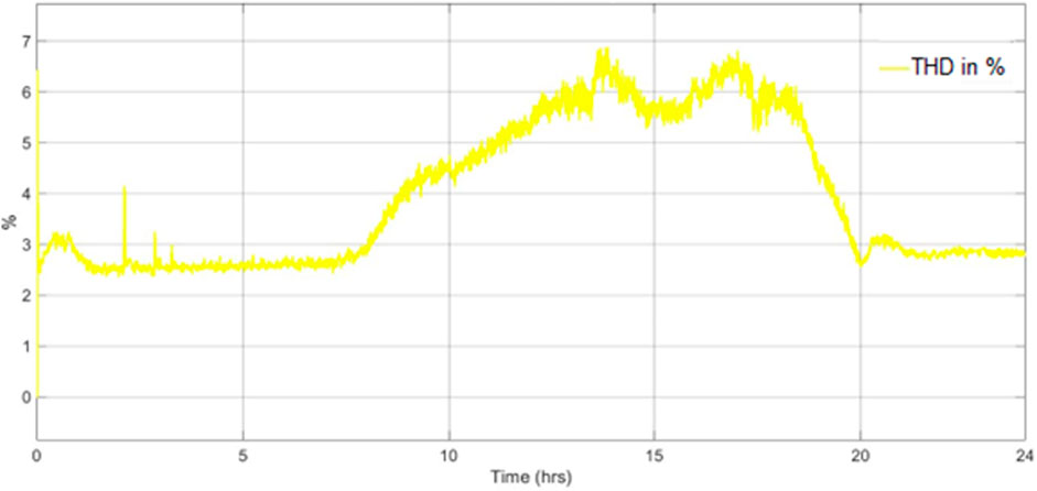
FIGURE 18. Total harmonic distortion (THD).

According to Figure 18, the THD-generated peak was around 6.5%, while the trough was at 2.5%.

3.3 Fuzzy logic control optimized

Graphs were created to demonstrate the impact of using FLCs instead of PID controllers in the power management strategy for the microgrid system. Figure 19 depicts the daily PV power generated and the battery SOC.

FIGURE 19

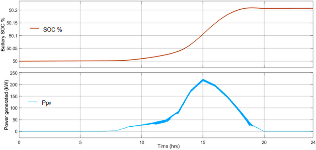
FIGURE 19. Daily PV power generated and the battery SOC.

Figure 19 shows the utility grid supplies power to the electrical loads while charging the battery. The battery stabilizes the DC bus voltage for the microgrid system during the transition from island mode to grid-connected mode. The microgrid system will be in island mode with battery support between 1400 hs and 1600 hs. When the solar PV power generation decreases after 1600 h s, the battery supplies auxiliary power to the electrical loads until the connection to the utility grid is restored. Following that, around 2000 h, when solar PV power generation was at its lowest, the microgrid system began to operate in grid-connected mode. Figure 20 illustrates the THD experienced in the grid-side current inverter.

FIGURE 20

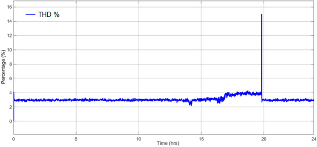
FIGURE 20. THD experienced in the grid-side inverter current.

From Figure 20, it can be observed that the average THD percentage recorded was approximately 3%. By optimizing the microgrid system through FLC, the generated THD was more stable and closer to the allowable THD within 5% as per IEEE-519 standard. The momentary spike in the THD at 2000 hs was due to the transition from the island to a grid-connected mode of operation. The FLC optimization indicated a more stable THD with fewer spikes, which improved the stability of the microgrid system.

4 Conclusion

Solar microgrid systems in residential areas of developing countries have the potential to provide affordable and sustainable electricity. This work has modelled and simulated a solar PV microgrid system for a home in Palapye, Botswana. Load metering analysis and advanced control algorithms utilized in this study indicated that the energy consumption patterns in residential areas vary significantly. Regression models with RMSE values ranging from 0.43 to 0.49 accurately matched the dataset. Control algorithms were developed to address the unpredictability of renewable energy generation and enhance energy efficiency.

The daily performance of a 250-kW peak load solar PV microgrid with PID controllers maintained the DC bus voltage at 835 V for the community load. The battery served as a backup power source during mode switches. The grid-inverter current’s THD ranged from 3% to 7%, complying with the IEEE-519 standard of 5%–7%. FLC algorithm was implemented to maintain a THD of 3% throughout the day. However, the transition from island to grid-connected mode temporarily increased THD, indicating the need for further research on the influence of FLC on the microgrid system. Additional technologies, such as linear programming, are required to address power quality issues in microgrids. Based on the system performance, application of load metering, accurate modelling, and FLC in developing reliable and efficient microgrid systems yields a dependable and sustainable energy supply.

Data availability statement

The raw data supporting the conclusion of this article will be made available by the authors, without undue reservation.

Author contributions

TS: Conceptualization, Investigation, Writing–original draft. RS: Supervision, Conceptualization, Writing–original draft, Writing–review and editing, Validation. MO: Supervision, Writing–review and editing. AY: Software, Writing–original draft. PM: Supervision, Writing–review and editing. GG: Investigation, Writing–review and editing. MK: Resources, Software, Writing–review and editing. NL: Resources, Software, Writing–review and editing. HS: Resources, Software, Writing–review and editing.

Funding

The authors acknowledge Botswana International University of Science and Technology, Palapye, Botswana and SolaNetwork Project, which was funded through the “Innovate UK: Energy Catalyst Round 6: Transforming Energy Access Fund” (Grant reference number: 105280) for supporting the research.

Conflict of interest

The authors declare that the research was conducted in the absence of any commercial or financial relationships that could be construed as a potential conflict of interest.

Publisher’s note

All claims expressed in this article are solely those of the authors and do not necessarily represent those of their affiliated organizations, or those of the publisher, the editors and the reviewers. Any product that may be evaluated in this article, or claim that may be made by its manufacturer, is not guaranteed or endorsed by the publisher.

References

Abdi, H., Mohammadi-ivatloo, B., Javadi, S., Reza Khodaei, A., and Dehnavi, E. (2017). “Distributed generation systems,” in Energy storage systems.

Google Scholar

Ahmed, A., and Abdelhalim, A. Z. (2012). Simulation and implementation of grid-connected inverters. Int. J. Comput. Appl. 60 (4), 0975. doi:10.5120/9683-4117

CrossRef Full Text | Google Scholar

Al-Sakkaf, S., Kassas, M., Khalid, M., and Mohammad, A. A. (2019). An energy management system for residential autonomous DC microgrid using optimized fuzzy logic controller considering economic dispatch. Energies 12 (8), 1457. doi:10.3390/en12081457

CrossRef Full Text | Google Scholar

Alvarez, G., Moradi, H., Smith, M., and Ali, Z. (2018). Modeling a grid-connected PV/battery microgrid system with MPPT controller. Int. Conf. Comput. Inf. Sci. ICCIS 46, 2941.

Google Scholar

Alzahrani, A. I., Mahmud, I., Ramayah, T., Alfarraj, O., and Alalwan, N. (2017). Extendingthe theory of planned behavior (TPB) to explain online game playing among Malaysianundergraduate students. Telematics Inf. 34 (4), 239–251. doi:10.1016/j.tele.2016.07.001

CrossRef Full Text | Google Scholar

Aurangzeb, K. (2019). “Short term power load forecasting using machine learning models for energy management in a smart community,” in International Conference on Computer and Information Sciences, ICCIS, Aljouf, Kingdom of Saudi Arabia, April 10–11, 2019, 1–6.

CrossRef Full Text | Google Scholar

Bellia, H., Youcef, R., and Fatima, M. (2014). A detailed modeling of photovoltaic module using MATLAB. NRIAG J. Astronomy Geophys. 3 (1), 53–61. doi:10.1016/j.nrjag.2014.04.001

CrossRef Full Text | Google Scholar

Bila, M., Opathella, C., and Venkatesh, B. (2016). Grid connected performance of a household lithium-ion battery energy storage system. J. Energy Storage 6, 178–185. doi:10.1016/j.est.2016.04.001

CrossRef Full Text | Google Scholar

Bramareswara Rao, S. N. V., Pavan Kumar, Y. V., Amir, M., and Ahmad, F. (2022). An adaptive neuro-fuzzy control strategy for improved power quality in multi-microgrid clusters. IEEE Access 10, 128007–128021. doi:10.1109/access.2022.3226670

CrossRef Full Text | Google Scholar

Cagnano, A. E. D. T. a. P. M., De Tuglie, E., and Mancarella, P. (2020). Microgrids: overview and guidelines for practical implementations and operation. Appl. Energy 258, 114039. doi:10.1016/j.apenergy.2019.114039

CrossRef Full Text | Google Scholar

Chen, C., Marcel, H., Xingfeng, Si, Wang, Y., and Ding, P. (2018). Characteristics of 36 study islands in the thousand island lake. PANGAEA 10 (1). doi:10.1594/PANGAEA.885960

CrossRef Full Text | Google Scholar

Chou, J. S., and Duc Son, T. (2018). Forecasting energy consumption time series using machine learning techniques based on usage patterns of residential householders. Energy 165, 709–726. doi:10.1016/j.energy.2018.09.144

CrossRef Full Text | Google Scholar

Dabla, N. (2021). Renewables readiness assessment: Botswana. Masdar City, United Arab Emirates: IRENA.

Google Scholar

Deb, C., Zhang, F., Yang, J., Lee, S. E., and Shah, K. W. (2017a). A review on time series forecasting techniques for building energy consumption. Renew. Sustain. Energy Rev. 24 (74), 902–924. doi:10.1016/j.rser.2017.02.085

CrossRef Full Text | Google Scholar

Deb, C., Zhang, F., Yang, J., Lee, S. E., and Shah, K. W. (2017b). A review on time series forecasting techniques for building energy consumption. Renew. Sustain. Energy Rev. 74, 902–924. Elsevier. doi:10.1016/j.rser.2017.02.085

CrossRef Full Text | Google Scholar

Devi, B. G., and Mahesh, M. (2017). A brief survey on different multilevel inverter topologies for grid-tied solar photo voltaic system. IEEE Int. Conf. Smart Energy Grid Eng. (SEGE), 51–55. doi:10.1109/SEGE.2017.8052775

CrossRef Full Text | Google Scholar

Dw, G. (2015). Energy storage for sustainable microgrid. Massachusetts, United States: Academic Press.

Google Scholar

Farrokhabadi, M., Sebastian, K., ClaudioCañizares, A., Bhattacharya, K., and Leibfried, T. (2018). Battery energy storage system models for microgrid stability analysis and dynamic simulation. IEEE Trans. Power Syst. 33 (2), 2301–2312. doi:10.1109/tpwrs.2017.2740163

CrossRef Full Text | Google Scholar

Hasan, M. A., and Bin Arif, M. S. (2018). Microgrid architecture, control, and operation. Hybrid-Renewable Energy Syst. Microgrids, 24–36. doi:10.1016/B978-0-08-102493-5.00002-9

CrossRef Full Text | Google Scholar

Hasiah, S., Ghapur, E. A., Aziz, N. A. N., Dhafina, W. A., Hamizah, A., Laily, A. R. N., et al. (2014). Study the electrical properties and the efficiency of polythiophene with dye and chlorophyll as bulk hetero-junction organic solar cell. Adv. Mater. Res. 895, 513–519. doi:10.4028/www.scientific.net/amr.895.513

CrossRef Full Text | Google Scholar

Hu, J., Shan, Y., Guerrero, J. M., Adrian, I., Chan, K. W., and Rodriguez, J. (2020). Model predictive control of microgrids – an overview. Renew. Sustain. Energy Rev. 136, 110422. doi:10.1016/j.rser.2020.110422

CrossRef Full Text | Google Scholar

IRENA (2022). Renewable energy market analysis: Africa and its regions. IRENA. Available at: www.irena.org/publications.

Google Scholar

Justo Jackson, J., Mwasilu, F., Lee, Ju, and Jin, W. J. (2013). AC-microgrids versus DC-microgrids with distributed energy resources: a review. Renew. Sustain. Energy Rev. 24, 387–405. doi:10.1016/j.rser.2013.03.067

CrossRef Full Text | Google Scholar

Kabiri, R., Holmes, G., and Mcgrath, B. (2013). “DigSILENT modelling of power electronic converters for distributed generation networks,” in PowerFactory Users’ Conference and Future Networks Technical Seminar, Sydney-Australia, 5-6th September 2013.

Google Scholar

Kondrath, N. (2018). An overview of bidirectional DC-DC converter topologies and control strategies for interfacing energy storage systems in microgrids. J. Electr. Eng. 6, 11–17. doi:10.17265/2328-2223/2018.01.002

CrossRef Full Text | Google Scholar

Kularatna, N. (2015). “Energy storage devices for electronic systems,” in Rechargeable batteries and supercapacitors (University of Waikato Hamilton).

Google Scholar

Kuster, C., Rezgui, Y., and Mourshed, M. (2017). Electrical load forecasting models: a critical systematic review. Sustain. Cities Soc. 35, 257–270. doi:10.1016/j.scs.2017.08.009

CrossRef Full Text | Google Scholar

Lee, Ji, Han, B., Choi, N., Jeong, Y. S., Yang, H. S., and Cha, H. J. (2011). DC micro-grid operational analysis with a detailed simulation model for distributed generation. J. Power Electron. 11 (3), 350–359. doi:10.6113/jpe.2011.11.3.350

CrossRef Full Text | Google Scholar

Leonori, S., De Santis, E., Rizzi, A., and Frattale Mascioli, F. M. (2016). Optimization of a microgrid energy management system based on a fuzzy logic controller. IECON Proc. Ind. Electron. Conf. 20, 6615. doi:10.1109/IECON.2016.7793965

CrossRef Full Text | Google Scholar

Li, W., and Joós, G. (2007). Comparison of energy storage system technologies and configurations in a wind farm. IEEE Power Electron. Spec. Conf., 1280–1285. doi:10.1109/PESC.2007.4342177

CrossRef Full Text | Google Scholar

Mahlooji, M. H., Mohammadi, H. R., and Rahimi, M. (2013). A review on modeling and control of grid-connected photovoltaic inverters with LCL filter. Renew. Sustain. Energy Rev. 81, 563–578. doi:10.1016/j.rser.2017.08.002

CrossRef Full Text | Google Scholar

Nebey, A. H., Taye, B. Z., and Workineh, T. G. (2020). GIS-based irrigation dams potential assessment of floating solar PV system. J. Energy 2020, 1–10. doi:10.1155/2020/1268493

CrossRef Full Text | Google Scholar

Nelson, F., and Biswas, M. A. R. (2015). Regression analysis for prediction of residential energy consumption. Renew. Sustain. Energy Rev. 47, 332–343. Elsevier. doi:10.1016/j.rser.2015.03.035

CrossRef Full Text | Google Scholar

Ngoc Nam, N., Choi, M., and Il Lee, Y. (2019). Model predictive control of a grid-connected inverter with LCL filter using robust disturbance observer. IFAC Workshop Control Smart Grid Renew. Energy Syst. CSGRES 52, 135–140. doi:10.1016/j.ifacol.2019.08.168

CrossRef Full Text | Google Scholar

Obaro, A., Munda, J. L. M., and Adedamola Yusuff, A. (2023). Modelling and energy management of an off-grid distributed energy system: a typical community scenario in South Africa. Energies 16 (2), 693. doi:10.3390/en16020693

CrossRef Full Text | Google Scholar

Olivier TremblayLouis, A., and DessaintLouis, D.A.-I. D. (2007). “A generic battery model for the dynamic simulation of hybrid electric vehicles,” in Vehicle power and propulsion conference.

CrossRef Full Text | Google Scholar

Palaniappan, K., Veerapeneni, S., Cuzner, R., and Zhao, Y. (2017). “Assessment of the feasibility of interconnected smart DC homes in a DC microgrid to reduce utility costs of low income households,” in IEEE 2nd International Conference on Direct Current Microgrids, ICDCM, Nuremburg, Germany, 27-29 June 2017, 467–730.

CrossRef Full Text | Google Scholar

Phuong, Le M., Dzung, P. Q., and Minh Huy, N. (2015). Science and technology development. Ho Chi Minh city, Vietnam: University of Technology,VNU-HCM. vol. 15, no. K3.

Google Scholar

Qazi, S. (2017). “PV systems affordability, community solar, and solar microgrids,” in Standalone photovoltaic (PV) systems for disaster relief and remote areas, 177–202.

CrossRef Full Text | Google Scholar

Rahimi, B., Nadri, H., Afshar, H. L., and Timpka, T. (2018). A systematic review of the technology acceptance model in health informatics. Natl. Libr. Med. 9 (3), 604–634. doi:10.1055/s-0038-1668091

PubMed Abstract | CrossRef Full Text | Google Scholar

Ravi, S., Oladiran, T., Gamariel, G., Makepe, P., Keisang, K., and David Ladu, N. S. (2022). An assessment and design of a distributed hybrid energy system for rural electrification: the case for Jamataka village, Botswana. Int. Trans. Electr. Energy Syst. 5, 1–12. doi:10.1155/2022/4841241

CrossRef Full Text | Google Scholar

Reyes-García, C. A., and Torres-Garcia, A. A. (2022). “Fuzzy logic and fuzzy systems,” in Biosignal processing and classification using computational learning and intelligence principles, algorithms, and applications (Academic Press), 153–176.

Google Scholar

Ridwana, I., Nassif, N., and Choi, W. (2020). Modeling of building energy consumption by integrating regression analysis and artificial neural network with data classification. Buildings 10 (1–14), 198. doi:10.3390/buildings10110198

CrossRef Full Text | Google Scholar

Shezan, Sk. A., Fatin Ishraque, Md., Shafiullah, G. M., Kamwa, I., Paul, L. C., Muyeen, S. M., et al. (2023). Optimization and control of solar-wind islanded hybrid microgrid by using heuristic and deterministic optimization algorithms and fuzzy logic controller. Energy Rep. 10, 3272–3288. doi:10.1016/j.egyr.2023.10.016

CrossRef Full Text | Google Scholar

Singh, P. K., Rajak, P. K., Singh, V. K., Singh, M. P., Naik, A. S., and Raju, S. V. (2016). Studies on thermal maturity and hydrocarbon potential of lignites of Bikaner–Nagaur basin, Rajasthan. Energy Explor. Exploitation 34 (1), 140–157. doi:10.1177/0144598715623679

CrossRef Full Text | Google Scholar

Singh, S., and Yassine, A. (2018). Big data mining of energy time series for behavioral analytics and energy consumption forecasting. Energies 11 (2), 452. doi:10.3390/en11020452

CrossRef Full Text | Google Scholar

Situmbeko, S. M. (2018). Towards a sustainable energy future for sub-saharan Africa. Energy Manag. Sustain. Dev., 48–66. doi:10.5772/intechopen.75953

CrossRef Full Text | Google Scholar

sley, A. W. F. a. C. A. (2021). Cost projections for utility-scale battery storage: 2021 update. CO, United States: National Renewable Energy Laboratory NREL.

Google Scholar

Srivastava, R., Amir, M., Ahmad, F., Agrawal, S. K., Dwivedi, A., and Yadav, A. K. (2022). Performance evaluation of grid connected solar powered microgrid: a case study. Front. Energy Res. 10, 1044651. doi:10.3389/fenrg.2022.1044651

CrossRef Full Text | Google Scholar

Tajjour, S. a. S. S. C., and Singh Chandel, S. (2023). A comprehensive review on sustainable energy management systems for optimal operation of future-generation of solar microgrids. Sustain. Energy Technol. Assessments 58, 103377. doi:10.1016/j.seta.2023.103377

CrossRef Full Text | Google Scholar

Torres-García, A. A., Reyes-García, C. A., Villaseñor-Pineda, L., and Mendoza-Montoya, O. (2021). “Principles, algorithms, and applications,” in Biosignal processing and classification using computational learning and intelligence (Elsevier).

Google Scholar

U. E. I. Administration (2019). International energy outlook 2019 international energy outlook 2019. Washington DC: International Energy Agency.

Google Scholar

Vetter, M., and Rohr, L. (2014). “Lithium-ion batteries for storage of renewable energies and electric grid backup,” in Lithium-ion batteries advances and applications (Elsevier), 293–309.

CrossRef Full Text | Google Scholar

Zhang, S., Yao, L., Sun, A., and Tay, Yi (2018). Deep learning based recommender system: a survey and new perspectives. ACM Comput. Surv. 1 (1), 1–38. doi:10.1145/3285029

CrossRef Full Text | Google Scholar

Zhang, X. M., Grolinger, K., Miriam, A., Capretz, M., and Seewald, L. (2019). “Forecasting residential energy consumption: single household perspective,” in Proceedings - 17th IEEE International Conference on Machine Learning and Applications, ICMLA, Orlando, FL, USA, December 17-20, 2018, 110–170.

Google Scholar