Optimal scheduling for charging and discharging of electric vehicles based on deep reinforcement learning

1 Introduction

Electric vehicles (EVs), with their outstanding advantages of being clean, environmentally friendly, and low noise, have become the focus of industries around the world. However, as the scale of EVs continues to expand, their high charging demand is gradually increasing its proportion within the power system, posing significant challenges to the stability and safety of the smart grid (Chen et al., 2021; Chen et al., 2023). The behavior of EV owners directly influences the spatiotemporal distribution of charging demand, introducing uncertainties in charging time and power for EVs. These uncertainties could have a significant impact on the normal operation and precise control of the smart grid (Wen et al., 2015; Liu et al., 2022). Simultaneously, EVs can act as an excellent mobile energy storage device and can serve as a distributed power source to supplement the power system when necessary. This capability creates a source-load complementary intelligent power dispatch strategy (Lu et al., 2020). Therefore, it is imperative to manage the charging and discharging of EVs. A rational charging and discharging strategy will not only effectively mitigate the adverse effects of charging behavior on the grid load but also play a positive role in peak shaving, load stabilization, and interaction with the grid (Zhao et al., 2011).

Traditional methods for optimizing the scheduling of EV charging and discharging are divided into three main categories: methods based on dynamic programming, methods based on day-ahead scheduling, and model-based methods (Zhang et al., 2022). However, the application of traditional algorithms to the optimization of EV charging scheduling faces two major challenges: the massive number of EVs results in high-dimensional scheduling optimization variables, often leading to the ’curse of dimensionality’ (Shi et al., 2019); the fluctuations within the energy system and the uncertainty of EV user demand make it difficult to establish accurate models, limiting the control effectiveness and performance of the algorithm.

Reinforcement learning methods, which can obtain optimal solutions to sequential decision-making problems without explicitly constructing a complete environment model, have been widely deployed in addressing the charging scheduling problem of EVs. Deep reinforcement learning-based charging scheduling methods can be divided into two categories: value-based algorithms and policy-based algorithms (Xiong et al., 2021). Regarding value-based algorithms (Liu et al., 2019), developed an incremental update-based flexible EV charging strategy. This approach considers the user experience of EV drivers and aims to minimize their charging costs (Vandael et al., 2015). sought to learn from transitional samples and proposed a batch reinforcement learning algorithm. This method ultimately resulted in the optimal charging strategy for reducing charging costs (Wan et al., 2018). innovatively used a long short-term memory (LSTM) network to extract electricity price features. They described the scheduling of EV charging and discharging as a Markov decision process (MDP) with unknown probabilities, eliminating the need for any system model information.

Value-based algorithms are suitable only for discrete action spaces, while policy-based algorithms can handle continuous action spaces (Nachum et al., 2017; Jin and Xu, 2020) proposed an intelligent charging algorithm based on actor-critic (AC) learning. This method successfully reduced the dimensionality of the state variables for optimization in EVs (Zhao and Hu, 2021). employed the TD3 algorithm for modeling and introduced random noise into the state during the training of the intelligent agent. This approach achieved generalized control capability over the charging behavior of EVs under various states (Ding et al., 2020). established an MDP model to characterize uncertain time series, thereby reducing the system’s uncertainty. They subsequently employed a reinforcement learning technique based on the deep deterministic policy gradient (DDPG) to solve for a charging and discharging scheduling strategy that maximizes profits for the distribution network.

Currently, the main challenge facing reinforcement learning algorithms for optimizing EV charging and discharging is the issue of algorithm non-convergence caused by the high-dimensional variable characteristics in the multi-agent environment (Pan et al., 2020). utilized the approximate dynamic programming (ADP) method to generalize across similar states and actions, reducing the need to explore each possible combination exhaustively. However, the ADP method requires manual design and feature selection, which is less automated compared to deep reinforcement learning (DRL) (Long et al., 2019). formulated the EV clusters charging problem as a bi-level Markov Decision Process, breaking down complex tasks to enhance convergence and manage high dimensions. However, its hierarchical structure can hinder end-to-end learning, potentially leading to suboptimal strategies, unlike DRL which can map states directly to actions. Therefore, this paper proposes a reinforcement learning algorithm specifically for the optimal scheduling of EV charging and discharging. The algorithm integrates LSTM and MADDPG, where LSTM is utilized to extract features from historical electricity prices, and MADDPG is employed to formulate charging and discharging strategies. This algorithm aims to solve the problem of non-convergence in multi-agent environments while also fully utilizing historical time-of-use electricity price data to aid the agent in decision-making. The major contributions of this paper are as follows.

• This paper establishes a model for optimizing the scheduling of EV charging and discharging in a multi-agent environment. The model involves the power grid, charging equipment, and EVs, and the flow of electricity and information is controlled by different entities. Besides, the charging control model is characterized as a partially observable Markov decision process (POMDP).

• This paper sets the optimization objective of the algorithm by considering three main factors: the cost of charging and discharging, the impact of EV charging and discharging on the grid load, and users’ usage requirements. Corresponding constraint conditions of above objectives are also provided.

• This paper introduces the long short-term memory enhanced multi-agent deep deterministic policy gradient (LEMADDPG) algorithm to obtain the optimal scheduling strategy of EVs. The LSTM network is utilized to extract features from the TOU electricity price data in order to guide the EV exploring the optimal charging and discharging action strategy.

• Complete simulation results prove that the proposed LEMADDPG algorithm can obtain the fastest convergence speed, the smallest fluctuation and the highest cumulative reward compared with the DDPG and deep Q-network (DQN) algorithms. In addition, results also indicate that the LSTM network can extract features of time-of-use electricity price data and make reasonable predictions for future prices.

2 Scheduling model

The electrical usage scenario in this paper is a smart residential community. This community consists of multiple households that own electric vehicles. Ample charging devices are installed throughout the area for EV usage. In the process of charging and discharging, users can determine the duration themselves. Aside from purchasing electricity to charge their EVs, users can also use their vehicles as home energy storage devices to sell excess electricity back to the grid.

This paper establishes a simple EV charging and discharging optimization scheduling model, as shown in Figure 1. The model involves three primary components: the power grid, charging equipment, and electric vehicles. Specifically, the power grid is responsible for providing electrical supply and real-time time-of-use price information. The charging equipment fulfills the role of purchasing electricity from the grid based on the needs of EVs and then distributing this electricity to the vehicles. It also transfers price information to EVs and the current status of the vehicles to the grid system. Electric vehicles are managed to charge or discharge based on real-time price information and provide feedback to the charging equipment about their current state information. The scheduling process can be divided into three steps: information collection, real-time decision-making, and command sending. First, the decision-making unit collects information on electricity prices provided by the grid, demand information, and the battery status of the EVs. Next, the decision-making unit inputs the collected status information into the decision network and outputs the charging and discharging plans for each EV. Finally, upon receiving the commands, the grid dispatches the corresponding electricity to various charging devices, completing the energy scheduling for that time period.

FIGURE 1

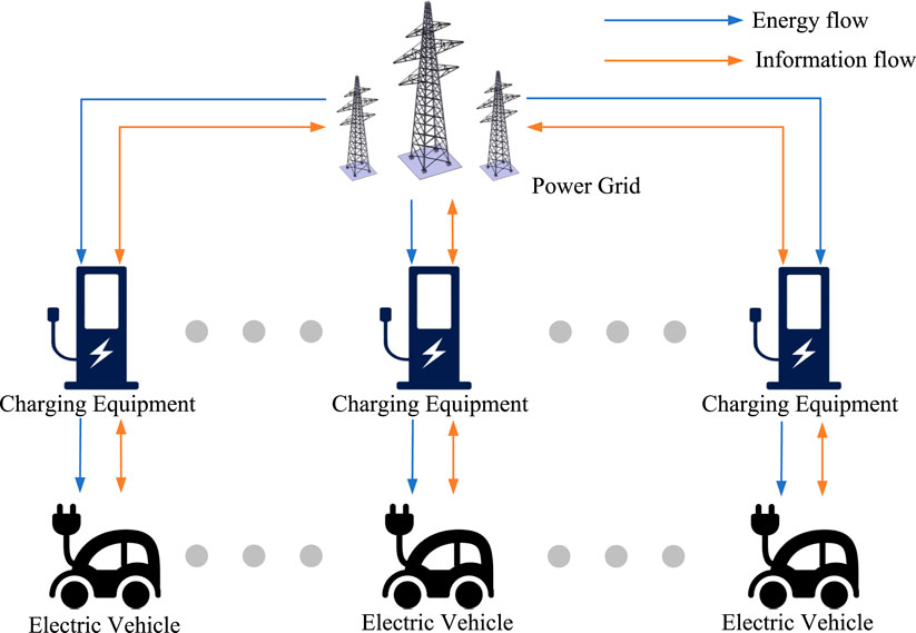
FIGURE 1. Diagram of charging and discharging scheduling for EVs.

2.1 Basic assumptions

In the community, there are a total of N EVs. The set of EVs is designated as B = {1, …, i, …, N}. It is assumed that EVs start charging and discharging immediately after being connected to the charging equipment. The scheduling process only considers EVs in the state of charging and discharging. A scheduling period is set as 24 h, with a scheduling step of 1 h. The set of time slots is designated as H = {1, …, t, …, 24}.

In each scheduling step, EVs are divided into online and offline states. The set of online time slots for EV i is denoted as $T_i^{\text{online}}=\{T_i^{\text{start}},\dots ,t,\dots ,T_i^{\text{end}}\},0\le T_i^{\text{start}}\le t\le T_i^{\text{end}}\le 23$. $T_i^{\text{start}}$ is the time slot when the EV connects to the charging equipment to start charging. $T_i^{\text{end}}$ is the time slot when the EV finishes charging and leaves. Assuming that all EVs arrive or leave at the whole hour, the online time slots should be a continuous set of natural numbers. In other time slots, if EV i is not connected to the charging equipment, it is considered as not participating in the current scheduling.

2.2 Optimization objective

The primary objective of the optimized scheduling for EV charging and discharging is to minimize the cost associated with EV charging and discharging. It also takes into account the impact of the total power of the EV cluster’s charging and discharging activities on the stable operation of the power grid, as well as user usage requirements. Based on the previous assumptions, this paper considers the following cost factors.

2.2.1 Cost of charging and discharging $C_{i,t}^{\mathrm{charge}}$

Under the time-of-use (TOU) pricing policy, the cost of charging and discharging $C_{i,t}^{\text{charge}}$ depends on the current electricity price and the amount of charging and discharging. Thus, the cost generated by charging and discharging behavior can be represented as:

$C_{i,t}^{\text{charge}}={\lambda }_t\cdot l_{i,t}(1)$

where λ_t is the current electricity price during time slot t. l_i,t is the total charging and discharging quantity of EV i in time slot t. It can be specifically expressed as follows:

$l_{i,t}=\left\{\begin{array}{c}\hfill p_{i,t},t\in T_i^{\text{online}}\hfill \\ \hfill 0,t\notin T_i^{\text{online}}\hfill \end{array}\right.(2)$

where p_i,t is the average charging and discharging power of EV i during time slot t. It is positive during charging and negative during discharging. $T_i^{\mathit{online}}$ is the set of online time slots.

2.2.2 Cost of state of charge (SOC) $C_{i,t}^{\mathrm{SOC}}$

The randomness of EV charging behavior mainly manifests as uncertainty in the start time and duration of charging. Furthermore, the state of charge at the start of charging is influenced by the usage and charging habits of the EV user (Kim, 2008). Considering the user’s usage needs for EVs, the state of charge after charging and discharging should meet the user’s upcoming driving needs. To simplify the model, we make the following assumptions:

EVs arrive at the charging equipment to charge at any time within 24 h and leave after several hours of charging. Both the arrival time and departure time follow a uniform distribution, with a probability density function of:

$f\left(t\right)=\left\{\begin{array}{c}\frac{1}{b-a},a\le t\le b\hfill \\ 0,other\hfill \end{array}\right.(3)$

where, a = 0, b = 23.

The initial SOC of EVs follows a normal distribution, with a probability density function of:

$f_{\mathrm{i}\mathrm{n}\mathrm{t}}\left(SOC\right)=\frac{1}{\sigma \sqrt{2\pi }}{e}^{\left[-\frac{{\left(SOC-\mu \right)}^2}{2{\sigma }^2}\right]}(4)$

where μ = 0.5, σ = 0.16.

While the usage needs of a single user are difficult to predict, extensive data shows that user requirements follow a normal distribution. Thus, the usage requirement SOC_ideal also follows a normal distribution, with a probability density function of:

$f_{\text{ideal}}\left(SOC\right)=\frac{1}{\sigma \sqrt{2\pi }}{e}^{\left[-\frac{{\left(SOC-\mu \right)}^2}{2{\sigma }^2}\right]}(5)$

where, μ = 0.5, σ = 0.16.

Based on the above description, the cost of state of charge $C_{i,t}^{\mathit{SOC}}$ incurred to meet user usage needs can be expressed as:

$C_{i,t}^{\text{soc}}=\delta \cdot {\left[E\cdot \left(SO{C}_{\text{ideal}}-SO{C}_{i,T_i^{\text{end}}+1}\right)\right]}^2(6)$

where SOC_ideal represents the user’s expected SOC for an EV. It describes the user’s usage needs. For example, if the user expects to travel a long distance after charging, this value is higher. $SO{C}_{i,T_i^{\text{end}}+1}$ represents the SOC of EV i when it leaves the equipment after charging. δ is the coefficient of the SOC cost, 0 ≤ δ ≤ 1. E is the maximum capacity of the EV battery, determined by the EV model. According to the above formula, if the SOC after charging $SO{C}_{i,T_i^{\text{end}}+1}$ deviates significantly from the user’s expected value SOC_ideal, it will result in a higher penalty cost.

2.2.3 Cost of grid load impact $C_{i,t}^{\mathrm{impact}}$

During the charging and discharging process, EVs’ behaviors impact the load curve of the power grid (Rawat et al., 2019). Based on previous discussions, the power grid system is expected to operate smoothly. This requires certain restrictions on the total charging and discharging power of the EV cluster. Therefore, this paper introduces the impact cost of the EV cluster’s charging and discharging behavior on the power grid, which is represented as:

$C_{i,t}^{\text{impact}}=\left\{\begin{array}{c}\hfill \mu \cdot {\lambda }_t\cdot l_{i,t},l_t\ge l_{th}\hfill \\ \hfill 0,l_t<l_{th}\hfill \end{array}\right.(7)$

where μ denotes the cost coefficient for load impact. λ_t is the current electricity price. l_i,t is the total amount of charging and discharging for EV i in period t. l_t is the total load generated by the EV cluster in period t, defined as:

$l_t={\displaystyle \sum _{i=1}^N}{l}_{i,t}(8)$

The cost of grid load impact is incurred only when the total load of the EV cluster exceeds a certain threshold (Shao et al., 2011). The threshold l_th can be defined as:

$l_{th}=k_{th}\cdot p_{\max }\cdot N(9)$

where k_th represents the percentage threshold of the charging and discharging power of the EV cluster in the current grid load. This threshold limit is set by the power grid system based on recent load conditions and is released to all EVs participating in charging and discharging. p_max is the maximum charging power of the EV cluster, defined as follows:

$p_{\max }=\max \left(p_{i,\max }\right),i\in B(10)$

Based on the above assumptions, we propose the optimization objective to minimize the comprehensive cost C generated in the charging and discharging process. The comprehensive cost C can be defined as:

$\begin{array}{c}minC={\displaystyle \sum _{i=1}^N}\left\{{\displaystyle \sum _{t=1}^{24}}\left[C_{i,t}^{\text{charge}}+C_{i,t}^{\text{soc}}\right]+C_{i,t}^{\text{impact}}\right\}\hfill \\ s.t.\left\{\begin{array}{c}\mathrm{0}\le {\displaystyle \sum _t^T}{C}_{i,t}^{\text{charge}}\le 1,i=\mathrm{1,2},\dots ,N\hfill \\ \mathrm{0}\le {\displaystyle \sum _t^T}{C}_{i,t}^{\text{soc}}\le 1,i=\mathrm{1,2},\dots ,N\hfill \\ \mathrm{0}\le {\displaystyle \sum _t^T}{C}_{i,t}^{\text{impact}}\le 1,i=\mathrm{1,2},\dots ,N\hfill \\ 0\le C\le 3N\hfill \end{array}\right.\hfill \end{array}(11)$

2.3 Constraint condition

The SOC for EV i should satisfy the constraint:

$SO{C}_{\min }\le SO{C}_{i,t}\le SO{C}_{\max }(12)$

Generally, the SOC of an EV is represented as a percentage, with SOC_min = 0%, SOC_max = 100%.

The charging and discharging power of EV i during time period t is subject to the constraint:

$\left|p_{i,t}\right|\le p_{\max ,i},p_{\max ,i}=\min \left(\omega \cdot SO{C}_{i,t},P_{\max }\right)(13)$

where ω is the charging power limit coefficient. P_max is the maximum charging power of EV i, depending on the specific EV model. The real-time charging power of EVs is influenced by both the SOC and the maximum charging power. When the SOC is high, to protect the battery, the EV does not charge and discharge at full power. Instead, it operates at a lower power level based on the current SOC.

3 POMDP model

During the charging and discharging process, each EV agent is unable to acquire a complete observation of the system. They are unaware of the states and actions of other agents. The agent must make charging and discharging decisions that can achieve higher benefits based on their current observations and strategies to obtain the optimal scheduling strategy (Dai et al., 2021). Therefore, in contrast to the general Markov decision process model in reinforcement learning, we describe the charging and discharging optimization scheduling problem in this multi-agent environment as a POMDP model (Loisy and Heinonen, 2023).

State Observation: The state information that EV i can observe at time period t is assumed to be:

$o_{i,t}=\left\{{\lambda }_t,u_{i,t},SO{C}_{i,t}\right\}(14)$

where λ_t is the current TOU electricity price. u_i,t indicates whether EV i is connected to the charging equipment for charging in period t, i.e., the online status of EV. Specifically, it can be represented as:

$u_{i,t}=\left\{\begin{array}{c}\hfill 1,t\in T_i^{\text{online}}\hfill \\ \hfill 0,t\notin T_i^{\text{online}}\hfill \end{array}\right.(15)$

where SOC_i,t is the SOC of EV i in period t.

The system state includes the current state information of all EVs and the current electricity price information. It can be described as the combination of the EV cluster and the current time-of-use price information, which is:

$\begin{array}{ll}\hfill O_t& =\left\{o_{1,t},o_{2,t},\dots ,o_{N,t}\right\}\hfill \\ \hfill & =\left\{{\lambda }_t,u_{1,t},\dots ,u_{N,t},SO{C}_{1,t},\dots ,SO{C}_{N,t}\right\}\hfill \end{array}(16)$

Action: We select the average charging and discharging power p_i,t of EV i in period t as action a_i,t of the agent, that is:

$a_{i,t}=p_{i,t}(17)$

where a_i,t is positive when the EV is charging and negative when discharging.

The agent can charge the EV during low electricity price periods and sell electricity to the grid through the EV battery during peak price periods to obtain economic benefits. The joint action taken by all EV agents in period t is denoted as a_t = {a₁, a₂, …, a_N}.

Reward: Reward is an important factor in evaluating the quality of the action strategies adopted by each agent. Based on the above discussion and the optimization objective of the model, we set the reward as follows:

$r_i=\left\{\begin{array}{c}\hfill r_i^{\text{ch}}+r_i^{\text{punish}}+r_i^{\text{soc}},t=T_i^{\text{end}}\hfill \\ \hfill r_i^{\text{ch}}+r_i^{\text{punish}},t\ne T_i^{\text{end}}\hfill \end{array}\right.(18)$

$r_i^{\text{ch}}$ is the reward for the charging and discharging behavior of EV i, defined as:

$r_i^{\text{ch}}=-{\lambda }_t{a}_{i,t}(19)$

It indicates that high electricity prices and high charging power will reduce the rewards obtained by the agent.

$r_t^{\mathit{punish}}$ is the reward for the total impact on the grid load of the charging and discharging behavior of the EV cluster in time period t, defined as:

$r_t^{\text{punish}}=\left\{\begin{array}{c}\hfill -\rho \cdot {\lambda }_t{a}_{i,t},{\displaystyle \sum _{i=1}^N}{a}_{i,t}\ge l_{th}\hfill \\ \hfill 0,{\displaystyle \sum _{i=1}^N}{a}_{i,t}<l_{th}\hfill \end{array}\right.(20)$

where l_th is the threshold limit of the grid for the total charging and discharging power of the EV cluster. ρ is the load reward conversion factor.

$r_i^{\text{SOC}}$ is the reward for EV i meeting the user’s usage requirements at the end of charging, defined as:

$r_i^{\text{soc}}=-\upsilon \cdot C_{i,t}^{\text{soc}}(21)$

where υ is the SOC reward conversion factor. $C_{i,t}^{\mathit{soc}}$ is the cost of SOC.

State Transition: After the EV agent cluster executes the joint action a_t = {a₁, a₂, …, a_N}, the system state transitions from O_t to O_t+1. Each agent receives the corresponding rewards and state observation information for the next stage from the environment. This transition process can be represented as a function:

$O_{t+1}=f\left(O_t,a_t\right)(22)$

4 LEMADDPG algorithm design

Based on the previous discussion, we modeled the problem of optimizing the charging and discharging schedule of the EV cluster as a POMDP in a multi-agent environment. However, reinforcement learning algorithms in multi-agent environments often face the challenge of environmental instability (Wu et al., 2020). This is due to each agent constantly learning and improving their strategy. From the perspective of a single agent, the environment is in a dynamic state of change, and the agent cannot adapt to the changing environment by simply altering its own strategy. To address this challenge, researchers have begun to focus on multi-agent reinforcement learning methods, aiming to resolve the issue of the non-convergence of reinforcement learning algorithms caused by environmental instability.

Furthermore, extracting discriminative features from raw data is a key method to improve reinforcement learning algorithms. In this problem, we expect a good algorithm to fully utilize the trend information of TOU electricity prices to guide the action selection of agents. It should result in an optimal scheduling strategy that minimizes the overall cost (He et al., 2021; Liao et al., 2021). Since TOU electricity prices fluctuate in a quasi-periodic manner and have a natural time sequence, it is suitable to use past prices to infer future price trends.

Therefore, this paper takes the multi-agent deep deterministic policy gradient (MADDPG) (Lowe et al., 2017) algorithm as the main body and uses the long short-term memory (LSTM) network (Shi et al., 2015) to extract features from the input TOU electricity price data. These feature data are used to guide the EV agent to explore the optimal charging and discharging action strategy. Consequently, we propose the long short-term memory enhanced multi-agent deep deterministic policy gradient (LEMADDPG) algorithm.

4.1 Electricity price feature extraction

LSTM (Shi et al., 2015) is a type of recurrent neural network specifically designed to address the long-term dependency problem that is prevalent in regular recurrent neural networks (RNNs). The key characteristic of LSTM is the introduction of a memory cell, also referred to simply as a cell. The memory cell can retain additional information and controls the flow of information via three gate structures: input gate, forget gate, and output gate. The input gate determines whether to accept new input data. The forget gate decides whether to retain the contents of the old memory cell. The output gate decides whether to output the contents of the memory cell as a hidden state. In this way, LSTM can alleviate the vanishing gradient problem and capture long-distance dependencies in sequences, making it highly suitable for processing and predicting time series data. A typical LSTM network structure is shown in Figure 2.

FIGURE 2

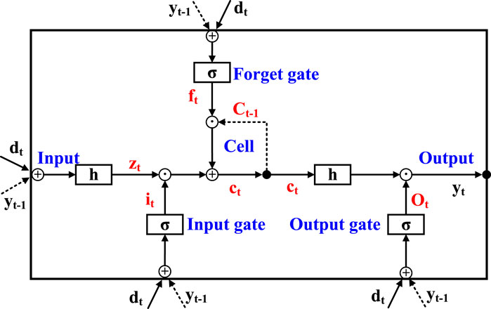
FIGURE 2. LSTM network structure (Wan et al., 2018).

In this paper, before the algorithm starts training, the real historical TOU electricity price data are input into the LSTM network for pre-training. The trained LSTM network can output the extracted electricity price features. Later, during the training process, the LSTM network outputs the corresponding electricity price features based on the current system state to guide the action selection of the agents.

4.2 LEMADDPG algorithm structure

The algorithm adopts the enhanced actor-critic structure (Konda and Tsitsiklis, 1999) from MADDPG, as shown in Figure 3. Each agent includes two types of networks: the policy network (Actor), responsible for making appropriate decision actions based on the current observation information, and the value network (Critic), which evaluates the quality of the actions output by the policy network.

FIGURE 3

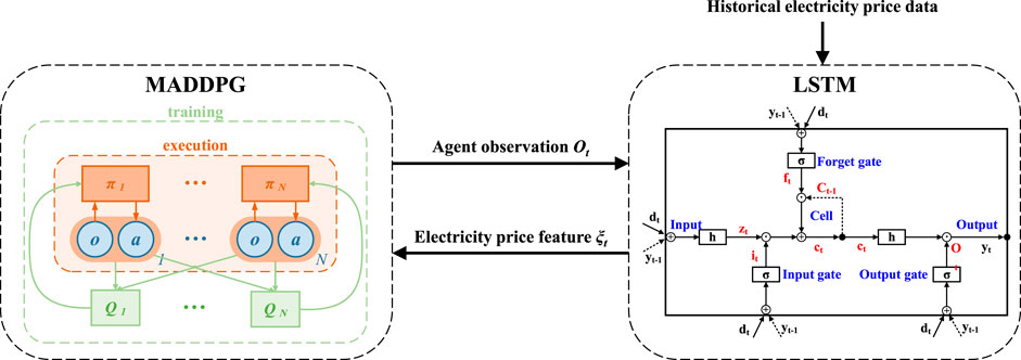
FIGURE 3. Structure of LEMADDPG algorithm.

In the policy network section, the algorithm uses the idea of the deterministic policy gradient (DPG) (Silver et al., 2014): it changes from outputting the probability distribution of actions to directly outputting specific actions and updates the network parameters by maximizing the expected cumulative reward of each agent. This is conducive to the agent’s learning in continuous action spaces. The agent first obtains its own observed information o from the environment. Then, it chooses and outputs the current action a according to the current policy π in its own policy network. Notably, the agent uses only its own local information for observation and execution, without needing to know the global state information. After the agent obtains the current observation o_i,t in the environment, it selects the current action a_i,t through the policy network μ_i to provide its own current policy selection. Meanwhile, to improve the degree of exploration of the agent during training in a specific environment, a white noise signal N_t is added each time the policy network outputs an action, that is

$a_{i,t}={\mu }_i\left(o_{i,t}\right)+N_t(23)$

In the value network section, to solve the non-stationarity problem in the multi-agent environment, the algorithm uses a centralized method to evaluate the policy of each agent. When each agent’s value network Critic evaluates the policy value Q, it not only uses its own Actor information but also considers the information of all agents. In other words, the Critic of each agent is centralized. This is key to implementing centralized training and distributed execution.

The LEMADDPG algorithm uses the experience replay (Mnih et al., 2013) strategy to enhance the stability of the learning process. The experience replay method stores the interaction data of each agent in the environment in a shared replay buffer. During training, a batch of data is randomly sampled for repetitive learning, significantly increasing the learning efficiency of the algorithm. The specific method is as follows: Each time the agent’s policy network generates action a_i,t based on the current observation o_i,t, the environment returns the current reward value r_i and the observation at the next moment o_i,t+1 based on the action. At this point, all related information set {o_1,t, o_2,t, …, o_N,t, a_1,t, …, a_N,t, r₁, …, r_i, o_1,t+1, …, o_i,t+1} is stored in the experience replay pool $\mathcal{D}$, waiting to be used as training samples for the neural network. Following this, the system undergoes a state transition.

The target network strategy refers to each agent maintaining a target network that has the same structure as its current network but updates parameters more slowly. The target network is used to calculate the approximation of the expected cumulative reward, thereby reducing the oscillation of the target function and accelerating the convergence speed of the algorithm, as shown in Figure 4. Similar to the original network, the target network contains policy and value networks. The parameters at initialization use the policy network parameters and value network parameters from the original network, but their update methods differ substantially.

FIGURE 4

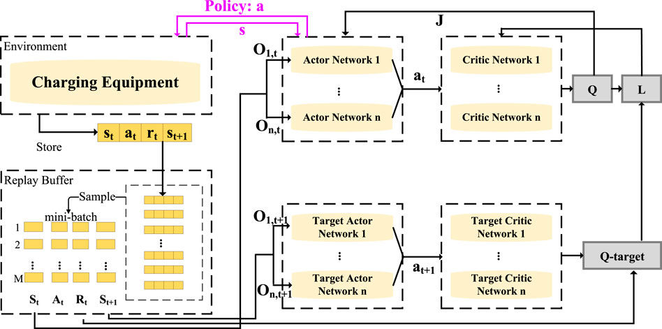
FIGURE 4. Network structure and training process of MADDPG.

The objective of training the original network is to maximize the expected reward of its policy network while minimizing the loss function of the value network (Dai et al., 2021). The specific update procedures are as follows:

The update formula for the policy network is:

${\nabla }_{{\theta }_i}J\left({\mu }_i\right)=E_{x,a\sim \mathcal{D}}\left[{\nabla }_{{\theta }_i}{\mu }_i\left(a_i|o_i\right){\nabla }_{a_i}{Q}_i^{\mu }\left(x,a_1,\dots ,a_N\right){|}_{a_i={\mu }_i\left(o_i\right)}\right](24)$

where ${\nabla }_{{\theta }_i}J({\mu }_i)$ is the gradient of the expected reward of the policy network with network parameters θ_i. ${\nabla }_{a_i}{Q}_i^{\mu }(x,a_1,\dots ,a_N)$ is the gradient of the action value function output by the network under the current state x and joint action a_t = {a₁, a₂, …, a_N} with respect to the action. ${\nabla }_{{\theta }_i}{\mu }_i(a_i|o_i)$ is the gradient of the action output of the policy network with respect to network parameter θ_i.

The update formula for the value network is:

$L\left({\theta }_i\right)=E_{x,a,r,x^{\prime }}\left[{\left(Q_i^{\mu }\left(x,a_1,\dots ,a_N\right)-y\right)}^2\right](25)$

where L(θ_i) is the loss function of the value network. y is the actual action value function, which can be represented as:

$y=r+\gamma Q_i^{{\mu }^{\prime }}\left(x^{\prime },{a_1}^{\prime },\dots ,a_N^{\prime }\right){|}_{{a^{\prime }}_j={{\mu }^{\prime }}_j\left(o_j\right)}(26)$

where γ is the discount factor, 0 ≤ γ < 1. $Q_i^{{\mu }^{\prime }}(x^{\prime },{a_1}^{\prime },\dots ,a_N^{\prime })$ is the action value function of the target network.

After a complete round of learning, we use α as the update step size to update the parameters of the original network, which can be expressed as:

$\begin{array}{c}{\theta }_i\leftarrow {\theta }_i+\alpha \cdot {\nabla }_{{\theta }_i}J\left({\mu }_i\right),\hfill \\ {\theta }_i\leftarrow {\theta }_i-\alpha \cdot {\nabla }_{{\theta }_i}L\left({\theta }_i\right)\hfill \end{array}(27)$

The target network uses a soft update method to update the network parameters. It assigns a weight τ (0 ≤ τ < 1) to the parameters about to be updated, preserving a portion of the original parameters. This results in smaller changes in the target network’s parameters and smoother updates, which can be expressed as:

${{\theta }_i}^{\prime }\leftarrow \tau {\theta }_i+\left(1-\tau \right){{\theta }_i}^{\prime }(28)$

4.3 Algorithm overflow

The structure of the LEMADDPG algorithm is shown in Figure 3. The specific flow is shown in Algorithm 1. The system first initializes the EV charging and discharging environment according to the set parameters and then generates the initial observation O₀. For each EV agent, it selects the action a_i,t according to its current observation o_i,t and strategy. Then, the joint action a_t is performed, each agent obtains its own reward r_i,t from the environment and obtains the observation o_i,t+1 of the next stage. The system records all information $\left(O_t,a_t,r_t,O_{t+1}\right)$ at this time and stores the quadruple in the experience replay pool $\mathcal{D}$. Then, the current system observation O_t is input into the LSTM network, and the electricity price feature ξ_t output under the current state is obtained. The current time electricity price feature ξ_t replaces the real electricity price λ_t for state update, that is:

$o_{i,t}=\left\{{\lambda }_t,u_{i,t},SO{C}_{i,t}\right\}\to o_{i,t}^{\prime }=\left\{{\xi }_t,u_{i,t},SO{C}_{i,t}\right\}(29)$

Next, the system state is transferred. If the experience replay pool $\mathcal{D}$ is full, random sampling is performed for the agent to learn from experience. The agent uses the minimization loss function to update its Critic network and the gradient policy to update its Actor network. Then, all target network parameters are updated using a soft update method. At this point, a round of training is over, and the system returns to the initial state to start the next round of training.

ALGORITHM 1

Algorithm 1. LEMADDPG algorithm.

5 Experimental results

5.1 Environment setup

We consider a smart community with a total of N EVs, and we simulate the process of the fleet plugging into the charging device over a 24-h period, from 0:00 on 1 day to 0:00 the next day, totaling 24 time periods. The relevant parameters of the vehicle are shown in Table 1. The parameters of the EV charging and discharging model are shown in Table 2.

TABLE 1

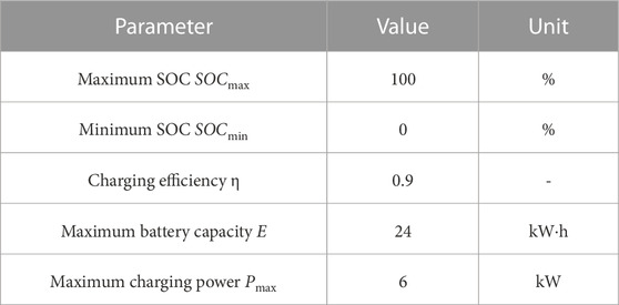
TABLE 1. EV related parameters.

TABLE 2

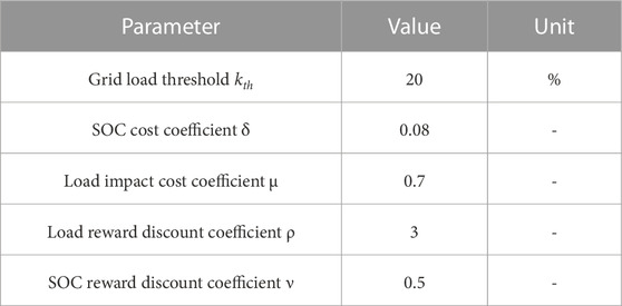
TABLE 2. EV charging and discharging model parameters.

The training process uses TOU electricity price data provided by a power company in a city in the UK. We select the electricity prices from April 2019 as the training dataset and electricity prices from September 2020 as the validation dataset. The TOU electricity price data is shown in Figure 5.

FIGURE 5

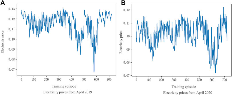
FIGURE 5. The TOU electricity prices of a city in the UK: (A) Electricity price from April 2019; (B) Electricity price from April 2020.

5.2 MADDPG results analysis

Upon initialization of the environment, we use the Monte Carlo method to simulate and generate the relevant initial variables for each EV. This includes the initial SOC, the desired SOC, and the times when the EV arrives at and leaves the charging station. The initial system observation includes the relevant states of all EVs, which can be represented by a 4N-dimensional vector $O_0=\left\{SO{C}_{\mathrm{1,0}},SO{C}_{\mathrm{2,0}},\dots ,SO{C}_{N,0},SO{C}_{1,\mathrm{i}\mathrm{d}\mathrm{e}\mathrm{a}\mathrm{l}},\dots ,SO{C}_{N,\mathrm{i}\mathrm{d}\mathrm{e}\mathrm{a}\mathrm{l}},T_1^{\text{start}},\dots T_N^{\text{start}},\right.\left.T_1^{\text{end}},\dots T_N^{\text{end}}\right\}$. The algorithm first starts from the initial state and advances according to the scheduling step size. Each agent in the EV cluster sequentially selects charging or discharging actions under its current policy and then receives rewards from the environment. Then, the EV cluster carries out all actions and receives observations for the next period from the environment. The related data are stored in the experience replay pool, and the environment state transitions until the maximum number of scheduling steps is reached or the total reward of all agents in the system reaches a steady state.

To study the effectiveness of the MADDPG algorithm for the EV charging and discharging optimization scheduling problem, we first use the traditional MADDPG algorithm to run this case. The algorithm parameter settings are shown in Table 3.

TABLE 3

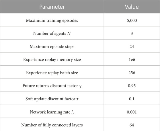
TABLE 3. MADDPG algorithm parameters.

The total reward curve of the MADDPG-based EV cluster’s charging and discharging is shown in Figure 6, with the following analysis.

FIGURE 6

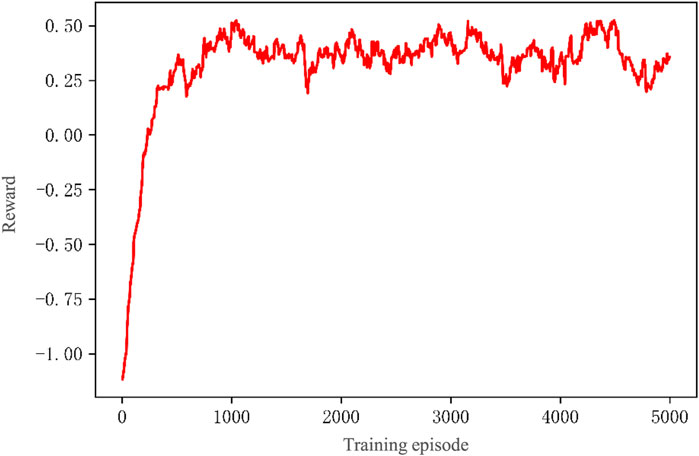
FIGURE 6. Total reward curve of the MADDPG algorithm.

(1) The horizontal axis represents the training round. The vertical axis represents the total reward obtained by the EV agent cluster in the corresponding round. For easy observation, the data have been smoothed with a smoothing factor of 0.95.

(2) The total number of training episodes is 5,000. The experiment runs for 30 min under the given conditions. As shown in the figure, the total reward curve rises rapidly in the initial 800 rounds, after which the reward curve gradually becomes smooth and converges. Finally, it stabilizes around 0.42, indicating that the algorithm has converged.

The converged MADDPG algorithm is validated on the TOU electricity price dataset for September 2020. For ease of observation, we extract the change in TOU electricity price and the corresponding action curve of the EV agents within 50 scheduling steps for comparison. Figure 7 shows the charging and discharging schemes of a certain EV following the TOU electricity price. The analysis is as follows.

FIGURE 7

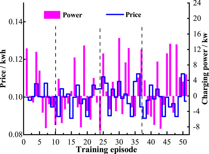
FIGURE 7. Charging and discharging schemes of a certain EV following the TOU electricity price.

(1) The blue curve represents the time-of-use electricity price, the purple curve represents the charging and discharging power of the EV, and the black dashed line marks the observation points.

(2) At each observation point, the agent chooses to charge at a higher power when the electricity price is at a low point and chooses to charge at a lower power when the electricity price is at a peak. This indicates that the converged algorithm can timely adjust the charging and discharging power based on changes in the TOU electricity price.

(3) The Kendall correlation coefficient between the TOU electricity price and the charging and discharging actions of the agent is −0.245. Since the electricity price is one of the factors affecting the charging and discharging of EVs, the two do not show a strong negative correlation but a weak negative correlation. However, this still indicates that to some extent, the agent can follow the changes in electricity prices and make corresponding actions, i.e., tending to reduce charging power when the price is high and increase power when the price is low. This is consistent with the expected results of the experiment.

5.3 LEMADDPG results analysis

To fully utilize the historical data of TOU electricity prices, this paper adopts an LSTM network to extract the temporal features of electricity prices to guide the agent in decision making. We choose the TOU electricity price data from April 2019 as the input for LSTM training, with the output being a price series with temporal features. The learning rate is set to 0.01. Figure 8 shows the results after 2000 rounds of LSTM training. The blue curve in the figure represents the original electricity prices, and the orange curve represents the prices predicted by the LSTM using temporal features. The results indicate that LSTM can extract the features of time-of-use electricity price data and make reasonable predictions for future prices.

FIGURE 8

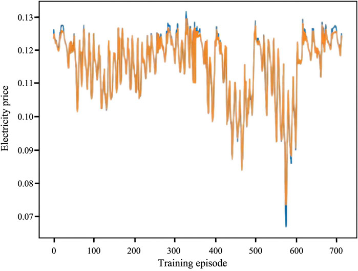
FIGURE 8. Electricity prices predicted by the LSTM network.

During the model training process, we replace the real electricity price information with the electricity price features extracted by the LSTM when updating the system state observation. The total reward curve for charging and discharging of the EV cluster based on the LEMADDPG algorithm is shown in Figure 9, with the following analysis.

FIGURE 9

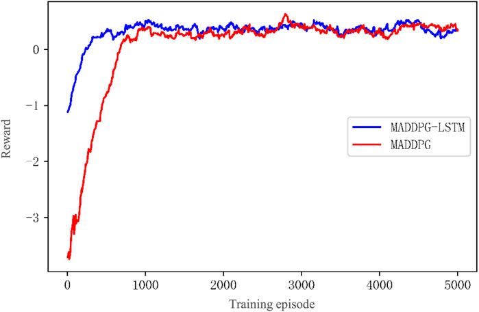
FIGURE 9. Total reward curves of MADDPG before and after the adding LSTM.

(1) The horizontal axis is the number of training rounds. The vertical axis is the total reward obtained by the EV agent cluster in the corresponding round. For ease of observation, the data have been smoothed with a smoothing factor of 0.95.

(2) The total number of training episodes is 5,000. The red curve represents the total reward change of the original MADDPG algorithm. The blue curve represents the total reward change of the MADDPG algorithm after adding the LSTM. Both curves show a rapid rise for the first 600 rounds. After 600 rounds, the reward curve of LEMADDPG has converged, while the reward curve of MADDPG begins to flatten after 800 rounds. After repeating the experiment five times, it can be calculated that the average convergence speed of the improved MADDPG algorithm has increased by 19.72% compared to that of the original MADDPG. After 1,000 rounds, the total rewards of both eventually stabilize around 0.42.

(3) The initial state of the system differs due to the substitution of the input electricity price information with the temporal features extracted by LSTM, resulting in a distinct difference in the initial segments of the two curves.

(4) The above results show that after adding the LSTM network in MADDPG, there is almost no change in the stable value of the total reward after convergence. However, the convergence speed of the algorithm has significantly improved.

5.4 Comparative experiment

To validate the adaptability and superiority of the proposed LEMADDPG algorithm, we conducted two comparative experiments, one involving the performance comparison of different algorithms under the same scale of EVs, and the other involving different algorithms under varying scales of EVs. The parameter settings of the algorithms are the same as those in Table 3.

Figure 10 shows the comparative results of comprehensive costs under the same scale of EVs. The comprehensive cost is calculated as the cumulative value every 24 h. The results indicate that the comprehensive cost of the policy obtained by LEMADDPG is the lowest, at 2.94, which is 2.97% lower than the cost of DDPG, and 6.67% lower than the cost of DQN. The total reward with 3 EVs of the LEMADDPG, DDPG, and DQN algorithms are shown in Table 4. In terms of the speed of reward convergence, compared to LEMADDPG, the benchmark algorithms DQN and DDPG converge even faster at 120 and 500 rounds, respectively. This is because the LEMADDPG algorithm is more complex and its advantages are not obvious when addressing small-scale decision problems. In terms of the steady-state value of the reward, the policy obtained by LEMADDPG achieves higher reward values, converging to 0.42. The above results show that the LEMADDPG algorithm has the best steady-state reward value and a fast response speed.

FIGURE 10

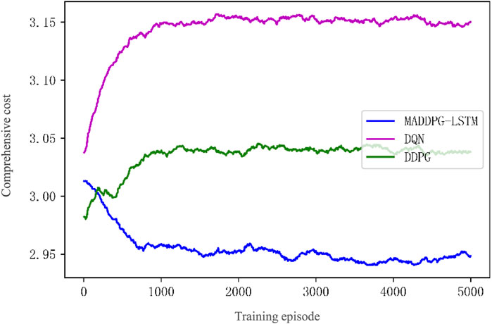
FIGURE 10. Composite cost curves of three algorithms.

TABLE 4

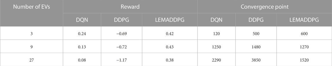
TABLE 4. Comparison of rewards and convergence points under different scales of EVs.

Table 4 shows the training comparison results for different algorithms with EV quantities of 3, 9, and 27, respectively. It can be observed that compared to the two benchmark algorithms, LEMADDPG has achieved higher convergence reward values with all three scales. This indicates that LEMADDPG can seek better charging and discharging strategies for different scales of EVs. As for convergence speed, larger scales require more resources for the algorithm to find the optimal strategy, leading to a delay in the convergence points for all three algorithms as the scale of EVs increases. However, it can be observed that due to its simple structure, DQN has the fastest convergence speed in scenarios with 3 and 9 EVs, converging in 120 and 1,250 episodes respectively. However, as the number of EVs grows exponentially, the LEMADDPG algorithm demonstrates a clear advantage. When managing 27 EVs, the convergence speed of the LEMADDPG algorithm is 33% faster than DQN. This indicates that the algorithm proposed in this paper is capable of addressing the charging management problem of a large number of EVs.

5.5 Impact of parameters

The MADDPG algorithm is highly sensitive to network parameters. This section focuses on some parameters in MADDPG, demonstrating and comparing the impact of different parameters on the performance of the algorithm.

5.5.1 Soft update frequency

The frequency of soft updates is primarily controlled by the soft update discount factor τ. The smaller the τ value is, the less the target network parameters change, and the more stable the algorithm will be. However, the convergence speed will also be slower. Conversely, the larger the τ value is, the faster the network parameters change, and the algorithm can accelerate convergence. However, it may become unstable during the training process more easily. Therefore, to balance the convergence speed and stability of the algorithm, an appropriate τ value should be chosen. Figure 11 shows the total reward variation curves of the LEMADDPG algorithm with τ = 0.01 and τ = 0.1, respectively, with the following analysis.

FIGURE 11

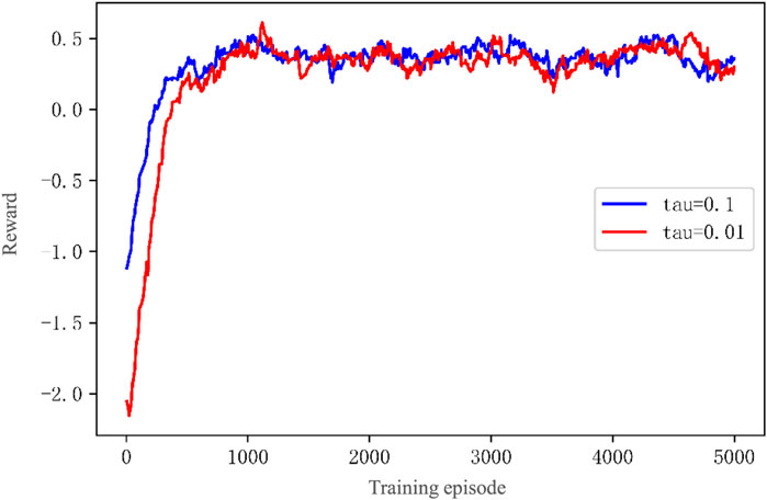
FIGURE 11. LEMADDPG Total Reward Curves with Different Soft Update Discount Factors τ.

(1) The total reward curve for τ = 0.1 gradually stabilizes after 600 rounds, while the total reward curve for τ = 0.01 tends to converge around 500 rounds.

(2) After 2000 episodes, both have converged to fluctuate within a certain area. There is no significant difference in the steady-state values of the total rewards.

(3) The above results indicate that, assuming steady-state convergence is assured, choosing τ = 0.01 can accelerate the convergence of the algorithm without significantly affecting the steady-state value of the total reward.

5.5.2 Learning rate

The learning rate l_r represents the update speed of the neural network’s own strategy. If l_r is too small, the network tends to converge slowly. If l_r is too large, the network loss will exacerbate oscillation or even result in divergence. Therefore, an appropriate network learning rate must be selected to ensure that the network can converge quickly. Figure 12 shows the total reward variation curves of the LEMADDPG algorithm with l_r = 0.001 and l_r = 0.01. The analysis is as follows.

FIGURE 12

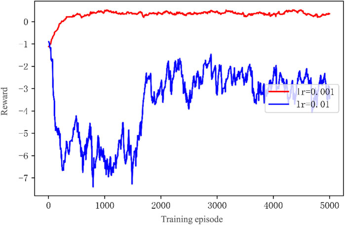
FIGURE 12. LEMADDPG Total Reward Curves with Different Learning Rates l_r.

(1) The reward curve of l_r = 0.001 is close to a logarithmic function. Overall, it shows a steady rise and eventually tends to converge. The reward curve of l_r = 0.01 has significant fluctuations, and it diverges in the first 1500 episodes. After 1500 episodes, it starts to rise. It eventually tends to converge near 2000 episodes, but the fluctuations are still large.

(2) In terms of the steady-state value of the total reward, the curve of l_r = 0.01 eventually tends to −2.84. The curve of l_r = 0.001 tends to 0.42.

(3) The above results show that choosing l_r = 0.001 is more beneficial to obtain a stable and higher total reward network. Increasing the learning rate has a clear negative impact on the network, which reduces the steady-state value of the total reward and makes the algorithm unstable.

5.5.3 Expected return rate

To reflect the continuity of decisions, we hope that the policy network of EV agents can consider not only the current action’s income but also the income of several steps after executing the action based on the current observation when selecting actions. That is, we expect agents to perceive the future situation to a certain extent. When the policy network of the agent outputs actions that are given high-value scores by the evaluation network, we use the long-term return discount factor γ to express the consideration degree of the evaluation network for the future. The larger the γ, the more the agent can consider future returns. An excessively small γ will make the evaluation network unable to foresee future events in time, leading to a slower update speed of the policy network. By contrast, an excessively large γ will lead to low prediction accuracy of the future of the agent’s evaluation network, making its prediction results less credible, thereby making the policy network’s updates more frequent, slowing the convergence speed and even causing the algorithm to diverge.

In the problem of optimizing the charging and discharging scheduling of EVs, we hope that the agent can consider future factors such as electricity price changes and environmental information changes to a certain extent. Therefore, it is necessary to select an appropriate return discount factor γ. Figure 13 shows the total reward variation curves of the LEMADDPG algorithm with γ = 0.9 and γ = 0.99. The analysis is as follows:

FIGURE 13

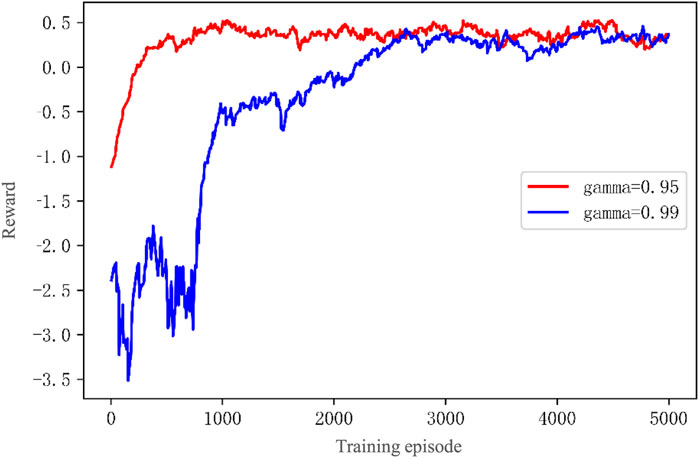
FIGURE 13. LEMADDPG Total Reward Curves with Different Long-term Return Discount Factors γ.

(1) The curve of γ = 0.9 tends to converge near 800 episodes, while the curve of γ = 0.99 gradually becomes stable and converges after 1100 episodes.

(2) After 2800 episodes, both have converged. The steady-state value of the γ = 0.9 curve is 0.42, and the steady-state value of the γ = 0.99 curve is 0.38.

(3) The above results show that choosing a lower long-term return discount factor γ = 0.9 is beneficial to algorithm training. If the discount factor is too large, the agent is significantly influenced by future factors when making decisions and cannot find an appropriate improvement direction in the initial exploration stage, leading to relatively slow convergence of the algorithm.

6 Conclusion

Aiming at solving the optimization scheduling problem of EV charging and discharging in the smart grid, this paper establishes a grid model involving the grid, charging equipment, and EVs. In this model, EVs can conduct real-time bidirectional communication with the grid through the charging device, exchanging current TOU electricity prices and state information of the EVs. By taking into account factors such as charging and discharging costs, user demands, and grid stability, the model aims to minimize the comprehensive cost during the charging and discharging process. This paper enhances the MADDPG algorithm with LSTM network, which is used to extract time series features from historical electricity price data, thereby guiding the charging and discharging strategies of the agents. The simulation results demonstrate that, the proposed method LEMADDPG algorithm improves the training convergence speed by 19.72% compared to the MADDPG algorithm. More critically, when addressing charging issues of EVs of various scales, the proposed method shows the obvious advantages in formulating strategies for large-scale EVs. Compared to DQN, it converges 33% faster and achieves a superior policy optimization.

Our combined LSTM and MADDPG method demonstrates potential, yet faces challenges in data dependency and interpretability. While we’ve ensured robust training in data-rich environments, practical applications may require strategies like transfer learning. Moreover, addressing model transparency remains a priority, and our future study will explore integrating explainable AI techniques to enhance model clarity and interpretability, aiming to make our contributions even more valuable to the broader scientific community.

Data availability statement

The original contributions presented in the study are included in the article/Supplementary material, further inquiries can be directed to the corresponding author.

Author contributions

DA: Conceptualization, Formal analysis, Investigation, Funding acquisition. FC: Methodology, Writing–review and editing, Validation. XK: Data curation, Writing–original draft.

Funding

The author(s) declare financial support was received for the research, authorship, and/or publication of this article. This work was supported in part by the National Natural Science Foundation of China under Grant 62173268; in part by the Major Research Plan of the National Natural Science Foundation of China under Grant 61833015.

Conflict of interest

The authors declare that the research was conducted in the absence of any commercial or financial relationships that could be construed as a potential conflict of interest.

Publisher’s note

All claims expressed in this article are solely those of the authors and do not necessarily represent those of their affiliated organizations, or those of the publisher, the editors and the reviewers. Any product that may be evaluated in this article, or claim that may be made by its manufacturer, is not guaranteed or endorsed by the publisher.

References

Chen, N., Sun, X., and Ma, Z. (2021). The impact of electric vehicles connected to the grid on grid harmonics. Electron. Test. 17, 122–123. doi:10.16520/j.cnki.1000-8519.2021.17.043

CrossRef Full Text | Google Scholar

Chen, Y., Wang, W., and Yang, Y. (2023). Power grid dispatching optimization based on electric vehicle charging load demand prediction. Electeic Eng. 5, 31–33. doi:10.19768/j.cnki.dgjs.2023.05.008

CrossRef Full Text | Google Scholar

Dai, W., Liu, A., Shen, X., Ma, H., and Zhang, H. (2021). Online optimization of charging and discharging behavior of household electric vehicle cluster based on maddpg algorithm. J. Northeast Electr. Power Univ. 41, 80–89. doi:10.19718/j.issn.1005-2992.2021-05-0080-10

CrossRef Full Text | Google Scholar

Ding, T., Zeng, Z., Bai, J., Qin, B., Yang, Y., and Shahidehpour, M. (2020). Optimal electric vehicle charging strategy with markov decision process and reinforcement learning technique. IEEE Trans. Industry Appl. 56, 5811–5823. doi:10.1109/tia.2020.2990096

CrossRef Full Text | Google Scholar

He, Y., Yang, X., Chen, Q., Bu, S., Xu, Z., Xiao, T., et al. (2021). Review of intelligent charging and discharging control and application of electric vehicles. Power Gener. Technol. 42, 180–187. doi:10.3760/cma.j.cn112152-20190322-00182

CrossRef Full Text | Google Scholar

Jin, J., and Xu, Y. (2020). Optimal policy characterization enhanced actor-critic approach for electric vehicle charging scheduling in a power distribution network. IEEE Trans. Smart Grid 12, 1416–1428. doi:10.1109/tsg.2020.3028470

CrossRef Full Text | Google Scholar

Kim, I.-S. (2008). Nonlinear state of charge estimator for hybrid electric vehicle battery. IEEE Trans. Power Electron. 23, 2027–2034. doi:10.1109/tpel.2008.924629

CrossRef Full Text | Google Scholar

Konda, V., and Tsitsiklis, J. (1999). “Actor-critic algorithms,” in Advances in neural information processing systems 12. Editors S. A. Solla, and T. K. Leen (Cambridge: MIT Press).

Google Scholar

Liao, X., Li, J., Xu, J., and Song, C. (2021). Research on coordinated charging control for electric vehicles based on mdp and incentive demand response. J. Electr. Power Sci. Technol. 36, 79–86. doi:10.19781/j.issn.1673-9140.2021.05.010

CrossRef Full Text | Google Scholar

Liu, J., Guo, H., Xiong, J., Kato, N., Zhang, J., and Zhang, Y. (2019). Smart and resilient ev charging in sdn-enhanced vehicular edge computing networks. IEEE J. Sel. Areas Commun. 38, 217–228. doi:10.1109/jsac.2019.2951966

CrossRef Full Text | Google Scholar

Liu, Y., Deng, B., Wang, J., Yu, Y., and Chen, D. (2022). Charging scheduling strategy of electric vehicle based on multi-objective optimization model. J. Shenyang Univ. Technol. 44, 127–132. doi:10.7688/j.issn.1000-1646.2022.02.02

CrossRef Full Text | Google Scholar

Loisy, A., and Heinonen, R. A. (2023). Deep reinforcement learning for the olfactory search pomdp: a quantitative benchmark. Eur. Phys. J. E 46, 17. doi:10.1140/epje/s10189-023-00277-8

PubMed Abstract | CrossRef Full Text | Google Scholar

Long, T., Ma, X.-T., and Jia, Q.-S. (2019). “Bi-level proximal policy optimization for stochastic coordination of ev charging load with uncertain wind power,” in 2019 IEEE Conference on Control Technology and Applications (CCTA), Hong Kong, China, 19-21 August 2019, 302–307.

CrossRef Full Text | Google Scholar

Lowe, R., Wu, Y. I., Tamar, A., Harb, J., Pieter Abbeel, O., and Mordatch, I. (2017). “Multi-agent actor-critic for mixed cooperative-competitive environments,” in Advances in Neural Information Processing Systems 30: Annual Conference on Neural Information Processing Systems 2017, Long Beach, CA, USA, December 4-9, 2017.

Google Scholar

Lu, S., Ying, L., Wang, X., and Li, W. (2020). Charging load prediction and optimized scheduling of electric vehicle quick charging station according to user travel simulation. Electr. Power Constr. 41, 38–48. doi:10.12204/j.issn.1000-7229.2020.11.004

CrossRef Full Text | Google Scholar

Mnih, V., Kavukcuoglu, K., Silver, D., Graves, A., Antonoglou, I., Wierstra, D., et al. (2013). Playing atari with deep reinforcement learning. arXiv preprint arXiv:1312.5602.

Google Scholar

Nachum, O., Norouzi, M., Xu, K., and Schuurmans, D. (2017). “Bridging the gap between value and policy based reinforcement learning,” in Advances in Neural Information Processing Systems 30: Annual Conference on Neural Information Processing Systems 2017, Long Beach, CA, USA, December 4-9, 2017.

Google Scholar

Pan, Z., Yu, T., Chen, L., Yang, B., Wang, B., and Guo, W. (2020). Real-time stochastic optimal scheduling of large-scale electric vehicles: a multidimensional approximate dynamic programming approach. Int. J. Electr. Power & Energy Syst. 116, 105542. doi:10.1016/j.ijepes.2019.105542

CrossRef Full Text | Google Scholar

Rawat, T., Niazi, K. R., Gupta, N., and Sharma, S. (2019). Impact assessment of electric vehicle charging/discharging strategies on the operation management of grid accessible and remote microgrids. Int. J. Energy Res. 43, 9034–9048. doi:10.1002/er.4882

CrossRef Full Text | Google Scholar

Shao, S., Pipattanasomporn, M., and Rahman, S. (2011). Demand response as a load shaping tool in an intelligent grid with electric vehicles. IEEE Trans. Smart Grid 2, 624–631. doi:10.1109/tsg.2011.2164583

CrossRef Full Text | Google Scholar

Shi, J., Gao, Y., Wang, W., Yu, N., and Ioannou, P. A. (2019). Operating electric vehicle fleet for ride-hailing services with reinforcement learning. IEEE Trans. Intelligent Transp. Syst. 21, 4822–4834. doi:10.1109/tits.2019.2947408

CrossRef Full Text | Google Scholar

Shi, X., Chen, Z., Wang, H., Yeung, D.-Y., Wong, W.-K., and Woo, W.-c. (2015). “Convolutional lstm network: a machine learning approach for precipitation nowcasting,” in Advances in Neural Information Processing Systems 28: Annual Conference on Neural Information Processing Systems 2015, Montreal, Quebec, Canada, December 7-12, 2015.

Google Scholar

Silver, D., Lever, G., Heess, N., Degris, T., Wierstra, D., and Riedmiller, M. (2014). “Deterministic policy gradient algorithms,” in Proceedings of the 31 st International Conference on Machine Learning, Beijing, China, 22-24 June 2014, 387–395.

Google Scholar

Vandael, S., Claessens, B., Ernst, D., Holvoet, T., and Deconinck, G. (2015). Reinforcement learning of heuristic ev fleet charging in a day-ahead electricity market. IEEE Trans. Smart Grid 6, 1795–1805. doi:10.1109/tsg.2015.2393059

CrossRef Full Text | Google Scholar

Wan, Z., Li, H., He, H., and Prokhorov, D. (2018). Model-free real-time ev charging scheduling based on deep reinforcement learning. IEEE Trans. Smart Grid 10, 5246–5257. doi:10.1109/tsg.2018.2879572

CrossRef Full Text | Google Scholar

Wen, Z., O’Neill, D., and Maei, H. (2015). Optimal demand response using device-based reinforcement learning. IEEE Trans. Smart Grid 6, 2312–2324. doi:10.1109/tsg.2015.2396993

CrossRef Full Text | Google Scholar

Wu, T., Zhou, P., Liu, K., Yuan, Y., Wang, X., Huang, H., et al. (2020). Multi-agent deep reinforcement learning for urban traffic light control in vehicular networks. IEEE Trans. Veh. Technol. 69, 8243–8256. doi:10.1109/tvt.2020.2997896

CrossRef Full Text | Google Scholar

Xiong, L., Mao, S., Tang, Y., Meng, K., Dong, Z., and Qian, F. (2021). Reinforcement learning based integrated energy system management: a survey. Acta Autom. Sin. 47, 2321–2340. doi:10.16383/j.aas.c210166

CrossRef Full Text | Google Scholar

Zhang, Y., Rao, X., Zhou, S., and Zhou, Y. (2022). Research progress of electric vehicle charging scheduling algorithmsbased on deep reinforcement learning. Power Syst. Prot. Control 50, 179–187. doi:10.19783/j.cnki.pspc.211454

CrossRef Full Text | Google Scholar

Zhao, J., Wen, F., Yang, A., and Xin, J. (2011). Impacts of electric vehicles on power systems as well as the associated dispatching and control problem. Automation Electr. Power Syst. 35, 2–10. doi:10.1111/j.1365-2761.2010.01212.x

CrossRef Full Text | Google Scholar

Zhao, X., and Hu, J. (2021). Deep reinforcement learning based optimization for charging of aggregated electric vehicles. Power Syst. Technol. 45, 2319–2327. doi:10.13335/j.1000-3673.pst.2020.1418

CrossRef Full Text | Google Scholar