Large-eddy simulation of the effects of horizontal and vertical adjustments in a wind farm

1 Introduction

Wind power, as a very promising clean and sustainable energy form, has shown rapid development during the recent decades. In particular, in Europe, large wind energy penetration has already been achieved with an ever-increasing contribution to total energy production (Kuik et al., 2016). Under the major national strategic goals of achieving carbon peak and carbon neutralization in China, the new electric power system of our country is transforming mainly from coal to new energy. According to the 14th Five-Year Plan, 170 million kW of wind power is expected to be installed in western and northern China by 2025 (Liu and Zhang, 2020; Qin, 2021; Wang, 2021).

Wind turbines absorb wind energy through impeller rotation, resulting in a downwind wind speed decrease, which is known as the “wake effect” (Göçmen et al., 2016). If the downstream turbines were in the wake of the upstream turbines, the downstream turbines’ power generation and, thus, the total power generation of the whole wind power farm would be significantly reduced (Li et al., 2020; Verma et al., 2021; Verma et al., 2022). Previous studies have pointed out that in wind farms currently put into operation, the wake effect can reduce the power generation of wind farms by 15%–50% (Smith et al., 2006; Barber et al., 2011). Under the limited area and cost, reducing the impact of wake to the furthest possible extent is one of the important goals for the sustainable development of wind power. In order to reduce the impact of wakes and to maximize the efficiency of wind power generation, many findings have stated that different wind farm layouts cause varying wind output generation, and advanced wind farm layouts limit wake effects and ensure good wind farm performance (Cal et al., 2010; Calaf et al., 2010; Yang et al., 2012; Archer et al., 2013; Meyers and Meneveau, 2013; Stevens and Meneveau, 2020). The findings, as mentioned so far, have undoubtedly made an important contribution to the construction of more performance-efficient wind farms. The horizontal variations in the wind farm layout have been studied extensively, while considering the horizontal staggering and vertical staggering together to limit the wake effects in large wind farms has been relatively unexplored. Meanwhile, to study the origin and characteristics of wake meandering and computational models, the reference data that can be used to verify and improve model calculations, such as an experiment or large-eddy simulation (LES) approach, can perform well (Yang and Sotiropoulos, 2019; Li et al., 2022).

In this work, we adapted the simulated data from LES to identify horizontal and vertical structures of wake effects directly and study the effect of the wind farm layout on the generated wind power of a whole farm yield. The primary aim was to quantify the sensitivity of the wind farm performance to the array layout of horizontal and vertically staggered wind farms in terms of stream-wise and span-wise turbine spacing changes and the interlace degree and the hub height differences between consecutive turbine rows using large-eddy simulation. It starts with a description of the numerical method and simulation setup in section 2. In section 3, an identification of the structures of wake effects in a farm field and an analysis of the power output of horizontal and vertically staggered wind farms are provided. Finally, a summary and the conclusions are presented in Section 4.

2 Methods

2.1 Numerical method

The large-eddy simulation technology is an emerging frontier in resolving the turbulence structure, which has been widely applied in multiple fields, including the atmospheric environment (Ma et al., 2020; Ma et al., 2021; Wang et al., 2023) and wind engineering (Witha et al., 2014). The simulations in this study were performed with the parallelized LES model PALM (Raasch and Schroter, 2001). The PALM model is based on the non-hydrostatic, filtered, incompressible Navier–Stokes equations in the Boussinesq-approximated form (an elastic approximation is available as an option for simulating deep convection). By default, PALM has at least six prognostic quantities: the velocity components u, v, and w on a Cartesian grid; the potential temperature θ; water vapor mixing ratio q_v; and possibly a passive scalar s. Furthermore, an additional equation is solved for either the subgrid-scale turbulent kinetic energy (SGS-TKE, LES mode, default) or the total turbulent kinetic energy. The simulations in this study were performed with a wind turbine model (WTM) included in the parallelized LES model PALM. The WTM contains a wind turbine controller, including speed control, pitch control, and yaw control, which can be switched on and off separately (Storey et al., 2013). The PALM-WTM is based on the common actuator disk model (ADM) approach, in which the rotor of a wind turbine is represented by a permeable disk that extracts energy from the flow by applying a thrust force at the disk (Calaf et al., 2010). The ADM represents the impact of the rotor on the flow as a porous disk that acts as a homogeneous momentum sink with a thrust force F_T acting against the mean flow:

${\mathrm{F}}_{\mathrm{T}}=-\frac{1}{2}{\mathrm{C}}_{\mathrm{T}}\mathrm{A}{\left(\frac{1}{1-\mathrm{\alpha }}{\mathrm{u}}_{\mathrm{r}}\right)}^2,$

where the thrust coefficient is C_T, the rotor area is A, the axial induction factor is $\mathrm{\alpha }$, and the temporally and rotor disk averaged velocity in direction of the mean flow is ${\mathrm{u}}_{\mathrm{r}}$.

2.2 Simulation setup

In this study, a set of regular turbines with a rated power of 5 MW and a rotor radius of 63 m are used in the PALM-WTM to simulate the wind power generation scenario of a wind farm. A series of scenario simulations are designed in this study with the specific settings shown in Table 1. As shown in Figure 1, in our LES, the computational domain along the flow, span, and vertical directions is 12 × 12 × 1 km³ (L_x×L_y×L_z), where the study domain is 8 × 8 × 1 km³ (L_x×L_y×L_z) and the spatial resolution is 20 m, 20 m, and 20 m, respectively. The initial wind field conditions of the simulation are carried out with uniform horizontal winds in the x-direction as the incoming airflow. The wind speed is up to 8 m s^-1, with the exception of case 1, where the incoming wind speed varies within 0–25 m s^-1, to investigate the sensitivity of power generation to prevailing wind speeds. Periodic boundary conditions are used in the simulation in this study. The buffer zone is set so that the wake of the last row of turbines does not affect the first row under the periodic boundary conditions. The buffer zone method used to eliminate the effect of the periodic boundary condition has been used in Ma et al. (2021). In order to explore the potential wake effect of a turbine in the wind farm, the wind power generation with only one single turbine scenario was simulated, as seen in case 1. The power generation simulation of a linear array of wind farms with increasing stream-wise turbine spacing (S_x = 0.5, 1, 2 km) was designed to investigate the effect of spacing on wake effects (cases 2–4). In order to study the influence of horizontally staggered wind farms, the wind farm layout was changed by adjusting the angle θ = arctan (y_offset/S_x) with respect to the incoming flow direction, as shown in Figure 2A, where y_offset indicates the span-wise offset from one turbine row to the next, as seen in cases 5–10 (Stevens et al., 2014). The degree of vertical staggering is dictated by the elevation/abasement dH relative to the averaged hub height H, i.e., 70 m, in this paper, and the height difference between two consecutive turbine rows is 2 dH. The configuration of the vertically staggered wind farm and the corresponding parameters are shown in Figure 2B. The value of dH was changed to investigate the effect of vertically staggered wind farms on the overall output power (case 11–17). The mean inflow remains in the x-direction in all cases.

TABLE 1

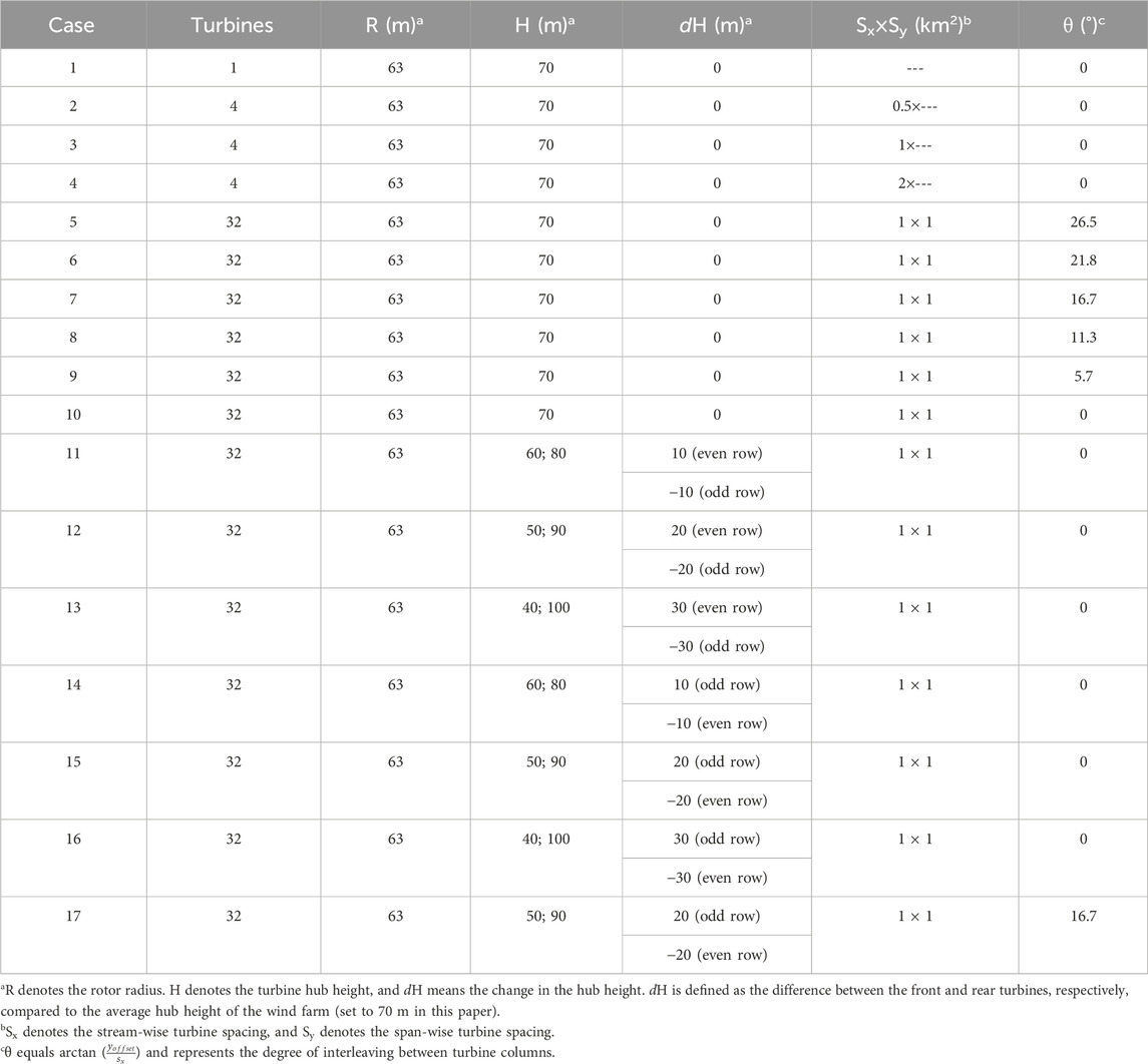
TABLE 1. Wind farm layouts and configurations simulated by PALM-WTM.

FIGURE 1

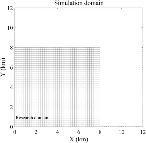
FIGURE 1. Diagram showing the simulation domain in this study.

FIGURE 2

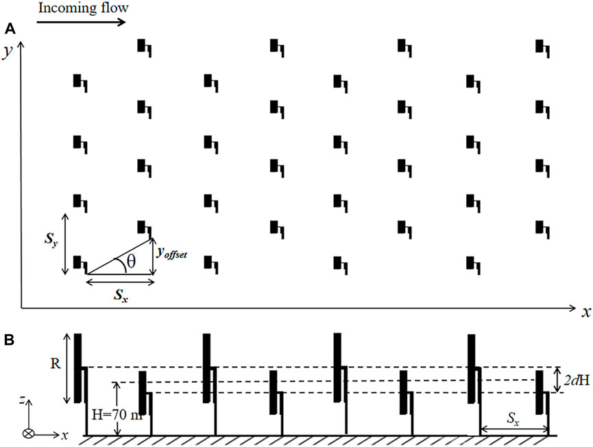
FIGURE 2. Diagram showing the definition of the parameter θ and dH that are used in this study to determine the horizontal and vertical adjustment of the wind farm layout, respectively. (A) Angle θ = arctan (y_offset/S_x) is defined with respect to the incoming flow direction, where y_offset indicates the span-wise offset of subsequent turbine rows, and S_x is the stream-wise distance between the rows. (B) dH is defined as the difference between the front and rear turbines, respectively, compared to the average hub height of the wind farm (set to 70 m in this paper). Therefore, the hub height difference between two consecutive turbine rows is 2 dH.

3 Results and discussion

3.1 Wake effect

As shown in Figure 3A, only one turbine is located at x = 1,000 m and y = 4,000 m in the research domain (8 km × 8 km), of which the simulated wind yield by PALM-WTM is in Figure 3B. At the hub height of 70 m, there are prevailing westerly winds going through the single turbine. The wind speed is uniform (∼7–8 m s^-1) except for the wind passing through the turbine. In the x-direction of y = 4,000 m, a significant weak wind zone with a wind speed of ∼2–3 m s^-1 appears in the range of x = 1 km to x = 3 km. Thus, without any interference, a typical wake generated by an independent turbine is approximately 2 km in length, where the wind speed is about 70% lower than the cut-in wind speed.

FIGURE 3

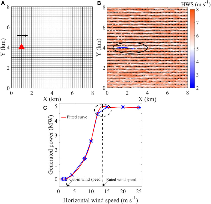
FIGURE 3. Single turbine position in the domain (A); simulated wind field at the height of 70 m (arrow: wind vectors; shaded colors: wind speed) with one turbine (B); determination of the power–wind speed curve from simulated data (C).

In addition to the wake effects, knowing that the power yield of wind farms is directly related to the wind field, we used the LES to further simulate the wind speed dependence. We ran a set of simulations with different horizontal wind speeds (HWS) (1, 2, 4, 8, 10, 12, 15, 20, and 25 m s^-1) at the same hub height to simulate different power generations that can be produced by a single turbine at different wind speeds. Figure 3C presents all the simulation results. It is apparent that with the increase in wind speed, the generated power gradually increases. However, once the wind speed is larger than 15 m s^-1, the generated power maintains the rated power of 5 MW. The power generation increases non-linearly with increasing wind speed. Most prominently, the wind speed that produces the maximum amount of power generation is between 10 and 15 m s^-1. It illustrates that running more cases between 10 and 15 m s^-1 can find the rated wind speed. In order to explain this relationship mathematically, a power–wind speed curve can be determined/fitted from the scatter simulation results. Based on the maximum curvature of the power–wind speed curve, the rated wind speed is determined at 11.4 m s^-1. Without performing more simulations, based on the mathematically fitted curve, we can determine, to some extent, the critical wind speed at which the maximum power is generated. Furthermore, a turbine can generate power once the wind speed exceeds ∼2 m s^-1, which is recognized as the cut-in wind speed.

Figure 4 displays the simulations of horizontal wind speed (HWS) profiles in the y-direction and x-direction, respectively, to assess the horizontal and vertical structures of the wake effect. As depicted by the wind profile in the x–z direction (Figures 4A, C), there is a distinct weak wind zone behind the turbine, approximately 1–2 km in length, with a wind speed of ∼ 4–7 m s^-1. The sharply decreasing wind speed profile extends from the ground to a height of ∼200 m, with a maximum decrease in the wind speed of ∼50%. Further away from the wake in the steam-wise direction (i.e., x = 3 km), the wake effect reduces, with the reduction of wind speed reduced by ∼ 25%. However, in the y–z direction, the wind speed reduction caused by the turbine wake is not as extensive and significant as in the x–z direction (Figures 4B, D). Wind speed reduction contour from the ground level to ∼200 m height does not exceed ∼100 m in length in the span-wise direction. The wind speed decreases to ∼ 4–7 m s^-1, with a maximum decrease of ∼50% compared to the cut-in wind speed. Since the mean inflow in the domain remains in the x-direction, the turbine absorbs wind energy by rotating the impeller, thus creating a wake effect on the airflow in the stream-wise direction. The resulting wind speed disturbance in the y-direction can be extended vertically to the range centered on the hub height of the turbine.

FIGURE 4

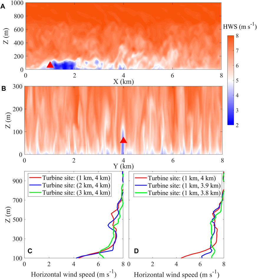
FIGURE 4. Simulated wind profile with one turbine in the stream-wise direction (x) (A); simulated wind profile with one turbine in the span-wise direction (y) (B); vertical wind profiles (C) at (1 km, 4 km), (2 km, 4 km), and (3 km, 4 km), respectively; vertical wind profiles (D) at (1 km, 4 km), (1 km, 3.9 km), and (1 km, 3.8 km), respectively.

3.2 Sensitivity of power yield to turbine spacing

Figure 5 shows the wind field simulation results of three sets of cases (varying turbine spacing of 0.5 km, 1 km, and 2 km, respectively) of four linearly aligned turbines. The horizontal distribution of the wind field above is at the elevation of the hub height. When the turbine spacing is 0.5 km, the wakes produced by the four linearly aligned turbines were almost completely integrated into one wake. The length of the “joint wake” was approximately 2 km in the stream-wise direction, equivalent to the wake length of a single turbine, as identified in Section 3.1. As the distance between the four turbines is 0.5 km, the last three turbines are located exactly in the wake of the first upwind turbine. Therefore, the wake length in the airflow direction of the four turbines is equivalent to that of the first turbine downwind but with a greater intensity of impact. The reduction in wind speeds is more pronounced in the “joint-wake” compared to the wake effect of the individual turbines. The wake effect affected up to 300 m vertically, and the wind speed can be reduced by up to ∼37% (Figure 4; Figure 5C). As the turbine spacing increased to 1 km, there was a wake interference among the wakes produced by the four turbines. With a further increase in turbine spacing (∼2 km), the wake generated by the four turbines no longer interfered with each other, considering that the wake length of a single turbine is ∼2 km. As shown in Figure 5C, at this point, the vertical direction of the wake impact is still ∼200 m, with the maximum wind speed reduction rate of ∼50%.

FIGURE 5

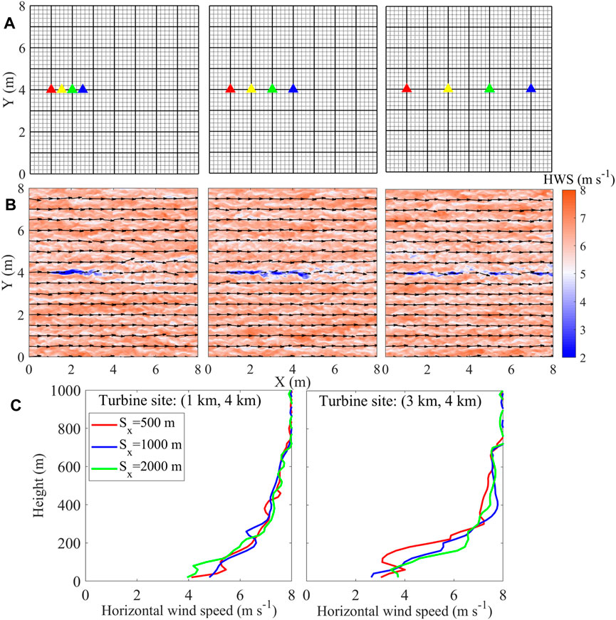
FIGURE 5. Location of four turbines in the domain: (A) (steam-wise turbine spacing of 0.5 km (case 2), 1 km (case 3), and 2 km (case 4)) and the corresponding simulated wind fields; (B) (arrow: wind vectors; shaded colors: wind speed). Vertical wind profiles (C) at (1 km, 4 km) and (3 km, 4 km), respectively.

What was striking in Figure 5 is that the linear arrangement of turbines with different spacing resulted in different wake conditions, and as expected, the power generation varied with different turbine spacing. To further study the sensitivity of the power yield to the turbine spacing, the simulated output power of cases 2–4 is compared in Figure 6. Under the wind speed of 8 m s^-1, the output power of the independent turbine is the largest, with approximately 1.5 MW (case 1), which is consistent with the power–wind speed curve shown in Figure 3. When there are four turbines in a horizontal line (case 2), the output power of turbine No. 1 in the upwind direction is the highest, close to the power of the independent turbine (mean (P₁-P₀) ∼ 0.125 MW). Turbine nos 2–4 are in the downwind direction of turbine No. 1, respectively. Considering the distance between the four turbines of 0.5 km, based on the previous discussion, the last three turbines are in the range of the “joint-wake” effect, where the wind speed is reduced to ∼3 m s^-1. According to the wind speed–power nonlinear relationship, the corresponding power generation power can be ∼0.4 MW (Figure 4C; Figure 3D). The output power of turbine nos 2–4 is significantly attenuated due to the wake effect, and the average power generation of each one decreases by ∼ 1 MW. However, when the distance between the four linearly aligned turbines is doubled to 1 km, the generated power of turbine nos 2–4 in the downwind position of turbine No. 1 slightly increased compared with that of case 2, but it is still significantly lower than the output power of the independent turbine No. 0. When the turbine spacing continued to double, that is, the distance reaches ∼2 km, the output power of all turbines increases further, especially for the turbine nos 3–4 in the most downwind position. The power generation of turbine No.1 is mostly equal to the power of that independent turbine. As each wake is independent, the wind energy in front of turbine nos 2–4 rose, with averaged power yields lowered by ∼ 0.5 MW than that of the independent turbine (P₀).

FIGURE 6

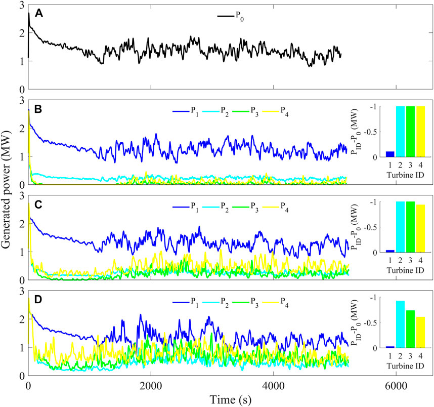
FIGURE 6. Generated power of one single turbine [case 1, (A)] and four turbines with an increasing steam-wise turbine spacing of 0.5 km [case 2, (B)], 1 km [case 3, (C)], and 2 km [case 4, (D)], respectively.

3.3 Influences of horizontal and vertical staggering wind farms

The data in Figure 7 show the results of power yields for the wind farm at different horizontal staggered angles θ (cases 5–10), as described in Table 1. The normalized average power output ratio relative to the first-row power of (P_row/P_row1) as a function of the downstream row ID for the alignment angles θ (°) equal to 26.5, 21.8, 16.7, 11.3, 5.7, and 0, respectively, is exhibited in Figure 7A. P_row1 indicates the power generation in the first row of the case (θ = 0°, y_offset = 0 m). It illustrates that with increasing θ, the generated power loss over all the rows decreases gradually. When the wind farm layout changes from a neatly arranged rectangle (θ = 0°) to an interleaving pattern with 100 m in the y-direction (θ = 5.7°), the power loss of all the rows downwind from the third row is almost unchanged. However, the power loss immediately decreases notably with the further doubling of interleaving distance in the y-direction (θ = 11.3°, y_offset = 200 m). When the staggering distance of the front and rear turbines in the y-direction is further doubled, the power loss decreases more (θ = 16.7°, y_offset = 300 m). We consider that 16.7° is very likely to be a horizontally staggered threshold at which the power generated by the wind turbine is maximized because there is little change as the degree of staggering continues to increase. Considering the lowest land cost, there exists a certain staggering degree threshold for horizontally staggered wind farms that minimizes the impact of wake effects and produces the maximum amount of power generation for a certain prevailing wind direction. Figure 7B shows the normalized average power ratio as a function of the alignment angle θ for the different turbine rows downwind. For the second turbine row, it reveals the most significant sensitivity of power loss to the alignment angles θ. The power loss decreased from ∼50% to ∼2%, with the θ increasing from 0° to 11.3°. The other rows in the downwind position have almost the same change trend and decrease the degree of power loss with an increase in θ. Surprisingly, this figure also emphasizes that for different rows in the downwind position, the power loss does not decrease anymore with the alignment angles θ ≥ 16.7°. As the data in Figure 7C show, it is apparent that the output power is sensitive to the wind farm’s layout with a horizontal staggering degree. Under the prevailing wind speed of ∼8 m s^-1, the average gross power yield could reach ∼2.7 MW with the alignment angles θ ≥ 16.7°.

FIGURE 7

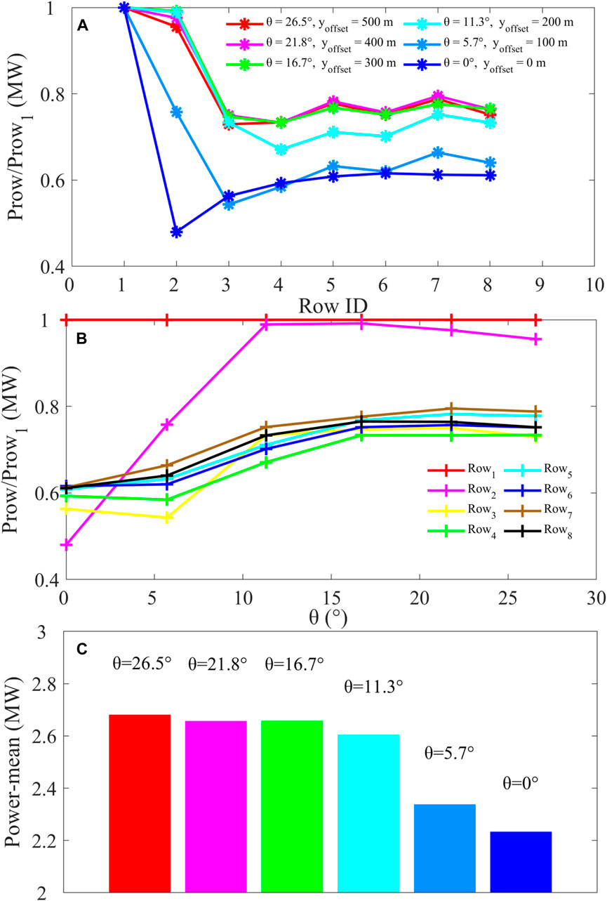
FIGURE 7. Average power output as a function of the downstream position for the different alignment angles θ (A); average power output for the different downstream turbine rows as a function of θ (B); gross average power output for the wind farms at different alignment angles θ (C).

In order to further explore the impact of vertically staggered wind farms on power generation, model tests in cases 11–17 were run, the simulation results of which are shown in Figure 8. Figure 8A shows the power generation as a function of the downstream position for different vertically staggered wind farms. The results are normalized with ratios of downstream rows relative to the power of the first row, respectively, which is denoted as P_row/P_row1. P_row1 indicates the power generation in the first row of the case (dH = 0 m). As analyzed in Section 3.1, 3.2, the power yield of the matrix wind farm with the same hub heights (H = 70 m) produces a significant drop in the second row downwind due to the wake effect. Considering the increased turbulence in the wake, further downstream, the power yield increases slightly due to the creation of a strong downward vertical kinetic energy flux that makes up for the wake’s weakening (Calaf et al., 2010). With an increase in hub heights of even-row turbines, the power generation of the even-row increases. Surprisingly, the power yields of the even rows downwind exceed that of the first row (P_row/P_row1∼ 1.1) when the hub height elevates 30 m, respectively. Meanwhile, the power yields of the odd rows change a little when the hub heights of the odd rows lower 10, 20, and 30 m, respectively.

FIGURE 8

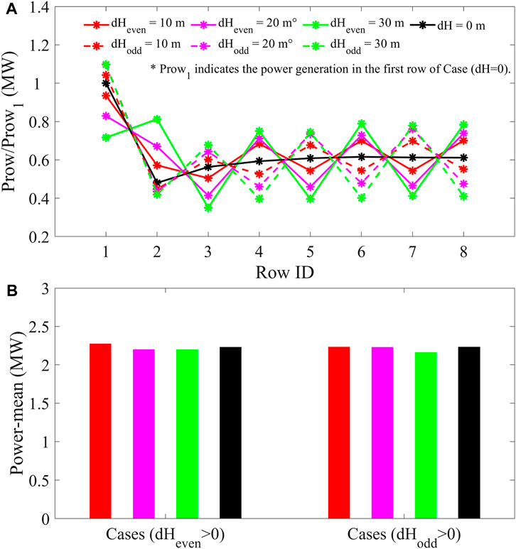
FIGURE 8. Average power output as a function of the downstream row position for the different hub height change dH (A); gross average power output for the wind farms at the different hub height change dH (B).

As discussed above, vertical staggering significantly increases the power production in the entrance region of large wind farms (in the first two rows). Surprisingly, vertical staggering does not significantly improve power production in terms of overall wind farm generation, according to the data displayed in Figure 8B. It illustrates that the average/total gross power yields of different vertically staggered wind farms are almost the same. Under the cut-in wind speed of ∼8 m s^-1, the mean gross power yield maintains the value of ∼2.25 MW and the gross power yield keeps ∼70 MW with different vertically staggered degrees (dH = 10, 20, and 30 m, respectively). Thus, wind turbines with shorter hub heights are effectively sheltered from the atmospheric flow above the wind farm that supplies the energy, which limits the benefit of vertical staggering.

After studying the generation efficiency of horizontal and vertical staggering wind farm layouts separately, the output of wind farms with both horizontal and vertical staggered layouts is further compared in Figure 9. As previously analyzed, the optimal power generation mode of horizontal staggering is case 7 with the interleaving angle of 16.7°. On this basis, vertical interleaving (dH_even = 20 m) is added, indicating that both horizontal and vertical staggering were considered at the same time, namely, case 17. As shown in Figure 9A, the results of cases 7, 10, and 17 are normalized with ratios of downstream rows relative to the power of the first row of case 10, respectively, which is denoted as P_row/P_row1. P_row1 indicates the power generation in the first row of the case (θ = 0°; dH = 0 m). The wind farm output of optimal horizontal staggering and that considering both optimal horizontal and vertical staggering significantly increase in the second row downwind, effectively reducing the influence of the wake effect, especially the latter. For wind farms considering only the optimal horizontal staggering, the wake weakening effect is significantly reduced in the remaining rows in the downwind position, and the power generation is improved compared with that of normal wind farms in case 10. However, wind farms considering both the optimal horizontal and vertical staggering at the same time only increased the power generation in the even rows, while the odd rows have no change. In order to directly compare the power yields of the three cases, Figure 9B displays the average power and total power of a wind farm using only optimal horizontal interleaving, optimal horizontal and vertical interleaving, and matrix layout, respectively. The wind farm only considering the optimal horizontal staggering mode has the highest power generation efficiency. Further vertical staggering on the optimal horizontal staggering layout will reduce the overall and average power generation efficiency. The reason could be that vertical staggering is much less beneficial in terms of overall wind farm generation than originally anticipated, as analyzed above.

FIGURE 9

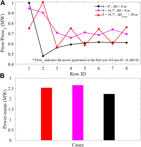
FIGURE 9. Average power output as a function of the downstream row position for the different hub height change dH and horizontal staggering angle θ (A); gross average power output for the wind farms at the different hub height change dH and alignment angles θ (B).

4 Conclusion

In this work, we used LES to identify the wake effect structures, quantify relative turbine output with various turbine spacing, and further study the effects of horizontal and vertical staggering on the power production in wind farms.

The airflow velocity through the independent turbine will be reduced by 50% in the vertical direction of the turbine diameter range, and the weakening can last for a length of ∼2 km in the horizontal direction. However, in the vertical range of the radius above the turbine, the turbulent kinetic energy increased and continued for ∼1 km in the horizontal direction. With the increase of turbine spacing in the horizontal direction, the influence of the wake effect between the turbines gradually decreases, and the relative turbine output gradually recovers, especially for the downstream turbine. With changing horizontal staggering degree simulations, the highest power output for the entire wind farm is obtained when an alignment angle θ of approximately 16.7° is used. Considering the relatively small land cost utilization, it ensures that the power output of the downwind rows is least affected by the wake effects. On the other hand, vertical staggering significantly increases the power production in the entrance region of large wind farms and does not significantly improve the power production in terms of overall wind farm generation. Through the simulation considering horizontal and vertical staggering, we find the optimal power output for the entire wind farm is obtained when the horizontal staggering degree θ of 16.7° is used and no vertical staggering is adapted. It should be noted that this work does not claim to provide or propose an optimal layout of wind farms in general. The research results have certain guiding significance for the optimal layout of wind farms in practical applications, especially in the sites with a clear dominant wind direction.

Data availability statement

The original contributions presented in the study are included in the article/Supplementary material; further inquiries can be directed to the corresponding author.

Author contributions

DZ: writing–original draft. JX: supervision and writing–review and editing. XP: writing–review and editing. YoM: writing–review and editing. XR: data curation and writing–review and editing. YJ: methodology and writing–review and editing. YMa: writing–review and editing. CG: writing–review and editing.

Funding

The author(s) declare financial support was received for the research, authorship, and/or publication of this article. This study was supported by the Basic research funds for universities and colleges (PHD2023–018), the National Natural Science Foundation of China (42307144), and the China Postdoctoral Science Foundations (2022TQ0332; 2021M700140).

Acknowledgments

The authors are thankful for the model support from the palm group in the Institute of Meteorology and Climatology, Leibniz Universität Hannover.

Conflict of interest

Author YJ was employed by Goldwind Technology Co., LTD. Author YM was employed by Shanghai Investigation, Design, and Research Institute Co., Ltd.

The remaining authors declare that the research was conducted in the absence of any commercial or financial relationships that could be construed as a potential conflict of interest.

Publisher’s note

All claims expressed in this article are solely those of the authors and do not necessarily represent those of their affiliated organizations, or those of the publisher, the editors, and the reviewers. Any product that may be evaluated in this article, or claim that may be made by its manufacturer, is not guaranteed or endorsed by the publisher.

References

Archer, C. L., Mirzaeisefat, S., and Lee, S. (2013). Quantifying the sensitivity of wind farm performance to array layout options using Large-Eddy Simulation. Geophys. Res. Lett. 40 (18), 4963–4970. doi:10.1002/grl.50911

CrossRef Full Text | Google Scholar

Barber, S., Chokani, N., and Abhari, R. S. (2011). Wind turbine performance and aerodynamics in wakes within wind farms. Brussels, Belgium: European Wind Energy Conference and Exhibition.

Google Scholar

Cal, R. B., Lebron, J., Castillo, L., Kang, H. S., and Meneveau, C. (2010). Experimental study of the horizontally averaged flow structure in a model wind-turbine array boundary layer. J. Renew. Sust. Energ. 2 (1), 013106. doi:10.1063/1.3289735

CrossRef Full Text | Google Scholar

Calaf, M., Meneveau, C., and Meyers, J. (2010). Large eddy simulation study of fully developed wind-turbine array boundary layers. Phys. Fluids. 22 (1). doi:10.1063/1.3291077

CrossRef Full Text | Google Scholar

Göçmen, T., Van der Laan, P., Réthoré, P. E., Diaz, A. P., Larsen, G. C., and Ott, S. (2016). Wind turbine wake models developed at the technical university of Denmark: a review. Renew. Sust. Energ. Rev. 60, 752–769. doi:10.1016/j.rser.2016.01.113

CrossRef Full Text | Google Scholar

Kuik, G. A. M. V., Peinke, J., Nijssen, R., Lekou, D., Skytte, K., Sørensen, J. N., et al. (2016). Long-term research challenges in wind energy-a research agenda by the european academy of wind energy. Wind Energy Sci. 1 (1), 1–39. doi:10.5194/wes-1-1-2016

CrossRef Full Text | Google Scholar

Li, Y., Xu, Z. J., Xing, Z. X., Zhou, B. W., Cui, H. Q., Liu, B. W., et al. (2020). A modified Reynolds-averaged Navier–Stokes-based wind turbine wake model considering correction modules. Energies 13 (17), 4430. doi:10.3390/en13174430

CrossRef Full Text | Google Scholar

Li, Z. B., Liu, X. H., and Yang, X. L. (2022). Review of turbine parameterization models for large-eddy simulation of wind turbine wakes. Energies 15 (18), 6533. doi:10.3390/en15186533

CrossRef Full Text | Google Scholar

Liu, W. J., and Zhang, W. Q. (2020). Research on wind power development and grid-connected technology. J. Electron. Test. 18, 2. (Chinese).

Google Scholar

Ma, Y. J., Xin, J. Y., Wang, Z. F., Tian, Y. L., Wu, L., Tang, G. Q., et al. (2021). How do aerosols above the residual layer affect the planetary boundary layer height? Sci. Total Environ. 814, 151953. doi:10.1016/j.scitotenv.2021.151953

PubMed Abstract | CrossRef Full Text | Google Scholar

Ma, Y. J., Ye, J. H., Ribeiro, I. O., Vilà-Guerau de Arellano, J., Xin, J. Y., Zhang, W., et al. (2021). Optimization and representativeness of atmospheric chemical sampling by hovering unmanned aerial vehicles over tropical forests. Earth Space Sci. 8, e2020EA001335. doi:10.1029/2020EA001335

CrossRef Full Text | Google Scholar

Ma, Y. J., Ye, J. H., Xin, J. Y., Zhang, W. Y., Vilà-Guerau de Arellano, J., Zhao, D. D., et al. (2020). The stove, dome, and umbrella effects of atmospheric aerosol on the development of the planetary boundary layer in hazy regions. Geophys. Res. Lett. 47 (13), e2020GL087373. doi:10.1029/2020GL087373

CrossRef Full Text | Google Scholar

Meyers, J., and Meneveau, C. (2013). “Large eddy simulations of large wind-turbine arrays in the atmospheric boundary layer,” in Aiaa Aerospace Sciences Meeting Including the New Horizons Forum and Aerospace Exposition, Grapevine, 07 - 10 January 2013.

Google Scholar

Qin, H. Y. (2021). The 14th Five-Year Plan was the right time to vigorously develop wind power. Wind Energy 11, 1. (Chinese). doi:10.3969/j.issn.1674-9219.2021.11.001

CrossRef Full Text | Google Scholar

Raasch, S., and Schroter, M. (2001). “A large-eddy simulation model performing on massively parallel computers,” in 15th Symposium on Boundary Layers and Turbulence, Wageningen, Netherlands, 15-19 July, 2002, 289–292.

Google Scholar

Smith, G., Schlez, W., Liddell, A., Neubert, A., and Pena, A. (2006). “Advanced wake model for very closely spaced turbines,” in European Wind Energy Conference and Exhibition (EWEC) 2006, Athens, Greece, 27 February - 2 March 2006.

Google Scholar

Stevens, R. J. A. M., Gayme, D. F., and Meneveau, C. (2014). Large eddy simulation studies of the effects of alignment and wind farm length. Sust. Energ. 6 (2), 023105. doi:10.1063/1.4869568

CrossRef Full Text | Google Scholar

Stevens, R. J. A. M., and Meneveau, C. (2020). Large eddy simulation study of extended wind farms with large inter turbine spacing. J. Phys. Conf. Ser. 1618, 062011. doi:10.1088/1742-6596/1618/6/062011

CrossRef Full Text | Google Scholar

Storey, R., Norris, S., and Cater, J. (2013). “Large eddy simulation of wind events propagating through an array of wind turbines,” in Proceedings of the World Congress on Engineering 2013 Vol III, WCE 2013, London, UK, 3-5 July 2013.

Google Scholar

Verma, S., Paul, A. R., and Jain, A. (2022). Performance investigation and energy production of a novel horizontal axis wind turbine with winglet. Int. J. Energ. Res. 46, 4947–4964. doi:10.1002/er.7488

CrossRef Full Text | Google Scholar

Verma, S., Paul, A. R., Jain, A., and Alam, F. (2021). Numerical investigation of stall characteristics for winglet blade of a horizontal axis wind turbine. E3S Web Conf. 321, 03004. doi:10.1051/e3sconf/202132103004

CrossRef Full Text | Google Scholar

Wang, F. (2021). Explore the development path of "14th Five-Year Plan" wind power under the goal of "dual carbon. Wind Energy 4. (Chinese). doi:10.3969/j.issn.1674-9219.2021.04.018

CrossRef Full Text | Google Scholar

Wang, Y. H., Ma, Y. J., Lin, Z. R., Yao, L., Cai, R. L., Zhao, X. J., et al. (2023). Sulfur dioxide transported from the residual layer drives atmospheric nucleation during haze periods in beijing. Geophys. Res. Lett. 50 (6), e2022GL100514. doi:10.1029/2022GL100514

CrossRef Full Text | Google Scholar

Witha, B., Steinfeld, G., Doerenkaemper, M., and Heinemann, D. (2014). Large-eddy simulation of multiple wakes in offshore wind farms. J. Phys. Conf. Ser. 555, 012108. doi:10.1088/1742-6596/555/1/012108

CrossRef Full Text | Google Scholar

Yang, X. L., Kang, S., and Sotiropoulos, F. (2012). Computational study and modeling of turbine spacing effects in infinite aligned wind farms. Phys. Fluids. 24 (11), 115107. doi:10.1063/1.4767727

CrossRef Full Text | Google Scholar

Yang, X. L., and Sotiropoulos, F. (2019). A review on the meandering of wind turbine wakes. Energies 12 (14), 4725. doi:10.3390/en12244725

CrossRef Full Text | Google Scholar