A robust optimization method for new distribution systems based on adaptive data-driven polyhedral sets

1 Introduction

With the high proportion of new energy access, the operation of new distribution systems is facing unprecedented challenges. Compared with traditional fossil fuel power generation, new energy is characterized by volatility and randomness, which brings an unpredictable disturbance risk to the operation of distribution systems. The traditional distribution system operation mode is based on reliable load prediction and controllable power generation methods, but the access of new energy has changed this mode (Su et al., 2018; Aenovi and Jakus, 2020).

In order to deal with the uncertainty of distributed photovoltaic (PV) output, there are mainly two uncertain optimization methods for distribution system dispatching: stochastic optimization methods (Wang et al., 2016; Torquato et al., 2018; Leng et al., 2023) and robust optimization methods (Sun et al., 2015; IsmaSmA et al., 2019). Robust optimization methods usually use the set form to describe the distribution range of uncertain parameters. Compared with stochastic methods, it does not need to obtain the probability distribution of uncertain parameters and avoids the high-dimensional problem introduced by a large number of scenarios, so it has attracted more and more attention.

However, different set forms will affect the robust optimization results of new distribution systems, so selecting an appropriate set can not only reduce the conservatism of the robust optimization results but also ensure the robustness of the results. Ding and Mather (2017), Gao et al. (2017), and Abad and Ma (2021) used the box set to describe the distribution range of uncertain parameters, and for the box set model, the worst cases were obtained only at the border. However, in reality, these conditions rarely occur, so the robust optimization methods based on the box set will have the problem of overly conservative results. Some scholars also use uncertain parameter sets to control the envelope range of uncertain parameters, thereby optimizing the conservatism of the results (Yu et al., 2016). Zhang X. et al. (2022) established a collaborative robust optimization model for reactive power optimization and reconstruction of AC/DC hybrid distribution networks, which improved the economic efficiency of distribution network operation. Xu et al. (2021) proposed a distributed robust optimization scheduling model for the interconnection and interoperability between electric vehicle clusters and power systems. Xu et al. (2021) and Zhang X. et al. (2022) used polyhedral sets to describe the envelope range of uncertain parameters, which are more conservative than interval sets. However, polyhedral sets do not consider the correlation between uncertain parameters, and their conservatism still needs improvement. Florin et al. (2015) proposed a new uncertainty set based on classification probability chance constraints to fully consider the differences in the random distribution of various uncertainty factors. This method can accurately describe the robustness of dispatching schemes so as to better deal with the effects of various uncertainties. However, for uncertain parameters with correlation, the conservatism of the above studies needs to be improved.

In recent years, in order to enhance the reliability of robust optimization results and describe the correlation between uncertain parameters, some scholars have used the historical data on uncertain variables to try finding out the relationship between random variable changes and propose a data-driven uncertainty set (Dent et al., 2010; Florin et al., 2015; Abad et al., 2018; Masoume et al., 2022). Chen et al. (2017) established a polyhedral uncertainty set based on historical wind data to model, analyze, and optimize economic dispatch. Tan et al. (2020) established a correlation polyhedral set model by bending the boundary of the polyhedral set with the method of mathematical analysis based on the polyhedral set. Taha et al. (2021) further improved the construction of a generalized correlation polyhedral set model on the basis of the study proposed in Tan et al. (2020) so that the polyhedral set can better cover the range of the occurrence of uncertain parameters. Moreira et al. (2017) constructed an elliptic set to describe the PV output, and an affinely adjustable robust optimal operation strategy for the active distribution network was proposed. Although the elliptic set can well-consider the correlation between uncertain parameters, its nonlinear structure increases the difficulty of solving the model. Although the correlation of uncertain sets is considered in Chen et al. (2017), Moreira et al. (2017), Tan et al. (2020), and Taha et al. (2021), the large envelope range of the uncertain sets they established will increase the conservatism of decision-making.

In addition to building with polyhedral and elliptic sets, another common approach is to build uncertain sets based on extreme scenarios. Zhang S. et al. (2022) and Palahalli et al. (2022) first selected the historical data on uncertain sets, then constructed convex hull sets based on extreme scenarios filtered from historical data, and introduced appropriate scaling factors to cover all historical data. Finally, a robust optimization model based on extreme scenarios is established. The method proposed by Zeng and Zhao (2013) and Chen et al. (2018) did not presuppose the shape of the uncertain set but represented the uncertain set as the convex hull of historical scenarios. The above research has improved the problem of high conservation in polyhedral sets, but the sets constructed based on extreme scenarios may face difficulties in a robust solution.

In view of the shortcomings of the above sets, a novel robust optimization method for new distribution systems based on adaptive data-driven polyhedral sets is proposed in this paper. First, the elliptic set is constructed based on the historical scenarios, then the convex hull polyhedral set is constructed by connecting the elliptic vertices, and finally all the historical scenarios are covered by scaling. In order to solve the problem of high conservation in the scaled convex hull polyhedral set, an adaptive data-driven polyhedral set based on the idea of hyperplane is constructed. Finally, the effectiveness of the proposed method is verified by an improved IEEE-33 bus system.

The rest of the paper is organized as follows: Section 2 introduces the representation methods of convex hull uncertain and hyperplane uncertain sets; Section 3 presents an economic dispatch model for the new distribution system; Section 4 uses the C&CG algorithm to construct a robust scheduling model; Section 5 uses an improved 33-node system to verify the effectiveness of the method proposed in this paper; finally, the conclusion is presented in Section 6.

2 Data-driven uncertainty set modeling

2.1 Convex hull polyhedral set

This paper first collected data on photovoltaic reception in different areas of a township city in Guangdong Province and divided the collected historical data into days. The number of days for collecting historical data was set as $N_h$, and the number of photovoltaic scenes was set as $N_w$. The daily output data were recorded as a historical scene, and the collected data were written in the form of a vector as follows: $w_k=\left(P_{1,1}^{\text{PV},k}\cdots P_{1,T}^{\text{PV},k}\cdots P_{N_w,T}^{\text{PV},k}\right),k=1,2\dots N_h$, and $T$ represents the time dimension, which is 24 h in this paper. $P_{1,t}^{\text{PV},k}$ indicates the output size of the i-th photovoltaic scene at time t in the k-th group. In practical applications, a photovoltaic data processing platform can be designed based on the historical data on the local photovoltaic output, and the required information can be obtained by inputting data. According to the scatter plot formed by the historical data on the distributed PV output, different envelope lines can be used to represent different sets, such as the box set and ellipsoid set, as shown in Figure 1. For different sets, this paper uses a budget uncertainty set $\mathit{U}$ to describe the fluctuation range of the distributed PV output.

Figure 1

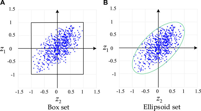
Figure 1. Uncertain set.

2.1.1 Box set

The specific expression is represented as follows:

$\mathit{U}=\left\{{\mathit{z}}^{\text{PV}}\in {\mathit{R}}^{N_{\text{PV}}\times 1}|\beta {\mathit{z}}_{\text{down}}^{\text{PV}}\le {\mathit{z}}^{\text{PV}}\le \beta {\mathit{z}}_{\text{up}}^{\text{PV}}\right\},(1)$

where $N_{\text{PV}}$ represents the number of distributed PVs; ${\mathit{z}}^{\text{PV}}$ represents the distributed PV uncertainty variable. ${\mathit{z}}_{\text{up}}^{\text{PV}}$ and ${\mathit{z}}_{\text{down}}^{\text{PV}}$ represent the upper and lower boundaries of distributed PV uncertainty variables, respectively. $\beta$ represents the adjustment coefficient, and the conservative value used to adjust the box set is $\left(0,1\right]$.

Figure 1A shows that the box set envelops all possibilities of the distributed PV output. However, because the distributed PV often has a certain temporal and spatial correlation at different times and at different locations, PV output data are mostly concentrated around the y = x and y = -x function lines. At this time, if the box set is used to describe the uncertainty of the PV output, the optimization scheme may be too conservative because the box set not only covers all possibilities of fluctuations but also covers the blank area with a low probability of fluctuations. Therefore, it is necessary to adopt a more appropriate approach to modeling uncertain sets.

2.1.2 Ellipsoid set

The specific expression is shown in Eq. (2):

$\mathit{U}=\left\{{\mathit{z}}^{\text{PV}}\in {\mathit{R}}^{N_{\text{PV}}\times 1}|{\left({\mathit{z}}^{\text{PV}}-\mathit{c}\right)}^{\mathrm{T}}{\mathrm{\Sigma }}^{-1}\left({\mathit{z}}^{\text{PV}}-\mathit{c}\right)\le 1\right\},(2)$

where $\mathit{c}$ represents the center point of the high-dimensional ellipsoid. $\mathrm{\Sigma }\in {\mathit{R}}^{N_{\text{PV}}\times N_{\text{PV}}}$ indicates a positive definite matrix that represents the offset direction of the high-dimensional ellipsoid relative to the coordinate axis.

Figure 1B shows that both the ellipsoid and box sets envelop all possibilities of the distributed PV output. At the same time, unlike the box set, the ellipsoid set reduces the blank area with a low probability of envelope fluctuation and reduces the conservative of the decision result. However, the expression of the ellipsoid set is quadratic, so it is more difficult to solve in the process of robust optimization.

On this basis, Palahalli et al. (2022) proposed a generalized convex hull set that can effectively reduce the conservatism of optimization results and avoid the introduction of quadratic forms in the modeling process. First, this method utilizes existing high-dimensional ellipsoid-solving algorithms to propose a novel data-driven uncertain set modeling method, which generates uncertain sets in the form of linear generalized convex hulls; compared with traditional box sets, generalized convex hull sets can reduce the conservatism of results by reducing the envelope of empty hull regions, while uncertain sets in linear form reduce the complexity of computational results. Therefore, this article constructs a data-driven uncertain set based on Palahalli et al. (2022), and the modeling process is shown in Figure 2.

  Step (1): First, a high-dimensional ellipsoid uncertainty set ${\mathit{U}}_{e1}$ that covers all historical data fluctuations and has the smallest volume is constructed. The constructed high-dimensional ellipsoid is shown in Figures 2A and is specifically expressed in Eq. 3:

${\mathit{U}}_{e1}=\left\{{\mathit{z}}^{\text{PV}}\in {\mathit{R}}^{N_{\text{PV}}\times 1}|{\left({\mathit{z}}^{\text{PV}}-\mathit{c}\right)}^{\mathrm{T}}{\mathrm{\Sigma }}^{-1}\left({\mathit{z}}^{\text{PV}}-\mathit{c}\right)\le 1\right\}.(3)$

  Step (2): On the basis of the original high-dimensional ellipsoid, the positive definite matrix $\mathit{\Sigma }$ is orthogonally decomposed, $\mathit{\Sigma }={\mathit{P}}^{\mathit{T}}\mathit{J}\mathit{P}={\mathit{P}}^{-1}\mathit{J}\mathit{P}$. The original ellipsoid is rotated and translated so that the center of the ellipsoid falls on the center point of the coordinate axis, as shown in the green dotted line in Figure 2B. At this time, the high-dimensional ellipsoid uncertainty set is ${\mathit{U}}_{e2}$, As shown in Eqs (4, 5):

${\mathit{U}}_{e2}=\left\{{{\mathit{z}}^{\text{PV}}}^{\prime }\in {\mathit{R}}^{N_{\text{PV}}\times 1}|{\left({{\mathit{z}}^{\text{PV}}}^{\prime }\right)}^{\mathrm{T}}{\mathit{J}}^{-1}\left({{\mathit{z}}^{\text{PV}}}^{\prime }\right)\le 1\right\},(4)$

${{\mathit{z}}^{\text{PV}}}^{\prime }=\mathit{P}\times \left({\mathit{z}}^{\text{PV}}-\mathit{c}\right),(5)$

where $\mathit{J}$ represents the diagonal matrix, denoted as $\mathit{J}=\text{diag}\left({\lambda }_1\dots {\lambda }_{N_{\text{PV}}}\right)$. $\mathit{P}$ indicates the transformation matrix, representing the offset angle of the matrix. According to the diagonal matrix $\mathit{J}$, the coordinates of the vertex ${z_{c,i}^{\text{PV}}}^{\prime }$ of the transformed high-dimensional ellipsoid are as shown in Eq. (6):

$\left\{\begin{array}{l}{z_{c,1}^{\text{PV}}}^{\prime }=\left[1/\sqrt{{\lambda }_1},0\dots 0\right],{z_{c,N_{\text{PV}}+1}^{\text{PV}}}^{\prime }=-\left[1/\sqrt{{\lambda }_1},0\dots 0\right]\\ {z_{c,2}^{\text{PV}}}^{\prime }=\left[0,1/\sqrt{{\lambda }_2}\dots 0\right],{z_{c,N_{\text{PV}}+2}^{\text{PV}}}^{\prime }=-\left[0,1/\sqrt{{\lambda }_2}\dots 0\right]\\ ⋮\\ {z_{c,N_{\text{PV}}}^{\text{PV}}}^{\prime }=\left[0,0\dots 1/\sqrt{{\lambda }_{N_{\text{PV}}}}\right],{z_{c,2N_{\text{PV}}}^{\text{PV}}}^{\prime }=-\left[0,0\dots 1/\sqrt{{\lambda }_{N_{\text{PV}}}}\right]\end{array}\right..(6)$

Figure 2

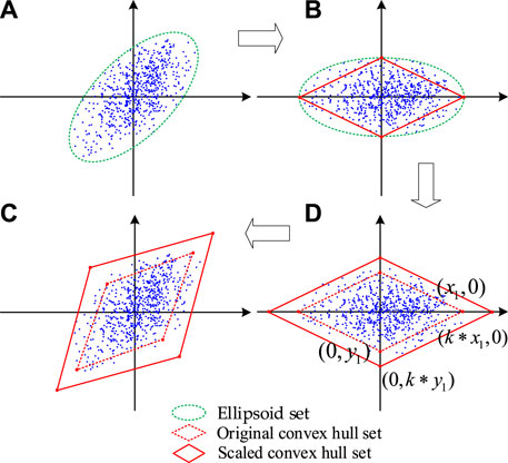
Figure 2. Modeling process of the convex hull polyhedral uncertainty set.

Furthermore, the vertices of the high-dimensional ellipsoid are connected to form a high-dimensional polyhedron, as shown by the red line in Figure 2B. At this time, the high-dimensional linear polyhedral uncertainty set ${\mathit{U}}_{p2}$ is as shown in Eq. (7):

${\mathit{U}}_{p2}=\left\{{{\mathit{z}}^{\text{PV}}}^{\prime }\in {\mathit{R}}^{N_{\text{PV}}\times 1}\left|\begin{array}{l}{{\mathit{z}}^{\text{PV}}}^{\prime }={\displaystyle \sum _{i=1}^{2N_{\text{PV}}}}{m}_i{{\mathit{z}}_{c,i}^{\text{PV}}}^{\prime }\\ {\displaystyle \sum _{i=1}^{2N_{\text{PV}}}}{m}_i=1;0\le m_i\le 1\end{array}\right.\right\},(7)$

where $m_i$ represents the weight coefficient of the i-th vertex.

  Step (3): Since the high-dimensional linear polyhedral set used in step 2 provides a small number of data points outside the envelope, it is necessary to scale the original set, as shown in the red solid line in Figure 2C. The vertices of the scaled high-dimensional linear polyhedron are as shown in Eq. (8):

$\left\{\begin{array}{l}k{z_{c,1}^{\text{PV}}}^{\prime }=\left[k/\sqrt{{\lambda }_1},0\dots 0\right],k{z_{c,N_{\text{PV}}+1}^{\text{PV}}}^{\prime }=-\left[k/\sqrt{{\lambda }_1},0\dots 0\right]\\ k{z_{c,2}^{\text{PV}}}^{\prime }=\left[0,k/\sqrt{{\lambda }_2}\dots 0\right],k{z_{c,N_{\text{PV}}+2}^{\text{PV}}}^{\prime }=-\left[0,k/\sqrt{{\lambda }_2}\dots 0\right]\\ ⋮\\ k{z_{c,N_{\text{PV}}}^{\text{PV}}}^{\prime }=\left[0,0\dots k/\sqrt{{\lambda }_{N_{\text{PV}}}}\right],k{z_{c,2N_{\text{PV}}}^{\text{PV}}}^{\prime }=-\left[0,0\dots k/\sqrt{{\lambda }_{N_{\text{PV}}}}\right]\end{array}\right.,(8)$

At this time, the scaled high-dimensional linear polyhedral uncertainty set ${\mathit{U}}_{p2}$ is represented as shown in Eq. (9):

${\mathit{U}}_{p2}=\left\{{{\mathit{z}}^{\text{PV}}}^{\prime }\in {\mathit{R}}^{N_{\text{PV}}\times 1}\left|\begin{array}{l}{{\mathit{z}}^{\text{PV}}}^{\prime }={\displaystyle \sum _{i=1}^{2N_{\text{PV}}}}{m}_{i}k{{\mathit{z}}_{c,i}^{\text{PV}}}^{\prime }\\ {\displaystyle \sum _{i=1}^{2N_{\text{PV}}}}{m}_i=1;0\le m_i\le 1\end{array}\right.\right\},(9)$

where k represents the scaling factor, which is used to adjust the conservative degree of the envelope range of the high-dimensional linear polyhedron. The calculation method of k is shown in Palahalli et al. (2022). Therefore, there is a minimum $k_{\min }$ value, which makes the scaled polyhedral set cover all possible data points, so the value range of k is $\left[0,k_{\min }\right]$. The polyhedral set formed by different k is shown in Figure 3.

  Step (4): The scaled high-dimensional linear polyhedron is rotated and translated to make it fit the range of original data points. According to (5), the high-dimensional linear polyhedral uncertainty set ${\mathit{U}}_{p1}$ after rotation and translation as shown in Eq. (10):

${\mathit{U}}_{p1}=\left\{{\mathit{z}}^{\text{PV}}\in {\mathit{R}}^{N_{\text{PV}}\times 1}\left|\begin{array}{l}{\mathit{z}}^{\text{PV}}={\displaystyle \sum _{i=1}^{2N_{\text{PV}}}}{m}_i\left(\mathit{c}+k{\mathit{P}}^{-1}{{\mathit{z}}_{c,i}^{\text{PV}}}^{\prime }\right)\\ {\displaystyle \sum _{i=1}^{2N_{\text{PV}}}}{m}_i=1;0\le m_i\le 1\end{array}\right.\right\}.(10)$

Figure 3

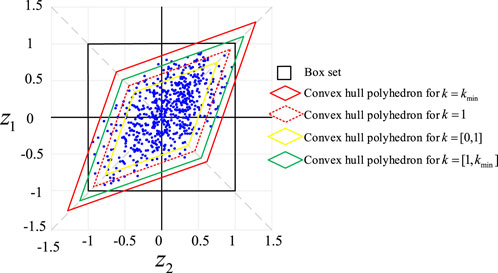
Figure 3. Range of convex hull polyhedral sets under different k-values.

2.2 Hyperplane polyhedral set

The convex hull polyhedral set introduced in Section 2.1 is used to build a high-dimensional polyhedral uncertain set connecting all vertices on the basis of establishing the ellipsoidal polyhedral set first and then make the high-dimensional polyhedral set envelop all historical data points using a scale. However, since the scale is a global scale, an excessive increase in the scaling factor may occur in order to envelope a certain data point, resulting in more blank areas being enveloped accordingly. Therefore, the uncertainty set construction method based on extreme scenarios proposed by Zeng and Zhao (2013) and Chen et al. (2018) does not determine the shape of the envelope range in advance but envelopes extreme scenarios successively to form an irregular polyhedral set, as shown in Figure 4.

Figure 4

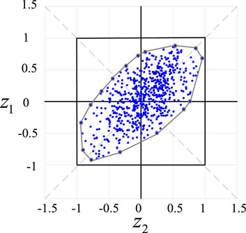
Figure 4. Uncertainty set based on extreme scenarios.

The uncertainty set expression based on extreme scenarios is represented as follows:

$\mathit{U}=\left\{{\mathit{z}}^{\text{PV}}\in {\mathit{R}}^{N_{\text{PV}}\times 1}\left|\begin{array}{l}{\mathit{z}}^{\text{PV}}={\displaystyle \sum _{i=1}^{N_{ex}}}{\sigma }_i{\mathit{z}}_i^{\text{PV}}\\ {\displaystyle \sum _{i=1}^{N_{ex}}}{\sigma }_i=1;0\le {\sigma }_i\le 1\end{array}\right.\right\},(11)$

where $N_{ex}$ represents the number of extreme scenarios; ${\mathit{z}}_i^{\text{PV}}$ represents the i-th extreme scenario; and ${\sigma }_i$ represents the weight coefficient of extreme scenarios.

Compared with the convex hull uncertainty set, the uncertainty set of extreme scenarios can greatly reduce the envelope of the blank region with small probability distribution. Therefore, this method has the best conservatism. However, it can be seen from (11) that the construction of the uncertainty set based on extreme scenarios depends on the number of extreme scenarios, i.e., the number of polyhedral vertices. If there are many extreme scenarios, it will increase the difficulty of solving robust optimization. Wu et al. (2019) proposed a set of hyperplane polyhedra. First, assuming the total dimension of the uncertainty variable is E, a closed box polyhedron is formed in the E-dimensional space that exactly covers all historical data. This closed box polyhedron is equivalent to a box uncertainty set. Starting from each vertex of the boxed uncertain set, a suitable hyperplane is found to separate the boundary of the boxed uncertain set from all historical data and maximize the removal of blank “invalid” areas in the process, as shown in Figure 5.

Figure 5

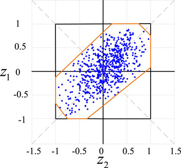
Figure 5. Hyperplane polyhedral set.

In general, for the K-dimensional space, the hyperplane is expressed as shown in Eq. (12):

${{\mathit{\alpha }}_m}^T\mathit{z}={\beta }_m,\forall m,(12)$

where ${\mathit{\alpha }}_m$ represents a K-dimensional non-zero vector; ${\beta }_m$ represents a scalar, and m represents the vertex sequence number of the K-dimensional box set. Let the vertex of the K-dimensional box set be ${\mathit{z}}_m^{\mathrm{B}}$, and the vertex generated by the hyperplane cutting the K-dimensional box set be ${\mathit{z}}_n^{\mathrm{H}}$; then, the relationship between the vertex sequence number m and n as shown in Eq. (13):

$n=\left(m-1\right)\times \mathrm{{\rm K}}+s,s=1,2\dots \mathrm{{\rm K}},\forall m=1,2\dots 2^{\mathrm{{\rm K}}}.(13)$

At this point, the vertices generated by hyperplane cutting can be obtained by solving the following model:

$\forall m,\underset{{\mathit{\alpha }}_m,{\beta }_m,{\xi }_{ms},{\mathit{z}}_n^{\mathrm{H}}}{\max }\frac{1}{\mathrm{{\rm K}}!}{\displaystyle \prod _{s=1}^{\mathrm{{\rm K}}}}{\xi }_{ms},(14)$

${{\mathit{\alpha }}_m}^T{\mathit{z}}_m^{\mathrm{B}}\ge {\beta }_m,{{\mathit{\alpha }}_m}^T\mathit{\tau }\le {\beta }_m,{{\mathit{\alpha }}_m}^T{\mathit{z}}_n^{\mathrm{H}}={\beta }_m,\forall s,\forall \mathit{\tau }\in \mathrm{{\rm T}},(15)$

$z_{mo}^{\mathrm{B}}-z_{no}^{\mathrm{H}}=0,\forall s,o=1,\dots s-1,s+1,\dots \mathrm{{\rm K}},(16)$

${\xi }_{ms}={\theta }_{ms}\left(z_{ms}^{\mathrm{B}}-z_{ns}^{\mathrm{H}}\right),\forall s,(17)$

${\xi }_{m_{1}s}+{\xi }_{m_{2}s}\le z_{m_{2}s}^{\mathrm{B}}-z_{m_{1}s}^{\mathrm{B}},\forall s,\forall h\in H\left(s\right),m_1,m_2\in h.(18)$

Equation 14 aims to solve the blank region with the maximum volume cut by the hyperplane, where ${\xi }_{ms}$ represents the geometric distance between ${\mathit{z}}_n^{\mathrm{H}}$ and the corresponding ${\mathit{z}}_m^{\mathrm{B}}$. Since (14) is a factorial form, in order to ease the calculation pressure, it is converted into the form of (19) without affecting the variables to be solved:

$\forall m,\underset{{\mathit{\alpha }}_m,{\beta }_m,{\xi }_{ms},{\mathit{z}}_n^H}{\max }{\displaystyle \sum _{s=1}^{\mathrm{{\rm K}}}}\ln {\xi }_{ms}.(19)$

Equation 15 indicates cutting the K-dimensional space into inner and outer parts, where the vertex vector ${\mathit{z}}_m^{\mathrm{B}}$ indicates that the box set is outside and the data vector $\mathit{\tau }$ is inside, and $\mathrm{{\rm T}}$ represents the dataset. Equation 16 indicates that, except for the $o=s$ dimension, the coordinate difference of other dimensions is 0; eq. 17 represents the calculation equation for the geometric distance ${\xi }_{ms}$, where the value of ${\theta }_{ms}$ is 1 or −1, obtained when ${\mathit{z}}_{ms}^{\mathrm{B}}$ is greater/less than ${\mathit{z}}_{ns}^{\mathrm{H}}$ in the s-dimension. Equation 18 represents that any two hyperplanes do not intersect in the K-dimensional box set; h and $H\left(s\right)$ represent the interval sequence number and set of the s-dimensional box uncertain set, respectively. $m_1$ and $m_2$ represent the boundary of the interval.

The above model is a nonlinear model, so the interior point method is adopted to solve it. After solving the hyperplane vertex coordinates, combined with (11), the hyperplane uncertainty set is expressed as

$\mathit{U}=\left\{{\mathit{z}}^{\mathrm{H},\text{PV}}\in {\mathit{R}}^{N_{\text{PV}}\times 1}\left|\begin{array}{l}{{\mathit{z}}^{\mathrm{H},}}^{\text{PV}}={\displaystyle \sum _{n=1}^{N_{\mathrm{H}}}}{\epsilon }_i{\mathit{z}}_n^{\mathrm{H},\text{PV}}\\ {\displaystyle \sum _{n=1}^{N_{\mathrm{H}}}}{\epsilon }_i=1;0\le {\epsilon }_i\le 1\end{array}\right.\right\},(20)$

where ${\epsilon }_i$ represents the weight coefficient of the i-th vertex.

3 Economic dispatching model for new distribution systems

3.1 Objective function

This paper considers the economic dispatch goal of minimizing the comprehensive costs of network loss cost, abandoning PV cost, and electricity purchase cost for a new distribution system, which is

$\begin{array}{l}\min C={\displaystyle \sum _{t=1}^T}{\displaystyle \sum _{ij\in L}}{c}_{\text{loss}}\left(P_{ij,t}+P_{ji,t}\right)+{\displaystyle \sum _{t=1}^T}{c}_{\text{TR}}{P}_t^{\text{TR}}+\\ {\displaystyle \sum _{t=1}^T}{\displaystyle \sum _{i\in {\mathrm{\Omega }}_N^{\text{PV}}}}{c}_{\text{PV}}\left({\stackrel{\sim }{P}}_{i,t}^{\text{PV}}-P_{i,t}^{\text{PV}}\right)\Delta t,\end{array}(21)$

where $P_{ij,t}$ and $P_{ji,t}$ represent the active power flow direction of branch ij at time t; $P_{ij,t}$ represents the power flow from bus i to bus j at time t; $P_{ji,t}$ represents the power flow from bus j to bus i; $P_t^{\text{TR}}$ represents the gateway power at time t; ${\stackrel{\sim }{P}}_{i,t}^{\text{PV}}$ represents the maximum available power of the distributed PV system connected to bus i after fluctuation at time t; $P_{i,t}^{\text{PV}}$ represents the actual injected power of the distributed PV system connected to bus i at time t; $P_{i,t}^{\text{PV}}$ represents the actual injected power of the distributed PV system connected to bus i at time t; $C$ represents the total cost of economic dispatch; $c_{\text{loss}}$ represents the cost coefficient of network loss; $c_{\text{TR}}$ represents the cost coefficient of electricity purchased for the main network at the gateway; $c_{\text{PV}}$ represents the cost coefficient of PV abandonment. ${\mathrm{\Omega }}_N^{\text{PV}}$ represents the set of bus connected to distributed PV, and $L$ represents the set of all branches of the distribution network.

3.2 Constraint condition

3.2.1 Second-order cone relaxation power flow constraints

$P_{i,t}^{\text{sum}}-P_{i,t}^{\text{cur}}={\displaystyle \sum _{j\in N\left(i\right)}}{P}_{ij,t},(22)$

$Q_{i,t}^{\text{sum}}-Q_{i,t}^{\mathrm{D}}={\displaystyle \sum _{j\in N\left(i\right)}}{Q}_{ij,t},(23)$

$P_{i,t}^{\text{sum}}=P_t^{\text{TR}}+P_{i,t}^{\text{PV}}-P_{i,t}^{\text{ch}}+P_{i,t}^{\text{dis}},(24)$

$Q_{i,t}^{\text{sum}}=Q_t^{\text{TR}}+Q_{i,t}^{\text{CB}},(25)$

$P_{ij,t}=\sqrt{2}{g}_l{u}_{i,t}-g_l{R}_{l,t}-b_l{T}_{l,t},(26)$

$P_{ji,t}=\sqrt{2}{g}_l{u}_{j,t}-g_l{R}_{l,t}+b_l{T}_{l,t},(27)$

$Q_{ij,t}=-\sqrt{2}{b}_l{u}_{i,t}+b_l{R}_{l,t}-g_l{T}_{l,t},(28)$

$Q_{ji,t}=-\sqrt{2}{b}_l{u}_{j,t}+b_l{R}_{l,t}+g_l{T}_{l,t},(29)$

$I_{l,t}^2=\sqrt{2}\left(g_l^2+b_l^2\right)\left(u_{i,t}+u_{j,t}-\sqrt{2}{R}_{l,t}\right),(30)$

$‖\begin{array}{l}\sqrt{2}{R}_{l,t}\\ \sqrt{2}{T}_{l,t}\\ u_{i,t}-u_{j,t}\end{array}‖\le u_{i,t}+u_{j,t},(31)$

$\frac{{\left(V_i^{\min }\right)}^2}{\sqrt{2}}\le u_{i,t}\le \frac{{\left(V_i^{\max }\right)}^2}{\sqrt{2}},(32)$

$I_{l,t}\le I_l^{\max }.(33)$

Equations 17–25 represent the power balance constraints of the branch, where $P_{i,t}^{\text{sum}}$ represents the total active power injected by bus i at time t. It includes the active power injected by the gateway at time t, the output power of distributed PV connected to bus i at time t, and the charging power $P_{i,t}^{\text{ch}}$ and discharging power $P_{i,t}^{\text{dis}}$ of the energy storage battery connected to bus i at time t. $P_{i,t}^{\text{cur}}$ represents the load of bus i after implementing the demand-side response at time t; $Q_{i,t}^{\text{sum}}$ represents the total reactive power injected by bus i at time t, including the reactive power $Q_t^{\text{TR}}$ injected by the gateway at time t and the reactive compensation power $Q_{i,t}^{\text{CB}}$ of the reactive power compensator connected to bus i at time t. $Q_{i,t}^{\mathrm{D}}$ represents the reactive load of bus i at time t, $Q_{ij,t}$ represents the reactive power flow of branch ij at time t, and $N\left(i\right)$ represents the set of all bus connected to bus i. Equations 26–30 represents the active/reactive power of the branch and the amplitude of the branch current, where $g_l$ and $b_l$ represent the conductance and admittance of the branch l, respectively, and $I_{l,t}$ represents the current amplitude of the branch l at time t. Meanwhile, introducing $u_{i,t}=V_{i,t}^2/\sqrt{2}$, $u_{j,t}=V_{j,t}^2/\sqrt{2}$, $R_{l,t}=V_{i,t}{V}_{j,t}\cos {\theta }_{l,t}$, and $T_{l,t}=V_{i,t}{V}_{j,t}\sin {\theta }_{l,t}$, where $V_{i,t}$ and $V_{j,t}$ represent the voltage amplitude of the head bus i and the end bus j of branch l at time t, respectively, ${\theta }_{l,t}$ represents the voltage phase angle of both ends of branch l at time t. Equation 31 is a second-order cone relaxation constraint. Equations 32–33 represent the amplitude constraints of voltage and current, where $V_i^{\min }$ and $V_i^{\max }$ represent the maximum and minimum voltage amplitude of bus i, respectively, and $I_l^{\max }$ represents the maximum current amplitude of branch l.

3.2.2 Distributed PV constraints

${\stackrel{\sim }{P}}_{i,t}^{\text{PV}}=P_{i,t}^{\text{PV},\mathrm{f}}+\Delta P^{\text{PV},\max }{z}_{i,t}^{\text{PV}},(34)$

$0\le P_{i,t}^{\text{PV}}\le {\stackrel{\sim }{P}}_{i,t}^{\text{PV}},\forall i\in {\mathrm{\Omega }}_N^{\text{PV}},(35)$

${\left(P_{i,t}^{\text{PV}}\right)}^2+{\left(Q_{i,t}^{\text{PV}}\right)}^2\le {\left(S_{i,t}^{\text{PV}}\right)}^2,\forall i\in {\mathrm{\Omega }}_N^{\text{PV}}.(36)$

Equations 34–36 represent the operation constraints of distributed PV, where $P_{i,t}^{\text{PV},\mathrm{f}}$ represents the maximum available power of the distributed PV connected to bus i before fluctuation at time t; $\Delta P^{\text{PV},\max }$ represents the maximum fluctuation of distributed PV; $Q_{i,t}^{\text{PV}}$ and $S_{i,t}^{\text{PV}}$ represent the reactive power and capacity of distributed PV connected to bus i at time t.

3.2.3 Battery energy storage constraints

$S_{i,t}^{\text{SOC}}=S_{i,t-1}^{\text{SOC}}+{\eta }_{i,\text{ch}}\frac{P_{i,t}^{\text{ch}}\Delta t}{E_{i,\max }}-\frac{P_{i,t}^{\text{dis}}\Delta t}{{\eta }_{i,\text{dis}}{E}_{i,\max }},\forall t\in H,(37)$

$\left\{\begin{array}{l}0\le P_{i,t}^{\text{ch}}\le P_{i,\max }^{\text{ch}}{D}_{i,t}^{\text{ch}}\\ 0\le P_{i,t}^{\text{dis}}\le P_{i,\max }^{\text{dis}}{D}_{i,t}^{\text{dis}}\\ D_{i,t}^{\text{ch}}+D_{i,t}^{\text{dis}}\le 1\end{array}\right.,(38)$

$S_{i,\min }^{\text{SOC}}\le S_{i,t}^{\text{SOC}}\le S_{i,\max }^{\text{SOC}}.(39)$

Equations 37–39 represent the operation constraints of battery energy storage, where $S_{i,t}^{\text{SOC}}$ represents the state of charging of battery energy storage connected to bus i at time t; $D_{i,t}^{\text{ch}}$ and $D_{i,t}^{\text{dis}}$ represent 0–1 variables, representing the charging and discharging states of the battery storage connected to bus i at time t, respectively, where 1 represents charging and 0 represents discharging; ${\eta }_{i,\text{ch}}$ and ${\eta }_{i,\text{dis}}$ represent the charging and discharging efficiencies of the battery energy storage connected to bus i, respectively. $E_{i,\max }$ represents the maximum amount of energy stored by the battery of bus i. $S_{i,\min }^{\text{SOC}}$ and $S_{i,\max }^{\text{SOC}}$ represent the minimum and maximum values of the state of battery energy storage connected to bus i, respectively. $\Delta t$ represents the battery energy storage dispatching interval, and $H$ represents the charging and discharging time set of the battery energy storage.

3.2.4 Capacitor bank operation constraints

$\left\{\begin{array}{l}0\le x_{i,t}^{\mathrm{C}}\le x_{i,\max }^{\mathrm{C}},i\in {\mathrm{\Omega }}_N^{\text{CB}}\\ Q_{i,t}^{\text{CB}}=x_{i,t}^{\mathrm{C}}{C}_{i,\text{step}},i\in {\mathrm{\Omega }}_N^{\text{CB}}\end{array}\right.,(40)$

${\displaystyle \sum _{t=1}^T}\left|x_{i,t}^{\mathrm{C}}-x_{i,t-1}^{\mathrm{C}}\right|\le {\Delta }_{\max }^{\text{CB}}.(41)$

In eqs 40–41, $x_{i,t}^{\mathrm{C}}$ represents the number of groups of capacitor connected to bus i at time t; $C_{i,\text{step}}$ represents the capacity of each group of capacitor connected to bus i; ${\mathrm{\Omega }}_N^{\text{CB}}$ represents the set of all installed capacitor bank bus; and ${\Delta }_{\max }^{\text{CB}}$ represents the maximum value of the change in the number of capacitor input groups in adjacent time periods.

3.2.5 On-load tap changer constraints

The schematic diagram of the on-load tap changer branch is shown in Figure 6:

$u_{m,t}=t_{ij}^2{u}_{j,t},(42)$

$t_{ij}=t_{ij}^{\min }+T_{ij}\Delta t_{ij},(43)$

$0\le T_{ij}\le K_{ij},(44)$

$\Delta t_{ij}=\left(t_{ij}^{\max }-t_{ij}^{\min }\right)/K_{ij}.(45)$

In eqs 42–45, $t_{ij}$ represents the transformer ratio on branch ij; $T_{ij}$ denotes an integer variable that represents the optimal gear position of the transformer. $\Delta t_{ij}$ represents the change value of each gear of the transformer tap. $K_{ij}$ represents the number of gears of the transformer tap. $t_{ij}^{\max }$ and $t_{ij}^{\min }$ represent the upper and lower limits of the transformer ratio, respectively, where $u_{m,t}={\left(V_{m,t}\right)}^2/\sqrt{2}$, $u_{j,t}={\left(V_{j,t}\right)}^2/\sqrt{2}$, and $u_{i,t}={\left(V_{i,t}\right)}^2/\sqrt{2}$.

Figure 6

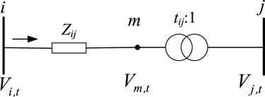
Figure 6. Schematic diagram of branches with OLTC.

3.2.6 AC/DC converter constraints

Figure 7 shows a schematic diagram of the AC/DC converter.

Figure 7

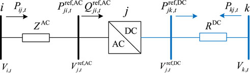
Figure 7. Schematic diagram of the AC/DC converter station.

The active power of the AC side of the converter is set at time t as $P_{ji,t}^{\text{ref},\text{AC}}$, the reactive power as $Q_{ji,t}^{\text{ref},\text{AC}}$, and the reference point voltage as $V_{j,t}^{\text{ref},\text{AC}}$. The active power of the DC side at time t is $P_{jk,t}^{\text{ref},\text{DC}}$, and the reference point voltage is $V_{j,t}^{\text{ref},\text{DC}}$. Meanwhile, $u_{j,t}^{\text{ref},\text{AC}}={\left(V_{j,t}^{\text{ref},\text{AC}}\right)}^2/\sqrt{2}$ and $u_{j,t}^{\text{ref},\text{DC}}={\left(V_{j,t}^{\text{ref},\text{DC}}\right)}^2/\sqrt{2}$ are introduced. Similar to the AC power flow in polar coordinates, the branch power flow equations with an AC/DC converter can be written as follows:

$P_{ij,t}=\sqrt{2}{g}_l{u}_{i,t}-g_l{R}_{l,t}-b_l{T}_{l,t},\forall l\in {\mathrm{\Omega }}_L^{\text{ref}},(46)$

$P_{ji,t}^{\text{ref},\text{AC}}=-\left(\sqrt{2}{g}_l{u}_{j,t}^{\text{ref},\text{AC}}-g_l{R}_{l,t}+b_l{T}_{l,t}\right),\forall l\in {\mathrm{\Omega }}_L^{\text{ref}},(47)$

$Q_{ij,t}=-\sqrt{2}{b}_l{u}_{i,t}+b_l{R}_{l,t}-g_l{T}_{l,t},\forall l\in {\mathrm{\Omega }}_L^{\text{ref}},(48)$

$Q_{ji,t}^{\text{ref},\text{AC}}=-\left(-\sqrt{2}{b}_l{u}_{j,t}^{\text{ref},\text{AC}}+b_l{R}_{l,t}+g_l{T}_{l,t}\right),\forall l\in {\mathrm{\Omega }}_L^{\text{ref}},(49)$

$P_{jk,t}^{\text{ref},\text{DC}}=\sqrt{2}{g}_l{u}_{j,t}^{\text{ref},\text{DC}}-g_l{R}_{l,t},\forall l\in {\mathrm{\Omega }}_L^{\text{ref}},(50)$

$P_{kj,t}=\sqrt{2}{g}_l{u}_{k,t}-g_l{R}_{l,t},\forall l\in {\mathrm{\Omega }}_L^{\text{ref}}.(51)$

In eqs 46–51, ${\mathrm{\Omega }}_L^{\text{ref}}$ represents the set of converter branches.

The voltage amplitude relation between AC and DC sides of the converter station as shown in Eq. (52):

$V_{j,t}^{\text{ref},\text{AC}}=K_{\mathrm{c}}{M}_i{V}_{j,t}^{\text{ref},\text{DC}},(52)$

where $K_{\mathrm{c}}$ represents the utilization rate of DC voltage; $M_i$ represents the modulation degree. The relationship between the active power of the AC and DC sides of the converter station as shown in Eq. (53):

$P_{ji,t}^{\text{ref},\text{AC}}=\frac{P_{ji,t}^{\text{ref},\text{DC}}}{{\eta }^{\text{Conv}}},(53)$

where ${\eta }^{\text{Conv}}$ represents the conversion efficiency.

3.2.7 Demand-side response constraints

$-{\xi }_{i,t}=\frac{\Delta P_{i,t}^{\mathrm{D}}}{\Delta {\rho }_t}=\frac{P_{i,t}^{\text{cur}}-P_{i,t}^{\mathrm{D}}}{{\rho }_t^{\text{cur}}-{\rho }_t},(54)$

${\displaystyle \sum _{i=1}^{N_i}}{\displaystyle \sum _{t=1}^T}{P}_{i,t}^{\text{cur}}={\displaystyle \sum _{i=1}^{N_i}}{\displaystyle \sum _{t=1}^T}{P}_{i,t}^{\mathrm{D}},(55)$

${\rho }_t^{\text{cur},\max }\le {\rho }_t^{\text{cur}}\le {\rho }_t^{\text{cur},\min },(56)$

${\rho }_t^{\text{cur}}=\left\{\begin{array}{l}{\rho }^{\text{peak}}t\in T^{\text{peak}}\\ {\rho }^{\text{valley}}t\in T^{\text{valley}}\end{array}\right..(57)$

In eqs 54–57, ${\xi }_{i,t}$ represents the elastic coefficient of electricity price of bus i at time t; $\Delta P_{i,t}^{\mathrm{D}}$ represents the change in the load of bus i before and after implementing the demand-side response at time t; $P_{i,t}^{\mathrm{D}}$ represents the load of bus i before implementing the demand-side response at time t. $\Delta {\rho }_t$ represents the change in electricity price before and after implementing the demand-side response at time t; ${\rho }_t$ and ${\rho }_t^{\text{cur}}$ represent the electricity price before and after implementing the demand-side response at time t, respectively. ${\rho }_t^{\text{cur},\max }$ and ${\rho }_t^{\text{cur},\min }$ represent the upper and lower limits of electricity price before and after implementing the demand-side response at time t, respectively. ${\rho }^{\text{peak}}$ and ${\rho }^{\text{valley}}$ represent the peak and valley electricity price before and after implementing the demand-side response at time t, respectively. $T^{\text{peak}}$ and $T^{\text{valley}}$ represent the peak and valley period before and after implementing demand-side response at time t, respectively (He et al., 2021; Qiu et al., 2021).

4 Robust dispatching method for new distribution systems

4.1 Robust dispatching model for new distribution systems

Let the constraint variable of power flow be the vector $\mathit{P}=\left\{P_{ij,t},P_{ji,t},Q_{ij,t},Q_{ji,t},P_t^{\text{TR}},Q_t^{\text{TR}},u_{i,t},R_{l,t},T_{l,t},I_{l,t}\right\}$; the constraint variable of PV is the vector ${\mathit{P}}^{\text{PV}}=\left\{P_{i,t}^{\text{PV}},Q_{i,t}^{\text{PV}}\right\}$; the variable of battery energy storage operation is the vector ${\mathit{P}}^{\text{ESS}}=\left\{S_{i,t}^{\text{SOC}},P_{i,t}^{\text{ch}},P_{i,t}^{\text{dis}}\right\}$; the operating variable of the capacitor bank is the vector ${\mathit{Q}}^{\text{CB}}=\left\{Q_{i,t}^{\text{CB}}\right\}$; the constraint variable of the on-load tap changer is the vector ${\mathit{U}}^{\text{OLTC}}=\left\{u_{m,t},t_{ij}\right\}$; the constraint variable of the AC/DC converter is the vector $\mathit{I}=\left\{P_{ji,t}^{\text{ref},\text{AC}},P_{jk,t}^{\text{ref},\text{DC}},Q_{ji,t}^{\text{ref},\text{AC}},u_{j,t}^{\text{ref},\text{AC}},u_{j,t}^{\text{ref},\text{DC}}\right\}$; and the constraint variable of a demand-side response is the vector ${\mathit{P}}^{\mathrm{D}}=\left\{P_{i,t}^{\text{cur}},{\rho }_t^{\text{cur}}\right\}$.

Based on the data-driven polyhedral set of the distributed PV output, a two-stage robust economic dispatching model for new distribution systems is established in this paper. The matrix form is as follows:

$\begin{array}{l}\underset{x}{\min }\left(\underset{u\in \mathit{U}}{\max }\underset{\mathit{y}\in \mathrm{\Omega }\left(\mathit{x},\mathit{u}\right)}{\min }{\mathit{c}}^{\mathrm{T}}\mathit{y}\right)\\ s.t.\mathit{A}\mathit{x}\le \mathit{d}\left(\mathrm{a}\right)\\ \mathit{G}\mathit{y}\le \mathit{h}-\mathit{E}\mathit{x}-\mathit{M}\mathit{u}\left(\mathrm{b}\right)\\ {‖\mathit{R}\mathit{y}‖}_2\le {\mathit{r}}^{\mathrm{T}}\mathit{y}\left(\mathrm{c}\right),\end{array}(58)$

where $\mathit{x},\mathit{y}$ represent the decision variables of the model, and $\mathit{u}$ represents an uncertainty variable. The decision variable in the first stage is $\mathit{x}=\left\{D_{i,t}^{\text{ch}},D_{i,t}^{\text{dis}},x_{i,t}^{\mathrm{C}},T_{ij}\right\}$; the decision variable in the second stage is $\mathit{y}=\left\{\mathit{P},{\mathit{P}}^{\text{PV}},{\mathit{P}}^{\text{ESS}},{\mathit{Q}}^{\text{CB}},{\mathit{U}}^{\text{OLTC}},\mathit{I},{\mathit{P}}^{\mathrm{D}}\right\}$; the uncertainty variable in the second stage is $\mathit{u}=\left\{{\stackrel{\sim }{P}}_{i,t}^{\text{PV}}\right\}$. The constant matrix $\mathit{A}$ represents the coefficient matrix associated with the decision variable $\mathit{x}$, and the column vector $\mathit{d}$ represents the coefficient vector associated with the decision variable $\mathit{x}$. The constant matrices $\mathit{G}$, $\mathit{E}$, and $\mathit{R}$ represent the coefficient matrix related to the decision variable $\mathit{y}$. The column vectors $\mathit{h}$ and $\mathit{r}$ are constant vectors representing the coefficient vector related to the decision variable $\mathit{y}$. The constant matrix $\mathit{M}$ represents the coefficient matrix associated with the uncertain variable $\mathit{u}$. $\mathrm{\Omega }\left(\mathit{y},\mathit{u}\right)$ represents the feasible region of the continuous variable $\mathit{y}$ when $\left(\mathit{x},\mathit{u}\right)$ is given. ${\mathit{c}}^{\mathrm{T}}\mathit{y}$ represents the objective function of the second stage, corresponding to (18); (54-a) corresponds to the constraints related to the variable $\mathit{x}$ in the first stage; (54-b) corresponds to the constraints related to the variable $\mathit{y}$ in the second stage; (54-c) corresponds to second-order cone constraints related to the variable $\mathit{y}$ in the second stage.

For a two-stage robust optimization model such as (58), it cannot be directly solved due to the presence of both continuous and integer variables, and the uncertain parameter $\mathit{u}$ in the second stage of the model. Therefore, this paper adopts the C&CG method (Qiu et al., 2020; Wang et al., 2021) to transform it into a master-sub problem for solving. Among them, the master problem is to solve the new distribution system robust scheduling model with the minimum comprehensive cost in the worst case scenario. After solving the integer solution of the master problem first (including the charging and discharging states of the energy storage battery, the number of capacitor bank groups, and the gear change of the on-load tap changer), the sub-problem minimizes the comprehensive cost of the system in the worst case scenario by optimizing the remaining continuous variables.

4.2 C&CG iterative solving method

4.2.1 Master–sub problem model

The master–sub problem model corresponding to (58) is as follows:

$\text{MP}1:\left\{\begin{array}{l}\underset{x,y,u}{\min }\left(\eta \right)\\ s.t.\mathit{A}\mathit{x}\le \mathit{d}\\ \mathit{G}{\mathit{y}}^l\le \mathit{h}-\mathit{E}\mathit{x}-\mathit{M}{\mathit{u}}^l\forall l\le k\\ {‖\mathit{R}{\mathit{y}}^l‖}_2\le {\mathit{r}}^{\mathrm{T}}{\mathit{y}}^l\forall l\le k\\ \eta \ge {\mathit{c}}^{\mathrm{T}}{\mathit{y}}^l\forall l\le k\end{array}\right.,(59)$

$\text{SP}1:\left\{\begin{array}{l}\underset{u\in \mathit{U}}{\max }\underset{y\in \mathrm{\Omega }\left(x,u\right)}{\min }{\mathit{c}}^{\mathrm{T}}\mathit{y}\\ s.t.\mathit{G}\mathit{y}\le \mathit{h}-\mathit{E}{\mathit{x}}^{*}-\mathit{M}\mathit{u}:\mathit{\pi }\\ {‖\mathit{R}\mathit{y}‖}_2\le {\mathit{r}}^{\mathrm{T}}\mathit{y}:{\mathit{\tau }}^a,{\mathit{\tau }}^b\end{array}\right..(60)$

First, the master problem MP1 is solved corresponding to (59). In this case, MP1 belongs to the mixed-integer second-order cone programming problem. The first stage variable solution ${\mathit{x}}^{*}$ corresponding to MP1 and the auxiliary variable $\eta$ introduced in the k+1 iteration are C&CG cuts. Then, the variable solution ${\mathit{x}}^{*}$ obtained in the first stage is substituted into the second-stage subproblem SP1 to find the worst scenario ${\mathit{u}}^l$, where l represents the number of historical iterations and k represents the number of current iterations. Finally, the worst scenario ${\mathit{u}}^l$ obtained in the second stage is brought into the master problem MP1 in the first stage for iteration. The last three constraints of (59) are the optimal cut plane and the feasible cut plane set generated by the previous k iterations, respectively. $\mathit{\pi }$, ${\mathit{\tau }}^a$, and ${\mathit{\tau }}^b$ are the dual variables of the subproblem constraints.

4.2.2 Sub-problem solving method

Equation 60 is a max–min optimization problem. Therefore, the duality theorem is used in this paper to convert the inner min problem of (60) into its dual form and combine it into a maximization problem. The specific form is shown in (61):

$\left\{\begin{array}{l}\underset{u,\pi }{\max }-{\left(\mathit{h}-\mathit{M}\mathit{u}-\mathit{E}\mathit{x}\right)}^{\mathrm{T}}\mathit{\pi }\\ s.t.\mathit{c}+{\mathit{N}}^{\mathrm{T}}\mathit{\pi }+{\mathit{R}}^{\mathrm{T}}{\mathit{\tau }}^a+\mathit{r}{\mathit{\tau }}^b=0\\ {‖{\mathit{\tau }}^a‖}_2\le {\mathit{\tau }}^b\\ \mathit{\pi },{\mathit{\tau }}^a,{\mathit{\tau }}^b\ge 0\end{array}\right..(61)$

In eq. 61, there exists a bilinear term ${\left(\mathit{M}\mathit{u}\right)}^{\mathrm{T}}\mathit{\pi }$, which is solved by the external approximation method of the bilinear term (Kersting, 2010). The master problem MP2 and the sub-problem SP2 are obtained, as shown in (62) and (63):

$\text{SP}2:\left\{\begin{array}{l}\underset{u,\pi }{\max }-{\left(\mathit{h}-\mathit{M}\mathit{u}-\mathit{E}\mathit{x}\right)}^{\mathrm{T}}\mathit{\pi }\\ s.t.\mathit{c}+{\mathit{N}}^{\mathrm{T}}\mathit{\pi }+{\mathit{R}}^{\mathrm{T}}{\mathit{\tau }}^a+\mathit{r}{\mathit{\tau }}^b=0\\ {‖{\mathit{\tau }}^a‖}_2\le {\mathit{\tau }}^b\\ \mathit{\pi },{\mathit{\tau }}^a,{\mathit{\tau }}^b\ge 0\end{array}\right.,(62)$

$\text{MP}2:\left\{\begin{array}{l}\underset{u,\pi }{\max }-{\left(\mathit{h}-\mathit{E}\mathit{x}\right)}^{\mathrm{T}}\mathit{\pi }+\mathit{\beta }\\ s.t.\mathit{c}+{\mathit{N}}^{\mathrm{T}}\mathit{\pi }+{\mathit{R}}^{\mathrm{T}}{\mathit{\tau }}^a+\mathit{r}{\mathit{\tau }}^b=0\\ {‖{\mathit{\tau }}^a‖}_2\le {\mathit{\tau }}^b\\ \mathit{\pi },{\mathit{\tau }}^a,{\mathit{\tau }}^b\ge 0\\ \mathit{\beta }\le G^m\left(\mathit{u},\mathit{\pi }\right),\forall m\le n\end{array}\right..(63)$

In eqs 62 and 63, MP2 and SP2 are used to solve the upper and lower bounds of (61), respectively, where m represents the number of historical iterations and n represents the number of current iterations. The auxiliary variable $\mathit{\beta }$ is introduced to replace the bilinear term in the original equation. The bilinear term exists in $G^m\left(\mathit{u},\mathit{\pi }\right)={\left(\mathit{M}\mathit{u}\right)}^{\mathrm{T}}\mathit{\pi }$ in (63). Therefore, the outer layer approximation method is needed for linearization, and the linearization equation is shown in (64):

$G^n\left(\mathit{u},\mathit{\pi }\right)={\left({\mathit{u}}^n\right)}^{\mathrm{T}}{\mathit{\pi }}_{sp}^n+{\left(\mathit{u}-{\mathit{u}}^n\right)}^{\mathrm{T}}{\mathit{\pi }}_{sp}^n+{\left(\mathit{\pi }-{\mathit{\pi }}_{sp}^n\right)}^{\mathrm{T}}{\mathit{u}}^n.(64)$

4.3 Solving steps and processes

The specific steps for solving the C&CG algorithm are as follows:

1) Let the initial values of the upper and lower bounds of the master-sub problem be $U1=+\infty$ and $L1=-\infty$, the initial number of iterations k = 1, and the convergence value be $\epsilon 1^{\max }$.

2) Solving the master problem in the worst case scenario, where the constraints of the master problem do not include C&CG cuts, then the integer solution ${\mathit{x}}^{*}$ is obtained.

3) Based on the integer solution ${\mathit{x}}^{*}$ obtained by solving the master problem, the sub-problem is solved to obtain the worst scenario ${\left({\mathit{u}}^{l+1}\right)}^{*}$ and the objective function value of the sub-problem. The upper limit $U1=\min \left(U1,{\mathit{c}}^{\mathrm{T}}\mathit{y}\right)$ is updated.

4) Then, whether $U1-L1$ is less than the convergence value $\epsilon 1^{\max }$ is checked. If so, the operation ends. If this is not true, $k=k+1$ is set, and a new set of scenario variables ${\mathit{u}}^k$ and C&CG cuts are added to the master problem. Solving the master problem to obtain ${\eta }^{*}$ and update the lower bound $L1=\max \left(L1,{\eta }^{*}\right)$, then step 3 is repeated.

The specific solving steps are shown in Figure 8.

Figure 8

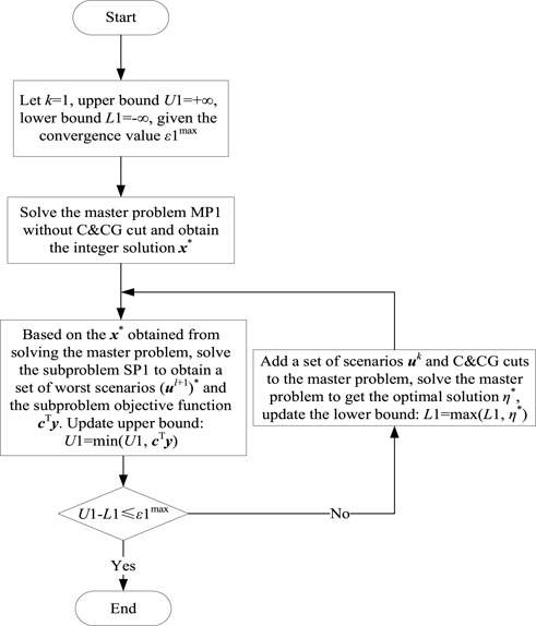
Figure 8. Solution flowchart of C&CG.

5 Example analysis

5.1 Example system settings

In order to verify the feasibility of the new distribution system optimization method based on the adaptive data-driven polyhedral set, in this section, the improved IEEE-33 bus system is used for example analysis. The wiring diagram of the improved IEEE-33 bus system is shown in Figure 9. Table 1 shows the parameter settings of PV, BESS, CB, and OLTC of the access system. The reference voltage of the system is 12.66 kV, and the reference capacity is 10 MVA. The active power range of the gateway is 0–2000 kW, the reactive power range is 0–2000 kVAr, the upper limit of the branch current amplitude is 0.5 p.u., and the bus voltage amplitude is 0.95–1.05 p.u. For the convenience of the analysis, this paper assumes that the available power of the two distributed PV systems is the same before the fluctuation and the demand-side response only for the load of the residential and commercial areas. According to the calculation method given by Palahalli et al. (2022), the value of $k_{\min }$ here is 1.41.

Figure 9

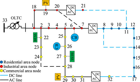
Figure 9. Modified IEEE-33 bus test system.

Table 1

Table 1. System configuration parameters.

5.2 Analysis of 33-bus system examples

5.2.1 The impact of the scaling factor k on optimization results

The influence of the scaling factor k on the robust dispatching results of the new distribution system is shown in Table 2. The size of the scaling factor k determines the coverage degree of the constructed convex hull polyhedral set to the historical data. It is not difficult to observe from Table 2 that the network loss cost is almost unchanged, the electricity purchase cost and the penalty cost of abandoning PV are slightly increasing, and the total system cost is constantly increasing. This is because, when the scaling factor k becomes larger, the convex hull uncertainty set will continue to expand the envelope range of historical output data. In other words, the fluctuation range of the distributed PV output will continue to grow, making it more prone to the worst scenario. When the distributed PV output with large fluctuations is continuously injected into the distribution network, the system needs to filter out most of the distributed PV power injection in order to meet the balance of supply and demand and reduce the disturbance caused by uncertain energy injection, so the penalty cost of abandoning PV is constantly increasing. At the same time, due to the significant reduction in the injection of distributed energy, in order to meet the power supply of the system, it is necessary to increase the injection power of the gateway, so the cost of electricity purchase gradually increases. The network loss cost depends on the network parameters of the system, so the network loss cost is almost constant. The total cost of the system is mainly the cost of abandoning PV and the cost of purchasing electricity, so the total cost of the system continues to increase.

Table 2

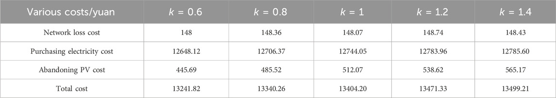
Table 2. Impact of the scaling factor k on various costs.

5.2.2 The impact of the robust adjustment coefficient $\beta$ on optimization results

Figure 10 shows the impact of the robust adjustment coefficient on the dispatching results of the new distribution system. As can be seen from the figure, with the robust adjustment coefficient increasing from 0.2 to 1, the network loss cost of the system remains almost unchanged at approximately 148 yuan, but the total cost of the system continues to increase. When the box set is adopted, the variation amplitude of the total system cost is basically stable with the increase in the robust adjustment coefficient $\beta$. When convex hull polyhedral sets with different scaling factors are used, the variation range of the total system cost decreases gradually. Specifically, when the scaling factor k changes from 0.6 to 1.4, the change amplitude of the total system cost tends to flatten out at 0.4, 0.6, and 0.8. The reason for this phenomenon is related to the change in electricity purchase and PV abandonment costs, which constitute the total cost of the system.

Figure 10

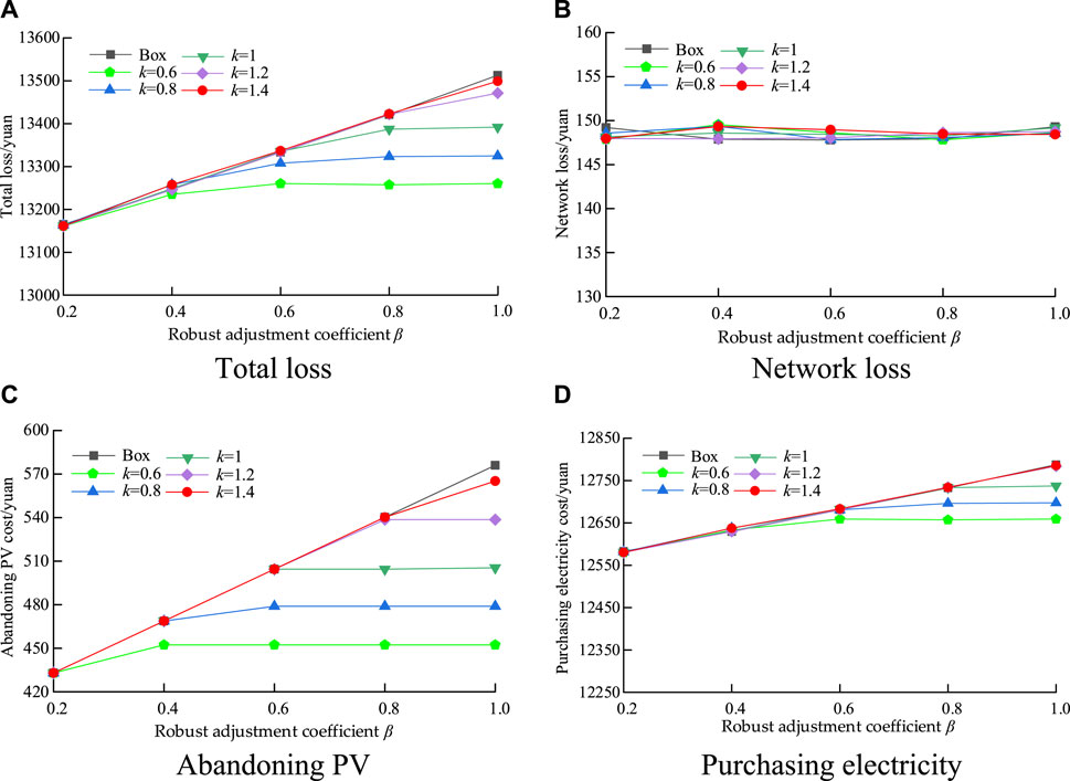
Figure 10. Impact of the robust adjustment coefficient $\beta$ on various costs: (A) total loss, (B) network loss, (C) abandoning PV, and (D) purchasing electricity.

The robustness of the constructed polyhedral set is determined by the robustness adjustment coefficient $\beta$. When the robust adjustment coefficient $\beta$ is small, the adaptability of the system to distributed PV disturbance is poor, and the cost of PV abandonment is almost unchanged whether the box set or the convex hull polyhedral set is used. On the contrary, when the robust adjustment coefficient $\beta$ is larger, the system has better adaptability to distributed PV disturbance. Therefore, for the robust adjustment coefficient $\beta =1$, the use of box sets cannot accurately respond to various situations in PV generation, which may lead to higher PV abandonment costs. However, when the convex hull polyhedral set is used, the envelope range of the convex hull set will be different due to different scaling factors k. When the scaling factor $k=0.6$, the envelope range of the convex hull polyhedral set is also small. In this case, changing the size of the robust adjustment coefficient $\beta$ does not significantly affect the cost of PV abandonment. However, when the scaling factor $k=1.4$, the convex hull uncertainty set will encompass all the historical data, so the corresponding adjustment will be made according to the increase in the robust adjustment coefficient $\beta$, which will affect the PV abandonment cost. The change trend of the cost of purchasing electricity is similar to the cost of abandoning PV. When the scaling factor $k>1$, the convex hull uncertain set covers all the worst historical scenarios as well as the box set. In this case, in order to stabilize the system power balance, the system needs to filter most of the uncertain PV injection and increase the gateway power. However, when the scaling factor $k\le 1$, the convex hull uncertain set cannot completely encompass all the historical data, and some of the worst scenarios may be missed. Similar to the cost of abandoning PV, the cost of purchasing electricity may remain the same despite changing the size of the robust adjustment coefficient $\beta$.

5.2.3 The various costs of the three polyhedral set-based robust optimization methods

The influences of the three polyhedral set-based RO methods on various costs are further compared, as shown in Table 3. It can be seen from Table 3 that when different polyhedral set-based RO methods are adopted, the cost of the hyperplane polyhedral set-based RO method is lower than that of the convex hull polyhedral set-based RO method and the box set-based RO method, except that the system network loss is basically unchanged. The convex hull polyhedral set-based RO method needs to scale the original convex hull to achieve the purpose of enveloping all historical data. Figure 3 shows that when the scaling factor $k=1.4$, the convex hull uncertainty set envelopes all historical data on the PV output. Although this enhances the robustness of the solution results, an excessive scale of data for some scenarios increases the conservatism of the solution, making the total cost of the convex hull polyhedral set-based RO method close to the box set-based RO method. The hyperplane polyhedral set-based RO method uses the mathematical idea of a hyperplane to greatly reduce the envelope range, optimize the robustness of the system, and reduce the conservatism of the system on the basis of enveloping all the historical data on PV. Therefore, the distributed PV system, using the hyperplane polyhedral set-based RO method, reduces the cost of PV abandonment and electricity purchase. It can be seen that the hyperplane polyhedral set-based RO method not only optimizes the robustness of the result but also reduces its conservatism.

Table 3

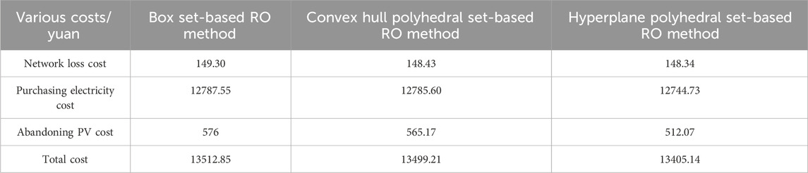
Table 3. Impact of three uncertain set-based RO methods on various costs.

5.2.4 The voltage distribution under three uncertain set-based RO methods

Figure 11 shows the node voltage distribution of the improved IEEE-33 bus system for the box set-based RO method with the robust adjustment coefficient $\beta =1$, the convex hull polyhedral set-based RO method with a scaling factor $k=1.4$, and the hyperplane polyhedral set-based RO method. Figure 11 shows that the voltages of the three uncertain set-based RO methods are all distributed in the range of 0.95 p.u.∼1.05 p.u. However, during the distributed PV generation period (10:00–14:00), the node voltage using the box set-based RO method is higher than that of the other two set-based RO methods. The node voltage of the hyperplane polyhedral set-based RO method is generally stable, and the voltage fluctuation is less than that of the convex hull polyhedral set-based RO method. This further shows that the hyperplane polyhedral set-based RO method has stronger robustness and better conservation compared to the convex hull polyhedron set-based RO method.

Figure 11

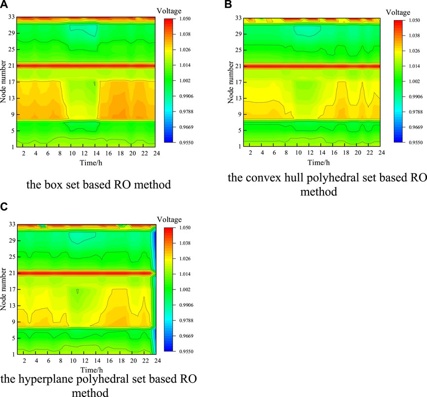
Figure 11. Node voltage distribution under three uncertain set-based RO methods: (A) box set-based RO method, (B) convex hull polyhedral set-based RO method, and (C) hyperplane polyhedral set-based RO method.

6 Conclusion

In this paper, a new distribution system robust dispatching model based on adaptive data-driven polyhedral sets is constructed and solved using the C&CG algorithm. Finally, by comparing three new distribution system robust dispatching methods based on polyhedral sets, the simulation results show the following:

(1) When the robust adjustment coefficients are the same, the total cost of the system using the convex hull polyhedral set-based RO method is lower than that using the box set-based RO method. For the convex hull polyhedral set-based RO method with different scaling factors, the robustness of the optimization results can be enhanced by expanding the scaling factors.

(2) Compared with the box set-based RO and convex hull polyhedral set-based RO methods, the hyperplane polyhedral set-based RO method using adaptive data-driven polyhedral sets can describe the distribution range of uncertain variables more accurately, and reduce the envelope of the low-probability blank region and the conservatism of optimization results. Therefore, compared with the convex hull polyhedral set-based RO method, the new robust dispatching method based on the adaptive data-driven hyperplane polyhedral set-based RO method has lower conservatism and stronger robustness.

Due to the main research direction of this paper being the impact of the uncertainty of photovoltaic output fluctuations on the distribution network, the main control mode of the photovoltaic model in this paper is the hybrid control mode. The grid-type control can only operate in parallel to the grid and cannot operate independently. It is synchronized by extracting the reference voltage phase angle through phase detection links, such as the phase-locked loop (PLL). The grid-type control is synchronized by generating phase angles through power control (Zhang et al., 2010; Harnefors et al., 2022; Xiao et al., 2023a; Xiao et al., 2023b). Therefore, from the perspective of control modes, all three types of control will have a certain impact on the power flow of the distribution network:

1. Photovoltaic grid-type: This type of system is mainly responsible for supplying local loads, and the power flow is mainly limited within the photovoltaic power generation system.

2. Grid following: When the electricity generated by the photovoltaic power generation system exceeds the local load demand, the excess energy will be transmitted to other places through the grid, leading to adjustments in the distribution of power flow in the grid.

3. Hybrid control: Hybrid control combines photovoltaic power generation systems with other energy systems and coordinates management through intelligent control strategies. This connection method can achieve complementarity and balance among various energy systems, thereby affecting the power flow distribution of the power system. For example, when photovoltaic power generation is insufficient or unable to generate electricity at night, other energy systems (such as wind power generation, energy storage systems, etc.) can supplement power supply and adjust the distribution of power flow.

In order to further study the impact of photovoltaic integration on the power system, research can be conducted from the perspectives of photovoltaic fluctuation uncertainty and different control modes of photovoltaic systems. Future research will focus on different photovoltaic control modes, as mentioned above, such as grid-following control and grid-forming control of photovoltaic systems. When there is fluctuation in the connected photovoltaic system, the operating results of the power system will change. In addition, it is necessary to consider factors such as how the reactive power of the system changes and how to maintain the system voltage stability when a large amount of photovoltaic energy is injected into the distribution network (Mehrdad et al., 2020).

Data availability statement

The original contributions presented in the study are included in the article/Supplementary Material; further inquiries can be directed to the corresponding author.

Author contributions

YY: data curation and writing–review and editing. JW: software and writing–original draft. DP: formal analysis and writing–review and editing. JZ: project administration and writing–original draft. FL: investigation and writing–original draft. XY: methodology and writing–original draft.

Funding

The author(s) declare that no financial support was received for the research, authorship, and/or publication of this article.

Conflict of interest

Authors YY, JW, and DP were employed by the Electric Power Research Institute of Guizhou Power Grid Co., Ltd. Author FL was employed by China Southern Power Grid Digital Power Grid Group Co., Ltd.

The remaining authors declare that the research was conducted in the absence of any commercial or financial relationships that could be construed as a potential conflict of interest.

Publisher’s note

All claims expressed in this article are solely those of the authors and do not necessarily represent those of their affiliated organizations, or those of the publisher, the editors, and the reviewers. Any product that may be evaluated in this article, or claim that may be made by its manufacturer, is not guaranteed or endorsed by the publisher.

References

Abad, M., and Ma, J. (2021). Photovoltaic hosting capacity sensitivity to active distribution network management. IEEE Trans. Power Syst. 36, 107–117. doi:10.1109/tpwrs.2020.3007997

CrossRef Full Text | Google Scholar

Abad, M., Seydali, S., Ma, J., Zhang, D., Ahmadyar, A., and Shabir, M. H. (2018). Probabilistic assessment of hosting capacity in radial distribution systems. IEEE Trans. Sustain. Energy 9 (4), 1935–1947. doi:10.1109/tste.2018.2819201

CrossRef Full Text | Google Scholar

Aenovi, R., and Jakus, D. (2020). Maximization of distribution network hosting capacity through optimal grid reconfiguration and distributed generation capacity allocation/control. Energies 13, 5315–5330. doi:10.3390/en13205315

CrossRef Full Text | Google Scholar

Capitanescu, F., Florin, O., Luis F, M., Harag, H., and Nikos, D. (2015). Assessing the potential of network reconfiguration to improve distributed generation hosting capacity in active distribution systems. IEEE Trans. Power Syst. A Publ. Power Eng. Soc. 30 (1), 346–356. doi:10.1109/tpwrs.2014.2320895

CrossRef Full Text | Google Scholar

Chen, X., Wu, W., and Zhang, B. (2018). Robust capacity assessment of distributed generation in unbalanced distribution networks incorporating ANM techniques. IEEE Trans. Sustain. Energy 9 (2), 651–663. doi:10.1109/tste.2017.2754421

CrossRef Full Text | Google Scholar

Chen, X., Wu, W., Zhang, B., and Lin, C. (2017). Data-driven DG capacity assessment method for active distribution networks. IEEE Trans. Power Syst. 32 (5), 3946–3957. doi:10.1109/tpwrs.2016.2633299

CrossRef Full Text | Google Scholar

Dent, C. J., Ochoa, L. F., and Harrison, G. P. (2010). Network distributed generation capacity analysis using OPF with voltage step constraints. IEEE Trans. Power Syst. 25 (1), 296–304. doi:10.1109/tpwrs.2009.2030424

CrossRef Full Text | Google Scholar

Ding, F. M. B., and Mather, B. (2017). On distributed PV hosting capacity estimation, sensitivity study, and improvement. IEEE Trans. Sustain. Energy 8 (3), 1010–1020. doi:10.1109/tste.2016.2640239

CrossRef Full Text | Google Scholar

Gao, F., Song, X., Li, J., Zhang, Y., Ma, W., and Zhang, H. (2017). DG integration capacity analysis under harmonic constraints. J. Eng. 2017, 1918–1922. doi:10.1049/joe.2017.0664

CrossRef Full Text | Google Scholar

Harnefors, L., Schweizer, M., Kukkola, J., Routimo, M., Hinkkanen, M., and Wang, X. (2022). Generic PLL-based grid-forming control. IEEE Trans. Power Electron. 37 (2), 1201–1204. doi:10.1109/TPEL.2021.3106045

CrossRef Full Text | Google Scholar

He, S., Gao, H., Tian, H., Wang, L., Liu, Y., and Liu, J. (2021). A two-stage robust optimal allocation model of distributed generation considering capacity curve and real-time price based demand response. J. Mod. Power Syst. Clean Energy 9, 114–127. doi:10.35833/mpce.2019.000174

CrossRef Full Text | Google Scholar

IsmaSmA, S. M., Sheaa, B., Aya, C., and Zobaa, A. F. (2019). State-of-the-art of hosting capacity in modern power systems with distributed generation. Renew. Energy 130, 1002–1020. doi:10.1016/j.renene.2018.07.008

CrossRef Full Text | Google Scholar

Kersting, W. H. (April 2010). A comprehensive distribution test feeder. Proceedings of the Transmission & Distribution Conference & Exposition. IEEE. New Orleans, LA, USA doi:10.1109/TDC.2010.5484418

CrossRef Full Text | Google Scholar

Leng, R., Li, Z., and Xu, Y. (2023). Two-stage stochastic programming for coordinated operation of distributed energy resources in unbalanced active distribution networks with diverse correlated uncertainties. J. Mod. Power Syst. Clean Energy 11, 120–131. doi:10.35833/mpce.2022.000510

CrossRef Full Text | Google Scholar

Masoume, M., Ahmad, A., Mahdi, S., Scott, P., and Blackhall, L. (2022). Adjustable robust approach to increase DG hosting capacity in active distribution systems. Electr. Power Syst. Res. 211, 108347. doi:10.1016/j.epsr.2022.108347

CrossRef Full Text | Google Scholar

Mehrdad, A., Amin, M., and Mohammed, H. (2020). Two-stage robust sizing and operation Co-optimization for residential PV-battery systems considering the uncertainty of PV generation and load. IEEE Trans. Industrial Inf. 17 (99), 1. doi:10.1109/TII.2020.2990682

CrossRef Full Text | Google Scholar

Moreira, S. G., Kalache, N., and Paschoareli, D. (June 2017). “Improving the hosting capacity of photovoltaic distributed generators in low voltage distribution systems by using demand response,” in Proceedings of the IEEE international conference on environment and electrical engineering and 2017 IEEE industrial and commercial power systems europe (EEEIC/I&CPS europe) (IEEE). Milan, Italy doi:10.1109/EEEIC.2017.7977753

CrossRef Full Text | Google Scholar

Palahalli, P., Maffezzoni, P., Arboleya, A., and Gruosso, G. (2022). Implementing stochastic response surface method and copula in the presence of data-driven PV source models. IEEE Trans. Sustain. Energy 13 (4), 2370–2380. doi:10.1109/tste.2022.3197893

CrossRef Full Text | Google Scholar

Qiu, H., Gu, W., Xu, X., Pan, G., Liu, P., Wu, Z., et al. (2021). A historical-correlation-driven robust optimization approach for microgrid dispatch. IEEE Trans. SMART GRID 12 (2), 1135–1148. doi:10.1109/tsg.2020.3032716

CrossRef Full Text | Google Scholar

Qiu, Y., Li, Q., Huang, L., Sun, C., Wang, T., and Chen, W. (2020). Adaptive uncertainty sets-based two-stage robust optimisation for economic dispatch of microgrid with demand response. IET Renew. Power Gener. 14, 3608–3615. doi:10.1049/iet-rpg.2020.0138

CrossRef Full Text | Google Scholar

Su, N., Wei, P., Peter, S., Alahakoon, D., and Yu, X. (2018). Optimizing rooftop photovoltaic distributed generation with battery storage for peer-to-peer energy trading. Appl. Energy 228, 2567–2580. doi:10.1016/j.apenergy.2018.07.042

CrossRef Full Text | Google Scholar

Sun, P., Luo, M. W., Sun, Z. X., Liu, T. C., Deng, C. H., Chen, L., et al. (2015). Penetration capacity analysis of distributed generation considering overcurrent relay protection and flux-coupling type FCL. Adv. Mater. Res. 1070, 923–928. doi:10.4028/www.scientific.net/amr.1070-1072.923

CrossRef Full Text | Google Scholar

Taha, H., Alham, M., and Youssef, H. (2021). Hosting capacity maximization of wind and solar DGs in distribution networks using demand response and renewables curtailment. Int. J. Energy Convers. (IRECON) 9 (3), 103. doi:10.15866/irecon.v9i3.20066

CrossRef Full Text | Google Scholar

Tan, X., Wang, Z., and Li, Q. (2020). Segmentation algorithm for maximum hosting capacity of distributed generator accessing to distribution network considering multiple constraints. Automation Electr. Power Syst., 44 72–80.

Google Scholar

Torquato, R., Salles, D., Oriente, P. C., Meira, P. C., and Magalhaes, F. W. (2018). A comprehensive assessment of PV hosting capacity on low-voltage distribution systems. IEEE Trans. Power Deliv. 33 (2), 1002–1012. doi:10.1109/tpwrd.2018.2798707

CrossRef Full Text | Google Scholar

Wang, B., Zhang, C., Dong, Z., and Li, X. (2021). Improving hosting capacity of unbalanced distribution networks via robust allocation of battery energy storage systems. IEEE Trans. Power Syst. 36 (3), 2174–2185. doi:10.1109/tpwrs.2020.3029532

CrossRef Full Text | Google Scholar

Wang, S., Chen, S., and GeL Wu, L. (2016). Distributed generation hosting capacity evaluation for distribution systems considering the robust optimal operation of OLTC and SVC. IEEE Trans. Sustain. energy 7 (3), 1111–1123. doi:10.1109/tste.2016.2529627

CrossRef Full Text | Google Scholar

Wu, H., Yuan, Y., Zhu, J., Qian, K., and Xu, Y. (2019). Potential assessment of spatial correlation to improve maximum distributed PV hosting capacity of distribution networks. J. Mod. Power Syst. Clean Energy 9, 800–810. doi:10.35833/mpce.2020.000886

CrossRef Full Text | Google Scholar

Xiao, H., Gan, H., Yang, P., Li, L., Hao, Q., et al. (2023). Robust submodule fault management in modular multilevel converters with nearest level modulation for uninterrupted power transmission. IEEE Trans. Power Del, 1–16. doi:10.1109/TPWRD.2023.3343693

CrossRef Full Text | Google Scholar

Xiao, H., He, H., Zhang, L., and Liu, T. (2023). Adaptive grid-synchronization based grid-forming control for voltage source converters. IEEE Trans. Power Syst., 1–4. doi:10.1109/TPWRS.2023.3338967

CrossRef Full Text | Google Scholar

Xu, G., Zhang, B., and Zhang, G. (2021). Distributed and robust optimal scheduling model for large-scale electric vehicles connected to grid. Trans. China Electrotech. Soc., 36 565–578.

Google Scholar

Yu, D., Yang, M., and Zhai, H. (2016). Review of application research on robust optimization in power system dispatching decision. Power Syst. Autom. 40 (07), 134–143+148.

Google Scholar

Zeng, B., and Zhao, L. (2013). Solving two-stage robust optimization problems using a column-and-constraint generation method. Operations Res. Lett. 41, 457–461. doi:10.1016/j.orl.2013.05.003

CrossRef Full Text | Google Scholar

Zhang, L., Harnefors, L., and Nee, H.-P. (2010). Power-synchronization control of grid-connected voltage-source converters. IEEE Trans. Power Syst. 25 (2), 809–820. doi:10.1109/tpwrs.2009.2032231

CrossRef Full Text | Google Scholar

Zhang, S., Fang, Y., Zhang, H., Cheng, H., and Wang, X. (2022). Maximum hosting capacity of photovoltaic generation in SOP-based power distribution network integrated with electric vehicles. IEEE Trans. Industrial Inf. 18 (11), 8213–8224. doi:10.1109/tii.2022.3140870

CrossRef Full Text | Google Scholar

Zhang, X., Yao, L., and Chen, C. (2022). A novel two-stage robust model for co-optimization of reconfiguration and reactive power in AC/DC hybrid distribution network. Power Syst. Technol., 46 1149–1162.

Google Scholar