An integrated energy system day-ahead scheduling method based on an improved dynamic time warping algorithm

1 Introduction

The global energy shortage and environmental issues are pressing challenges for the world, necessitating an accelerated shift toward green and low-carbon energy transformation and the rapid development of new industries (Antonazzi et al., 2023). The integration of renewable energy on a large scale has led to the need for an integrated energy system (IES) that combines various energy sources, such as wind, solar, and chemical energy, within a region in an effective way to promote the utilization and development of new energy systems (Martínez Ceseña et al., 2020). However, the uncertainty of new energy output at the source end and energy consumption at the load end increases the volatility of IES, impacting the accuracy of its day-ahead scheduling scheme (Jena et al., 2022). Therefore, studying the IES day-ahead scheduling method becomes crucial in the face of growing uncertainty.

Currently, two methods are prevalent for addressing uncertainties in the IES: i) the probabilistic form and ii) the non-probabilistic form. The former accurately describes uncertainty, while the latter, comprising robust and interval methods, has a simpler modeling structure. Kalim et al. (2021) predicted the behavior of wind and light renewable energy using probability and cumulative density functions, and they solved the smart microgrid model based on the multi-objective wind-driven optimization (MOWDO) algorithm and multi-objective genetic algorithm by Pareto criterion and fuzzy mechanism using the demand–response scenario and tilt block tariff as the scenarios to optimize the operating cost, pollution emission, and system availability at the same time. Meanwhile, Sajjad et al. (2022) further developed a responsive consumer model based on the demand response of Kalim et al. (2021) and a multi-objective dispatch model based on MOWDO to optimize the operating cost, curtailable load reduction cost, pollution emission, transferable load, and wind power generation. Hengyu et al. (2023) proposed a thermoelectric coupled probability multi-energy flow calculation method establishing the probabilistic and correlation models. Ran et al. (2024) constructed an optimization model considering load probability uncertainty based on easily accessible conditional risk values. Representing uncertainties through probability functions demands extensive historical data, making it challenging to obtain accurate distributions. To enhance accuracy, Liu et al. (2023) used kernel density estimation to obtain probability density distributions of wind speed, solar radiation, and multidemand, and typical scenarios are generated using Latin hypercube sampling and self-organizing mapping. Duan et al. (2023) generated typical daily output scenarios of the scenery using the Frank-copula theory with joint probability distributions for source load uncertainty. Xu et al. (2023) used Monte Carlo simulation and K-means clustering methods to generate typical scenarios and attempted to minimize the operating costs using an adaptive differential evolutionary algorithm based on the success history.

Despite improvements in accuracy, generating typical scenarios affects the robustness of IES scheduling. Hafeez et al. (2020) actively participated in the market through demand response programs to cope with load uncertainty and proposed wind-driven bacterial foraging algorithms to solve energy management strategies based on price-based demand response programs. Ghulam et al. (2020) established an integrated framework based on artificial neural networks (ANNs) and the gray wolf modified enhanced differential evolution (GmEDE) algorithm to improve the efficient energy management of residential buildings by predicting price-based demand response signals and energy consumption through ANNs and efficiently managing residential buildings under the predicted values through GmEDE. Ahmad et al. (2023) developed a real-time energy optimization algorithm based on the framework of Lyapunov optimization. Li et al. (2023) considered the integrated demand response and inertia of various energy sources to construct a robust optimization model, achieving optimality under worst-case scenarios. Ma et al. (2022) developed a model of an integrated electricity–gas–heat system at the user level, which is solved using a decentralized, robust algorithm to protect the security and privacy of the various participants in the system. Interval variables encompassing more information and handling unknown distribution parameters offer an alternative (Xiong et al., 2023). Gong et al. (2020) proposed a dynamic interval multi-objective co-evolutionary optimization framework based on interval similarity to solve dynamic interval multi-objective optimization problems and adopted a response strategy to quickly track the changing Pareto frontiers of the optimization problem. Zhang et al. (2023) dealt with the uncertainty issues of wind energy using interval numbers to model wind energy, and an interval-based optimization scheduling model was established to minimize operating costs. However, relying solely on upper and lower bounds neglects correlations, which results in conservative outcomes. To address conservatism, Zheng et al. (2022) introduced a noise element variable through an affine algorithm, formulating an interval affine optimization scheduling model for multi-microgrids. Nevertheless, this study only evaluates the approach based on forecasting data and lacks solutions for all possible scenarios.

Table 1 compares the aforementioned uncertainty modeling methods and analyzes their strengths and weaknesses.

Table 1

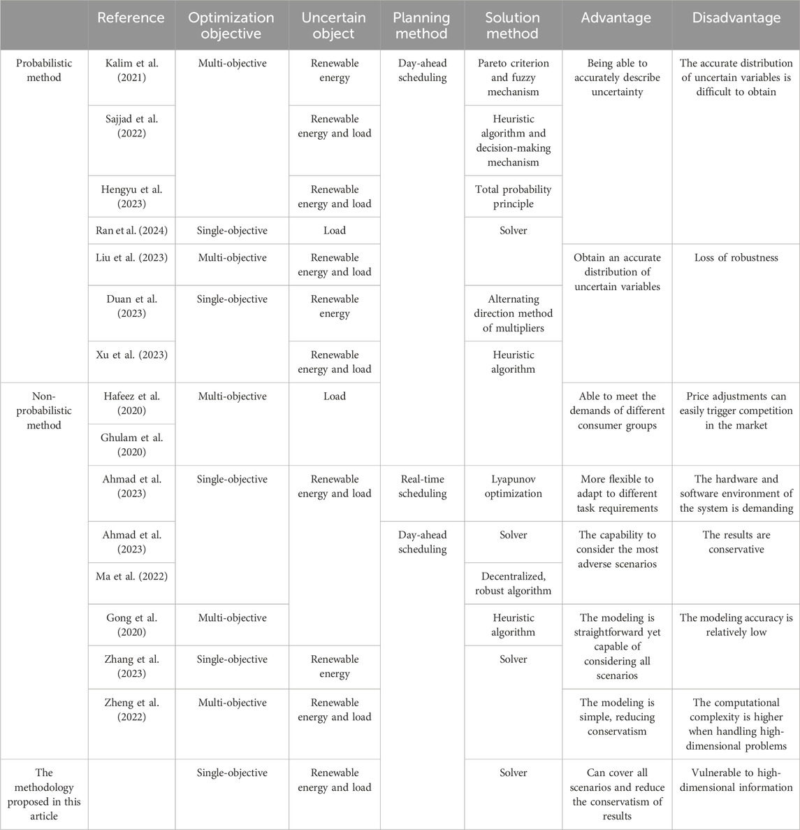
Table 1. Comparison of different uncertainty modeling methods.

Unlike k-means clustering, hierarchical clustering does not require a prior specification of clusters but relies on data point similarity. Traditional similarity measures like the Euclidean distance method, though computationally simple, face challenges in recognizing data shape deformations and requiring equal-length time-series data (Ezugwu et al., 2022). The dynamic time warping (DTW) algorithm, known for addressing shape deformations and unequal time-series data (Holder et al., 2023), has been introduced in power system analysis (Gunawan and Huang, 2021; Shuai et al., 2023). However, due to the high-dimensional nonlinear characteristics of the IES source and load data, direct clustering calculations can be complex (Liu and Chen, 2019).

Building upon existing research, this paper emphasizes the advantages of DTW in addressing conservative scheduling issues in the IES. However, few studies focus on IES scheduling schemes under all possible scenarios and provide references for scheduling personnel. To address this, the paper preprocesses IES source and load data, converting high-dimensional nonlinear data into low-dimensional linear interval data. An enhanced DTW is then employed for hierarchical clustering, followed by the establishment of a day-ahead interval affine scheduling model based on economic factors and correlations. The resulting scheduling scheme provides intervals for all typical scenarios, offering valuable references for dispatchers and elucidating the fluctuation range and operational interval of the IES. The primary contributions include the following:

(1) Establishing an IES day-ahead scheduling model considering economic factors and the correlation of uncertain variables.

(2) Improving the original DTW using the interval distance formula and applying it to measure the similarity of linear interval data obtained through dimensionality reduction.

(3) Presenting a scheduling scheme for all typical scenarios, providing a reference for dispatchers, and clarifying the fluctuation range and operational interval of the IES.

2 Integrated energy system structure and model

2.1 Integrated energy system model

The park-integrated electrical heating systems (PIEHSs) discussed in this article are illustrated in Figure 1, comprising two main components: the power subsystem and the thermal subsystem. The PIEHS source side incorporates the superior power grid, gas grid, wind turbine (WT), and photovoltaic (PV). The system coupling side equipment includes combined heat and power (CHP) and an electric boiler (EB). The PIEHS load side includes electrical and thermal loads. The system’s energy storage process encompasses electric energy storage (EES) and thermal energy storage (TES).

Figure 1

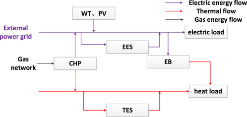
Figure 1. PIEHS structure diagram.

2.2 Modeling of uncertain variables

Various factors, including weather changes and consumer psychology, lead to fluctuations in wind and solar power output and load demand. Although existing research suggests that these fluctuations follow probability distributions, obtaining accurate probability density functions during actual operation is challenging (Yang et al., 2023). However, obtaining the value range of uncertain quantities from historical data is relatively straightforward and helps avoid the interference of prediction errors. Therefore, this article models wind and solar power output and load demand using interval numbers based on historical data (Bai et al., 2016).

$\left[P_t^{\text{pv}}\right]=\left[{\underset{\_}{P}}^{\text{pv}},{\overline{P}}^{\text{pv}}\right],(1)$

$\left[P_t^{wt}\right]=\left[{\underset{\_}{P}}^{wt},{\overline{P}}^{wt}\right],(2)$

$\left[P_t^{\text{load}}\right]=\left[{\underset{\_}{P}}^{\text{lood}},{\overline{P}}^{load}\right],(3)$

where $\left[P_t^{\text{pv}}\right]$ and ${\underset{\_}{P}}^{\text{pv}}$ are the output ranges of photovoltaic and wind turbines at time t, respectively; ${\overline{P}}^{\text{pv}}$ and $\left[P_t^{wt}\right]$ are the upper and lower limits of the photovoltaic output, respectively; ${\underset{\_}{P}}^{wt}$ and ${\overline{P}}^{wt}$ are the upper and lower limits of the wind turbine output, respectively; $\left[P_t^{\text{load}}\right]$ is the load demand range at time t; and ${\underset{\_}{P}}^{\text{lood}}$ and ${\overline{P}}^{load}$ are the limits of the load demand range.

2.3 PIEHS equipment model

2.3.1 CHP unit model

The CHP unit, a key component in the electric heating system, is assumed to operate in a “heat-to-power” mode in this article. The CHP unit model is as follows (Yansong et al., 2023):

$\left\{\begin{array}{l}{P}_{\text{CHP}}^t={\eta }_{\mathrm{E}}{G}_{\text{CHP}}^t\\ H_{\text{CHP}}^t={\eta }_S{\eta }_{\mathrm{H}}{G}_{\text{CHP}}^t\end{array}\right.,(4)$

where $P_{\text{CHP}}^t$ and $H_{\text{CHP}}^t$ are the electrical and thermal power output of the CHP unit at time t, respectively; $G_{\text{CHP}}^t$ is the power of natural gas consumed by the CHP unit at time t; ${\eta }_{\mathrm{E}}$ and ${\eta }_S$ are the electrical and thermal efficiencies of the CHP unit, respectively. ${\eta }_{\mathrm{H}}$ is the CHP unit heat recovery efficiency.

The constraints are as follows:

$\left\{\begin{array}{c}-\Delta P_{\text{CHP}}^{\text{down}}\left(t\right)\le P\left(t\right)-P\left(t-1\right)\le \Delta P_{\text{CHP}}^{\text{up}}\left(t\right)\\ -\Delta Q_{\text{CHP}}^{\text{down}}\left(t\right)\le Q\left(t\right)-Q\left(t-1\right)\le \Delta Q_{\text{CHP}}^{\text{up}}\left(t\right)\end{array}\right..(5)$

$P_{CHP,\min }\le p_{CHP,t}\le P_{CHP,\max }.(6)$

In the above formula, $\Delta P_{\text{CHP}}^{\text{down}}\left(t\right)$ and $\Delta P_{\text{CHP}}^{\text{up}}\left(t\right)$ are the maximum downhill and uphill rates of the electric output of the CHP unit at time t, respectively; $\Delta Q_{\text{CHP}}^{\text{down}}\left(t\right)$ and $\Delta Q_{\text{CHP}}^{\text{up}}\left(t\right)$ are the maximum downhill and uphill rates of the thermal output of the CHP unit at time t, respectively; $p_{CHP,t}$ is the thermal output of the CHP unit at time t; and $P_{CHP,\min }$ and $P_{CHP,\max }$ are the minimum and maximum thermal output values of the CHP unit, respectively.

2.3.2 EB model

The EB, acting as a coupling device between electric heating systems, follows the model given below:

$P_{\alpha ,i}=\left(1-{\delta }_i\right)P_{\alpha -1,i}+\left({\eta }_{cha,i}{P}_{cha,\alpha ,i}-\frac{P_{dis,\alpha ,i}}{{\eta }_{dis,i}}\right)\Delta \alpha i\in E,T,(7)$

where $Q_{EB,t}$ is the efficiency of the electricity-to-heat conversion, ${\eta }_{EB}$ is the absorbed electric power at time t, and $P_{EB,t}$ is the emitted thermal power at time t.

The constraints are as follows:

$-R_{EB,t}^{\text{down}}\le Q_{EB,t}-Q_{EB,t-1}\le R_{EB,t}^{\text{up}},(8)$

$Q_{EB,\min }\le Q_{EB,t}\le Q_{EB,\max },(9)$

where $R_{EB,t}^{\text{down}}$ and $R_{EB,t}^{\text{up}}$ are the maximum values of the downhill and uphill speed of the EB, respectively, and $Q_{EB,\min }$ and $Q_{EB,\max }$ are the minimum and maximum values of the thermal power output of the EB, respectively.

2.3.3 Energy storage model

Energy storage in PIEHS involves ESS and TES, and its model is outlined as follows:

$P_{\alpha ,i}=\left(1-{\delta }_i\right)P_{\alpha -1,i}+\left({\eta }_{cha,i}{P}_{cha,\alpha ,i}-\frac{P_{\text{dis},\alpha ,i}}{{\eta }_{dis,i}}\right)\Delta \alpha i\in E,T,(10)$

where $P_{\alpha ,i}$ is the stored energy of the energy storage device i within time t; ${\delta }_i$ is the dissipation rate of the energy storage device i; ${\eta }_{cha,i}$ is the charging efficiency of the energy storage device i; $P_{cha,\alpha ,i}$ is the input of the energy storage device i within time t; ${\eta }_{dis,i}$ is the discharge efficiency of the energy storage device i; $P_{\text{dis},\alpha ,i}$ is the output of the energy storage device i within time t; $\Delta \alpha$ is the time interval between two actions; and $i\in E,T$ is an electrical energy storage device or a thermal energy storage device.

The constraints are as follows:

$\left\{\begin{array}{l}{N}_{i,\min }\le N_{i,t}\le N_{i,\max }\\ 0\le P_{cha,i,t}\le P_{cha,i,\max }{B}_{cha,i}^t\\ 0\le P_{dis,i,t}\le P_{dia,i,\max }{B}_{dis,i}^t\\ B_{cha,i}^t+B_{dis,i}^t=1\\ N_{i,t}=N_{i,0}\end{array}\right.i\in E,T,(11)$

where $N_{i,\min }$ is the minimum capacity of the energy storage device i; $N_{i,t}$ is the state of the energy storage device i at time t; $N_{i,\max }$ is the maximum capacity of the energy storage device i; $P_{cha,i,t}$ is the charging power of the energy storage device i at time t; $P_{cha,i,\max }$ is the maximum charging power of the energy storage device i; $P_{dis,i,t}$ is the discharging power of the energy storage device i at time t; $P_{dia,i,\max }$ is the maximum discharging power of the energy storage device i; $B_{cha,i}^t$ and $B_{dis,i}^t$, respectively, represent the charging and discharging states of the energy storage device i at time t, which are 0–1 variables; and $N_{i,0}$ is the initial capacity of the energy storage device i.

3 Hierarchical clustering based on improved dynamic time warping

In the daily scheduling of the IES, most scheduling schemes are typically based on the forecast data of wind, light, and loads. However, such schemes are specific to particular scenarios and do not account for all situations. To address this, the article clusters historical data to obtain typical scenarios and provides interval scheduling schemes for each scenario. During day-ahead dispatching, the forecast values of wind and rain load are matched with the corresponding typical scenario, offering a dispatching scheme for the dispatcher’s reference. Unlike k-means clustering, hierarchical clustering does not require setting the number of clusters in advance, resulting in more accurate clustering results. The article employs the condensed hierarchical clustering method for historical data on wind, solar power, and load, merging the closest samples and repeating the clustering process until the end threshold condition is met.

3.1 Improved dynamic time warping

When measuring the similarity of historical data, issues like data loss may arise due to malfunctions in data collection equipment, leading to unequal lengths between historical datasets. DTW enables “one-to-many” matching in uncertain variable historical data, addressing data loss issues and equalizing time-series data lengths. DTW is shown in Figure 2:

Figure 2

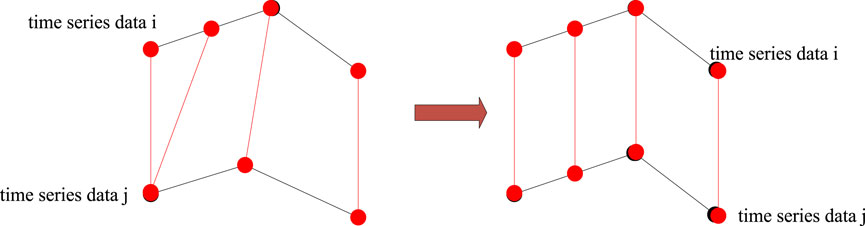
Figure 2. Schematic of DTW

3.1.1 Data preprocessing

Due to the high-dimensional and nonlinear characteristics of historical data on wind, solar, and load, direct clustering operations can pose challenges such as algorithmic time and space complexity (Liu and Chen, 2019). Therefore, historical data need to undergo preprocessing. Approximate piecewise linearization and normalization (Santiago et al., 2020) are employed for processing, reducing the dimensionality of high-dimensional data and linearizing historical data. Using a 15-min time period, the maximum and minimum values within each period form the upper and lower limits of the interval. The upper and lower limits of the subsequent periods are sequentially connected, as illustrated in Figure 3. This transforms historical data on wind, solar, and load into interval time-series data, as follows:

$\left[{P_t^{cate}}^{\prime }\right]=\left\{\left({t_X}^{\prime }+\Delta t^{\prime },\left[{P_{U1}}^{\prime },{P_{L1}}^{\prime }\right]\right),\left({t_X}^{\prime }+2\Delta t^{\prime },\left[{P_{U2}}^{\prime },{P_{L2}}^{\prime }\right]\right),\dots ,\left({t_X}^{\prime }+n\Delta t^{\prime },\left[{P_{Un}}^{\prime },{P_{\mathit{Ln}}}^{\prime }\right]\right)\right\},(12)$

${P_{Ui}}^{\prime }=\frac{P_{Ui}-\min \left\{P_{U1},P_{U2},\dots ,P_{Un}\right\}}{\max \left\{P_{L1},P_{L2},\dots ,P_{\mathit{Ln}}\right\}-\min \left\{P_{U1},P_{U2},\dots ,P_{Un}\right\}},(13)$

$P_{Li}^{\prime }=\frac{P_{Li}-\min \left\{P_{U1},P_{U2},\dots ,P_{Un}\right\}}{\max \left\{P_{L1},P_{L2},\dots ,P_{\mathit{Ln}}\right\}-\min \left\{P_{U1},P_{U2},\dots ,{P_{Un}}_n\right\}},(14)$

$\left\{\begin{array}{l}\Delta t^{\prime }=\frac{1}{n-1}\\ {t_X}^{\prime }=-\Delta t^{\prime }\end{array}\right.,(15)$

Figure 3

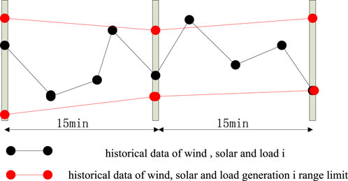
Figure 3. Preprocessing of historical data of wind, solar, and load.

where $\Delta t^{\prime }$ is the normalized time interval; $n$ is the number of time intervals; ${t_X}^{\prime }$ is the normalized time point; $\left[{P_t^{cate}}^{\prime }\right]$ is the normalized wind, solar, and load interval data, $cate\in wt、pv、load$; and ${P_{Ui}}^{\prime }$ and $P_{Li}^{\prime }$ are the normalized upper and lower limits of the time interval data, respectively.

3.1.2 Similarity measure

Eq. 12 demonstrates the transformation of wind, light, and load data into interval time-series data after preprocessing. Calculating the distance between interval data is challenging, leading to the introduction of triangular filling, as shown in Figure 4. By comparing preprocessed data along the time axis, when $t_b-t_a>t_d-t_c$, point A connects to point D, forming a triangle with points B and C. The triangle’s center of gravity and circumscribed circle radius convert the interval time-series data into a set of triplet data. Initially, the DTW method used the Euclidean distance to calculate the similarity between uncertain variables. However, the Euclidean distance fails to capture all information within uncertain variable interval data. Tran and Duckstein (2002) introduced a new formula for calculating distance based on the midpoint and radius of intervals, which can be considered a generalization of the Euclidean distance:

$D^2\left(A,B\right)={\left[\left(\frac{a_1+a_2}{2}\right)-\left(\frac{b_1+b_2}{2}\right)\right]}^2+\frac{1}{3}\left[{\left(\frac{a_1-a_2}{2}\right)}^2+{\left(\frac{b_2-b_1}{2}\right)}^2\right],(16)$

Figure 4

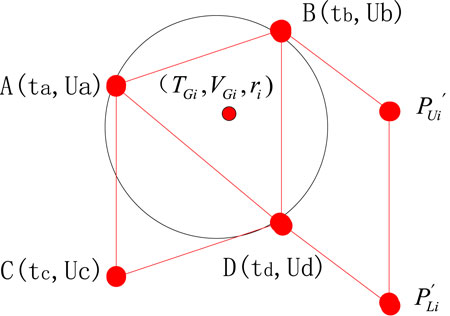
Figure 4. Interval data triangular filling.

where A and B are interval numbers in the ranges ($a_1$, $a_2$) and ($b_1$, $b_2$), respectively; $\frac{a_1+a_2}{2}$ and $\frac{b_1+b_2}{2}$ are the midpoints of A and B, respectively; and $\frac{a_1-a_2}{2}$ and $\frac{b_2-b_1}{2}$ are the radiis of A and B, respectively.

According to Equation 16, after filling the triangular interval data for $\left(T_{Gi},V_{Gi},r_i\right)$ and $\left(S_{Gi},U_{Gi},R_i\right)$, the formula for measuring the distance between them is as follows:

$d_{DTW}=\sqrt{{\left(T_{Gi}-S_{Gi}\right)}^2+{\left(V_{Gi}-U_{Gi}\right)}^2+\frac{1}{3}{\left(r_i+R_i\right)}^2}.(17)$

In the above formula, $\left(T_{Gi},V_{Gi}\right)$ and $\left(S_{Gi}-U_{Gi}\right)$ are the coordinates of the center of gravity of the ith triangle of the same uncertain quantity in $\left[{P_t^{cate}}^{\prime }\right]$; $r_i$ and $R_i$ are the outer radii of the ith triangle of the two sets of interval data.

As an example, assuming that the filled points of triangle ACD in Figure 4 are denoted as point X and the filled points of triangle ABD in Figure 4 are denoted as point Y, the sequence of points X is (1, 2, 3) and the sequence of points Y is (3, 6, 9). The distance between X and Y is as follows:

$d_{DTW}\left(XY\right)=\sqrt{{\left(1-3\right)}^2+{\left(2-6\right)}^2+\frac{1}{3}{\left(3+9\right)}^2}=8.2462.$

The distance between X and Y can be obtained by substituting the centroid coordinates (1, 2) and (3, 6) along with the radii 3 and 9 into Eq. 17. The distance between X and Y is calculated to be 8.2462.

A distance matrix of order $m\times n$ is obtained using Equation 17. The distance matrix is as follows:

$D_{m\times n}=\left(\begin{array}{ccc}{D}_{11}& \dots & D_{1n}\\ ⋮& \ddots & ⋮\\ D_{m1}& \cdots & D_{mn}\end{array}\right),(18)$

where $D_{mn}$ represents the distance between the mth data and nth data in any two sets of data under the same uncertainty in $\left[{P_t^{cate}}^{\prime }\right]$.

Next, the optimal path—the minimum-distance route from $D_{11}$ to $D_{12}$ within the distance matrix $D_{21}$—must be identified. The path selection must satisfy the following conditions:

(1) Boundary conditions: the selected path must commence from $D_{11}$ and terminate at $D_{mn}$.

(2) Monotonicity condition: the selected path must proceed monotonically over time.

(3) Continuity condition: the selected path must be contiguous, without cross-point matching.

Starting from $D_{11}$, there are three possible directions: to the right ($D_{12}$), below ($D_{21}$), and to the lower right ($D_{22}$). The smallest value among these three is chosen and continued in this manner until $D_{mn}$. The elements in the path selection are denoted as $M{D}_I\left(I\in \left[1,m+n-1\right]\right)$. The similarity measure between two sets of data under the same uncertainty can be represented as follows:

$D_{DTW}=\min {\displaystyle \sum _{I=1}^{m+n-1}}M{D}_I.(19)$

Eq. 19 indicates that the distance between two sets of data under the same uncertainty is the minimum accumulated distance.

3.1.3 Evaluation indicators

To verify the clustering effect, the sum of squared errors (SSEs) (Shang et al., 2021), Davies–Bouldin index (DBI), and Dunn validity index (DVI) (Kan et al., 2019) are used as evaluation metrics.

The SSE expression is as follows:

$SSE={\displaystyle \sum _{i=1}^n}{\displaystyle \sum _{x\in j_{Ci}}}\left({\left|x-C_i\right|}^2\right),(20)$

where $C_i$ represents the clustering center; $j_{Ci}$ is the clustering result corresponding to $C_i$; and $x$ is the point in the clustering result.

The DBI expression is as follows:

$DBI=\frac{1}{C}{\displaystyle \sum _{i=1}^C}\underset{j\ne i}{\max }\left(\frac{{\overline{x}}_{Ci}+{\overline{x}}_{Cj}}{{‖C_i-C_j‖}_2}\right),(21)$

where ${\overline{x}}_{Ci}$ and ${\overline{x}}_{Cj}$ are the average intra-class distance between any two classes; $C$ is the final number of clusters in the clustering; and ${‖C_i-C_j‖}_2$ is the distance between two cluster centers.

The DVI expression is as follows:

$DVI=\frac{\underset{xi\ne xj}{\min }\left(‖x{i}_{j_{Ci}}-x{j}_{j_{Ci}}‖\right)}{\underset{xi\ne xj}{\max }\left(‖x{i}_{j_{Ci}}-x{j}_{j_{Ci}}‖\right)},(22)$

where $x{i}_{j_{Ci}}$ and $x{j}_{j_{Ci}}$ are any two data points within $j_{Ci}$ and $‖x{i}_{j_{Ci}}-x{j}_{j_{Ci}}‖$ is the distance between $x{i}_{j_{Ci}}$ and $x{j}_{j_{Ci}}$.

A smaller DBI metric indicates a smaller within-class distance and a larger inter-class distance. Conversely, a larger DVI metric indicates a larger inter-class distance and a smaller within-class distance.

3.2 Typical scene generation

First, the normalized wind, solar, and load data are organized into a composite data sample set on a daily basis. After forming the distance matrix using Eq. 18, the optimal path is selected using DTW, and the distance between samples is calculated according to Eq. 19. Then, the data sample set is clustered using the agglomerative hierarchical clustering method. Agglomerative hierarchical clustering employs a bottom-up strategy, treating each object as a separate cluster and gradually merging the clusters, with the convergence criterion being that all data ultimately converge into a single class or reach a certain stopping threshold. The stopping threshold condition is determined as follows:

According to the definition of an isolation point in the literature (Laszlo, 2010), an isolated sequence $G\left(x_i\right)$ is defined as the DTW distance $D_{DTW}\left(x_i\right)$ between a data sample $x_i$ and a sample nearest to sample $x_i$ that is greater than a certain margin $Y\left(i\right)$ , i.e., $D_{DTW}\left(x_i\right)$ > $Y\left(i\right)$. Therefore, as $Y\left(i\right)$ decreases, the number of $G\left(x_i\right)$ will increase, and the increased number of $G\left(x_i\right)$ will be recorded as $\Delta G\left(x_i\right)$. $\Delta G\left(x_i\right)$ will increase and then decrease as $Y\left(i\right)$ decreases. Therefore, when $\Delta G\left(x_i\right)$ reaches its maximum value, $Y\left(i\right)$ is chosen as the stop threshold condition. The detailed flowchart is illustrated in Figure 5:

Figure 5

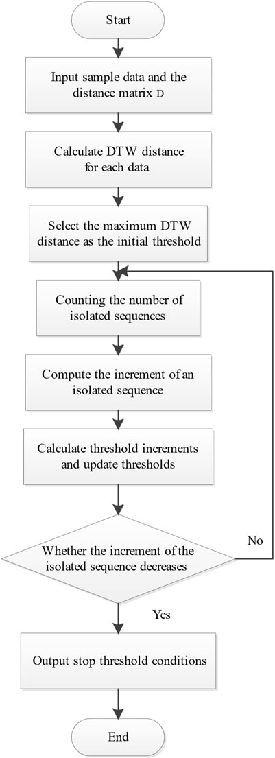
Figure 5. Generated typical scenarios.

First, the initial threshold, denoted as $D_{DTW,i}\left(x_i\right)$, is chosen as the maximum value of $D_{DTW}\left(x_i\right)$ in the entire data sample. Next, the reduction in $D_{DTW,i}\left(x_i\right)$ during cycling, denoted as $\Delta D_{DTW}\left(o\right)$, is a fractional multiple of the initial threshold, $D_{DTW,i}\left(x_i\right)=\max D_{DTW}\left(x_i\right)-\Delta D_{DTW}\left(o\right)$.The isolated sequence detection algorithm stops when the amount of $\Delta G\left(x_i\right)$ peaks, indicating a sharp increase in the number of isolated sequences produced at that threshold. Since it is necessary to compare $\Delta G\left(x_i\right)$, $\Delta G\left(x_i\right)$ is detected as the maximum at step i when $D_{DTW,i}\left(x_i\right)$ has been reduced to the same amount for the i+2nd time. The final convergence condition is, therefore, as follows: $D_{DTW}\left(stop\right)=D_{DTW,i}\left(x_i\right)+3\Delta D_{DTW}\left(o\right)$.

The final conclusion is drawn from typical scenarios. The detailed flowchart is illustrated in Figure 6.

Figure 6

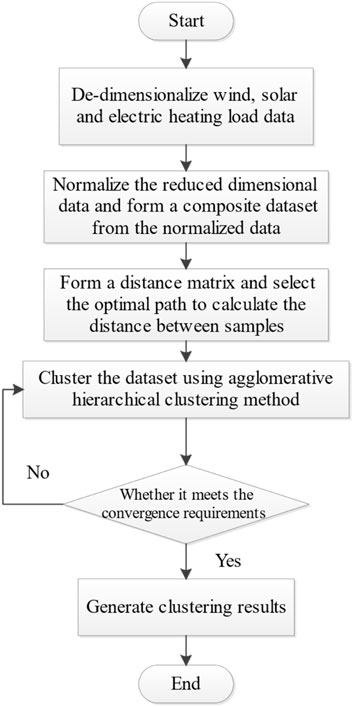
Figure 6. Clustering stopping threshold conditions.

To determine which class the predicted data belongs to, the predicted data are first pre-processed and formed into a composite data sample set according to Eqs 12–15, then the distances between the predicted data and each clustering center are calculated according to Equation 16, and finally, the predicted data are assigned to the class with the closest distance.

4 Affine-based IES interval scheduling model

4.1 Objective function

This article considers the minimum total cost of IES, comprising the sum of the operating cost of the IES equipment and the external power purchase cost, as the objective function. The objective function is as follows:

$\min F=f_1+f_2,(23)$

where $f$ is the operating cost of IES and $f_2$ is the power supply cost of IES’s superior power grid.

4.1.1 IES equipment operating cost

The operating costs of the IES equipment include WT and PV operating costs, CHP fuel costs, EB operating costs, and the operating costs of energy storage devices.

The operating costs of the equipment are as follows:

$f_1=F_{WT}+F_{PV}+F_{CHP}+F_{EB}+F_{ES},(24)$

where $F_{WT}$, $F_{PV}$, $F_{CHP}$, $F_{EB}$, and $F_{ES}$ are, respectively, the $WT$ operation cost, $PV$ operation cost, operating cost of the CHP unit, EB operation cost, and energy storage operation cost.

The operating cost of WT is as follows:

$F_{WT}={\displaystyle \sum _{t=1}^T}{\lambda }_{WT}{P}_t^{\text{wt}},(25)$

where ${\lambda }_{WT}$ is the unit WT operating cost and $P_t^{\mathrm{wt}}$ is the WT output power within the time $t$.

The operating cost of PV is as follows:

$F_{PV}={\displaystyle \sum _{t=1}^T}{\lambda }_{PV}{P}_t^{pv},(26)$

where ${\lambda }_{PV}$ is the unit PV operating cost and $P_t^{pv}$ is the PV output power within time $t$.

The operating cost of the CHP unit is as follows:

$F_{CHP}={\displaystyle \sum _{t=1}^T}{\lambda }_G{Q}_{G,t},(27)$

where ${\lambda }_G$ is the unit cost of gas purchase and $Q_{G,t}$ is the amount of gas purchased within time $t$.

The operating cost of EB is as follows:

$F_{EB}={\displaystyle \sum _{t=1}^T}{\lambda }_{EB}{P}_{EB,t},(28)$

where ${\lambda }_{EB}$ is the unit EB operating cost and $P_{EB,t}$ is the electric power absorbed within time $t$.

The operation costs of energy storage are as follows:

$F_{ES}=F_{EES}+F_{HES},(29)$

$F_{EES}={\displaystyle \sum _{t=1}^T}{\lambda }_{EES}{P}_{EES,t},(30)$

$F_{HES}={\displaystyle \sum _{t=1}^T}{\lambda }_{HES}{P}_{HES,t},(31)$

where $F_{EES}$ is the cost of electrical energy storage; ${\lambda }_{EES}$ is the cost of thermal energy storage; ${\lambda }_{HES}$ is the operating cost per unit EES; $P_{EES,t}$ is the operating cost per unit HES; $t$ is the power absorbed and discharged during time $t$, with absorption being positive and discharge being negative; and $P_{HES,t}$ is the heat absorbed and discharged during time $t$, with absorption being positive and discharge being negative.

4.1.2 Power supply cost of the superior power grid

The power supply cost of the superior power grid is as follows:

$F_E={\displaystyle \sum _{t=1}^T}\left({\lambda }_{Eg,t}{P}_{Eg,t}-{\lambda }_{Es,t}{P}_{Es,t}\right),(32)$

where ${\lambda }_{Eg,t}$ is the price of purchasing power from the superior power grid within time $t$; ${\lambda }_{Es,t}$ is the price of selling electricity to the superior power grid within time $t$; $P_{Eg,t}$ is the purchasing power within time $t$; and $P_{Es,t}$ is the selling power within time $t$.

4.2 Constraint condition

The network balance constraint is as follows:

$P_{WT,t}+P_{PV,t}+P_{E,t}+P_{CHP,E,t}=P_{LOAD,t}+P_{EES,t}+P_{EB,t},(33)$

$Q_{EB,t}+P_{CHP,h,t}=Q_{LOAD,t}+P_{HES,t},(34)$

where $P_{CHP,E,t}$ is the electric power generated by CHP at time $t$; $P_{LOAD,t}$ is the electric load demand in the IES at time $t$; $P_{EB,t}$ is the electric power absorbed by the EB at time $t$; $Q_{EB,t}$ is the thermal power output by the EB at time $t$; $P_{CHP,E,t}$ is the thermal power generated by CHP at time $t$; $Q_{LOAD,t}$ is the thermal load demand in the IES at time $t$; $P_{HES,t}$ is the heat storage capacity of thermal energy storage equipment at time $t$; and $P_{EES,t}$ is the electric energy storage capacity of electric energy storage equipment at time $t$.

The constraints on equipment operation are expressed in Eqs 5, 6, 8, 9, and 11. The power purchase constraints of the superior grid are outlined as follows:

$\left\{\begin{array}{l}0\le P_{\text{buy}}^t\le P_{\text{buy}}^{\max }{B}_{\text{buy}}^t\\ 0\le P_{\text{sell}}^t\le P_{\text{sell}}^{\max }{B}_{\text{sell}}^t\\ B_{\text{buy}}^t+B_{\text{sell}}^t\le 1\end{array}\right.,(35)$

where $B_{\text{buy}}^t$ and $B_{\text{sell}}^t$ are, respectively, the purchase and sale status of PIEHS time and external power supply, both of which are 0–1 variables; $P_{\text{buy}}^t$ and $P_{\text{sell}}^t$ are the power purchased and sold at time $t$, respectively; and $P_{\text{buy}}^{\max }$ and $P_{\text{sell}}^{\max }$ are the maximum value of electricity purchased and sold, respectively.

4.3 Model analysis

Since interval linear programming is more suitable to deal with situations where the membership or distribution function of uncertain information is unknown, an economically optimal day-ahead scheduling model of the regional integrated energy system based on interval linear programming is established (Duan et al., 2023). When modeling the uncertainty of source and load using interval numbers, the output of each device in PIEHS will also be modeled as an interval, resulting in an interval scheduling model. The notation "[ ]" indicates the interval form of the corresponding variable, and the variables in the constraints are also converted to corresponding interval variables. The objective function and constraints are shown in Eqs 36–46, and the individual devices are modeled in Eqs 47–49.

$\min \left[F\right]=\left[f_1\right]+\left[f_2\right],(36)$

$\begin{array}{l}\left[f_1\right]=\left[F_{WT}\right]+\left[F_{PV}\right]+\left[F_{CHP}\right]+\left[F_{EB}\right]+\left[F_{ES}\right]\\ \left\{\begin{array}{l}\left[F_{WT}]={\displaystyle \sum _{t=1}^T}{\lambda }_{WT}[P_t^{\text{pv}}\right]\\ \left[F_{PV}]={\displaystyle \sum _{t=1}^T}{\lambda }_{PV}[P_t^{wt}\right]\\ \left[F_{CHP}]={\displaystyle \sum _{t=1}^T}{\lambda }_G[Q_{G,t}\right]\\ \left[F_{EB}]={\displaystyle \sum _{t=1}^T}{\lambda }_{EB}[P_{EB,t}\right]\\ \left[F_{ES}]={\displaystyle \sum _{t=1}^T}{\lambda }_{EES}[P_{EES,t}]+{\displaystyle \sum _{t=1}^T}{\lambda }_{HES}[P_{HES,t}\right]\end{array}\right.\end{array},(37)$

$\left[f_2\right]={\displaystyle \sum _{t=1}^T}\left({\lambda }_{Eg,t}\left[P_{Eg,t}\right]-{\lambda }_{Es,t}\left[P_{Es,t}\right]\right),(38)$

$\left[P_{WT,t}\right]+\left[P_{PV,t}\right]+\left[P_{E,t}\right]+\left[P_{CHP,E,t}\right]+\left[P_{ESS,t}^{dis}\right]=\left[P_{LOAD,t}\right]+\left[P_{ESS,t}^{ch}\right]+\left[P_{EB,t}\right],(39)$

$\left[Q_{EB,t}\right]+\left[P_{CHP,h,t}\right]+\left[P_{HES,t}^{dis}\right]=\left[Q_{LOAD,t}\right]+\left[P_{HES,t}^{ch}\right].(40)$

$\left\{\begin{array}{l}{N}_{i,\min }\le \left[N_{i,t}\right]\le N_{i,\max }\\ 0\le \left[P_{cha,i,t}\right]\le P_{cha,i,\max }{B}_{cha,i}^t\\ 0\le \left[P_{dis,i,t}\right]\le P_{dia,i,\max }{B}_{dis,i}^t\\ B_{cha,i}^t+B_{dis,i}^t=1\\ N_{i,t}=N_{i,0}\end{array}\right.i\in E,T,(41)$

$Q_{EB,\min }\le \left[Q_{EB,t}\right]\le Q_{EB,\max },(42)$

$-R_{EB,t}^{\text{down}}\le \left[Q_{EB,t}\right]-\left[Q_{EB,t-1}\right]\le R_{EB,t}^{\text{up}},(43)$

$\left\{\begin{array}{l}-\Delta P_{\text{CHP}}^{\text{down}}\left(t\right)\le \left[P\left(t\right)\right]-\left[P\left(t-1\right)\right]\le \Delta P_{\text{CHP}}^{\text{up}}\left(t\right)\\ -\Delta Q_{\text{CHP}}^{\text{down}}\left(t\right)\le \left[Q\left(t\right)\right]-\left[Q\left(t-1\right)\right]\le \Delta Q_{\text{CHP}}^{\text{up}}\left(t\right)\end{array}\right.,(44)$

$P_{CHP,\min }\le \left[p_{CHP,t}\right]\le P_{CHP,\max },(45)$

$\left\{\begin{array}{l}0\le \left[P_{\text{buy}}^t\right]\le P_{\text{buy}}^{\max }{B}_{\text{buy}}^t\\ 0\le \left[P_{\text{sell}}^t\right]\le P_{\text{sell}}^{\max }{B}_{\text{sell}}^t\\ B_{\text{buy}}^t+B_{\text{sell}}^t\le 1\end{array}\right.,(46)$

$\left\{\begin{array}{l}\left[P_{\text{CHP}}^t\right]={\eta }_{\mathrm{E}}\left[G_{\text{CHP}}^t\right]\\ \left[H_{\text{CHP}}^t\right]={\eta }_S{\eta }_{\mathrm{H}}\left[G_{\text{CHP}}^t\right]\end{array}\right..(47)$

$\left[Q_{EB,t}\right]={\eta }_{EB}\left[P_{EB,t}\right],(48)$

$\left[P_{\alpha ,i}\right]=\left[P_{\alpha -1,i}\right]+\left({\eta }_{\text{cha},\mathrm{i}}\left[P_{cha,\alpha ,i}\right]-\frac{\left[P_{dis,\alpha ,i}\right]}{{\eta }_{\text{dis},\mathrm{i}}}\right)\Delta \alpha i\in E,T.(49)$

Given that this paper focuses on the PIEHS day-ahead optimization scheduling problem, where the only uncertain variables are the load and new energy output, parameters such as cost coefficients and energy conversion efficiency remain constant. Observing that the constraints in this model are linear and the objective function is monotonically convex, the interval optimization scheduling problem is transformed into a deterministic scheduling problem under both optimal and worst-case scenarios.

In the calculation of interval numbers, only the upper and lower limit values are substituted into the computation, often resulting in conservative outcomes. Affine operations, an improved form of interval arithmetic, transform uncertain variables into linear combinations among multiple noise components, reducing conservatism by eliminating redundancy when the same noise component appears (Zheng et al., 2022). The specific details are as follows:

$\widehat{x}=x_0+x_1{\epsilon }_1+x_2{\epsilon }_2+\dots +x_n{\epsilon }_n=x_0+{\displaystyle \sum _{i=1}^n}{x}_i{\epsilon }_i,(50)$

where $\widehat{x}$ is the affine form of the uncertain variable; $x_0$ is the affine center value, which is the midpoint of the interval; ${\epsilon }_i$ is the noise element variable with a value in $\left[-1,1\right]$, which are mutually independent; noise elements can be seen as the correlation factors between uncertain variables; and $x_i$ is the noise element coefficient, which reflects the degree of influence of noise elements on uncertain variables.

Although the result of affine computation is simple, its readability is poor. Therefore, it is necessary to convert the affine result to an interval form. The conversion relationship between the two is as follows:

An interval $\left[X\right]=\left[\underset{\_}{X},\overline{X}\right]$ is defined, where $\underset{\_}{X}$ and $\overline{X}$ are the lower and upper limits of the interval, with the center value $\mathrm{M}=\left(\underset{\_}{X}+\overline{X}\right)/2$ being the midpoint of the interval and the noise element coefficient $\mathrm{r}=\left(\overline{X}-\underset{\_}{X}\right)/2$ being the radius of the interval. Therefore, the affine result is as follows:

$\widehat{x}=\frac{\left(\underset{\_}{X}+\overline{X}\right)}{2}+\left\{\left(\overline{X}-\underset{\_}{X}\right)/2\right\}\epsilon .(51)$

The affine technique is used to convert the uncertainties of wind, solar, and load into affine forms with the following specific expressions:

${\widehat{P}}_t^{\text{pv}}=\frac{{\underset{\_}{P}}_t^{\text{pv}}+{\overline{P}}_t^{\text{pv}}}{2}+\frac{{\overline{P}}_t^{\text{pv}}-{\underset{\_}{P}}_t^{\text{pv}}}{2}{\epsilon }_{pv},(52)$

${\widehat{P}}_t^{wt}=\frac{{\overline{P}}_t^{wt}+{\underset{\_}{P}}_t^{wt}}{2}+\frac{{\overline{P}}_t^{wt}-{\underset{\_}{P}}_t^{wt}}{2}{\epsilon }_{wt},(53)$

${{\widehat{f}}_t}^i=\frac{\overline{f_t^i}+\underset{\_}{f_t^i}}{2}+\frac{\overline{f_t^i}-\underset{\_}{f_t^i}}{2}{\epsilon }_i,(54)$

where ${\widehat{P}}_t^{\text{pv}}$, ${\widehat{P}}_t^{wt}$, and ${{\widehat{f}}_t}^i$ are the affine values of photovoltaic, wind turbine, and load, respectively; ${\epsilon }_{pv}$ is the noise element of the photovoltaic output; ${\epsilon }_{wt}$ is the noise element of the wind turbine output; ${\epsilon }_i$ is the noise element of the load demand; and ${\epsilon }_{\mathrm{x}\left(\mathrm{x}\in \text{pv},\text{wt},\mathrm{i}\right)}$ is a interval number with a value of $\left[-1,1\right]$.

Similarly, for a given affine number $\widehat{x}$, it can also be converted into an interval form, with the midpoint of the interval being the center value $x_0$ of $\widehat{x}$ and the conversion radius being the sum of the noise element coefficients, that is, $r={\displaystyle \sum _{i=1}^n}\left|x_i\right|$. Therefore, the transformed interval is as follows:

$X=\left[x_0-r,x_0+r\right].(55)$

By applying affine transformation techniques, the interval scheduling problems of PIEHS is transformed into deterministic scheduling problems based on central values and uncertainty scheduling problems based on noise element coefficients.

The article deals with Eqs 36–49 using affine techniques. Eqs 36–38 are transformed into the following equations:

$\begin{array}{l}\min \widehat{F}={\widehat{F}}_{WT}+{\widehat{F}}_{PV}+{\widehat{F}}_{CHP}+{\widehat{F}}_{EB}+{\widehat{F}}_{ES}+{\widehat{F}}_E\\ \left\{\begin{array}{l}{\widehat{F}}_{WT}={\displaystyle \sum _{t=1}^T}{\lambda }_{WT}{\widehat{P}}_t^{\text{pv}}\\ {\widehat{F}}_{PV}={\displaystyle \sum _{t=1}^T}{\lambda }_{PV}{\widehat{P}}_t^{wt}\\ {\widehat{F}}_{CHP}={\displaystyle \sum _{t=1}^T}{\lambda }_G{\widehat{Q}}_{G,t}\\ {\widehat{F}}_{EB}={\displaystyle \sum _{t=1}^T}{\lambda }_{EB}{\widehat{P}}_{EB,t}\\ {\widehat{F}}_{ES}={\displaystyle \sum _{t=1}^T}{\lambda }_{EES}{\widehat{P}}_{EES,t}+{\displaystyle \sum _{t=1}^T}{\lambda }_{HES}{\widehat{P}}_{HES,t}\\ {\widehat{F}}_E={\displaystyle \sum _{t=1}^T}\left({\lambda }_{Eg,t}{\widehat{P}}_{Eg,t}-{\lambda }_{Es,t}{\widehat{P}}_{Es,t}\right)\end{array}\right.\end{array},(56)$

where the symbol " ^ " indicates the affine form of the corresponding variable and the variables in the constraints are converted to the corresponding affine variables.

The definition of affine can split Eq. (56) into two parts, the central value cost and variation cost; the central value cost refers to the system operation cost of the new energy output and load under the affine central value, and the variation cost indicates the system correction scheduling cost when the new energy output and load differ from the central value and are subject to stochastic variation, as shown in Eq. (57):

$\begin{array}{l}\min \widehat{F}=F_{WT,0}+F_{PV,0}+F_{CHP,0}+F_{EB,0}+F_{ES,0}+F_{E,0}+\\ {\displaystyle \sum _i}\left|F_{WT,i}+F_{PV,i}+F_{CHP,i}+F_{EB,i}+F_{ES,i}+F_{E,i}\right|\end{array},(57)$

where $F_{WT,0}$, $F_{PV,0}$, $F_{CHP,0}$, $F_{EB,0}$, $F_{ES,0}$, and $F_{E,0}$ are the center value costs of WT, PV, CHP units, EB, ES, and purchased and sold electricity, respectively, and $F_{WT,i}$, $F_{PV,i}$, $F_{CHP,i}$, $F_{EB,i}$, $F_{ES,i}$, and $F_{E,i}$ are the fluctuating costs of WT, PV, CHP units, EB, ES, and purchased and sold electricity, respectively.

In order to maintain the linearity of the objective function, the absolute value of Eq. (56) is removed as follows:

$\left\{\begin{array}{l}\left|x_{t,i}\right|-x_{i,t}^{+}+x_{i,t}^{-}=0\\ x_{i,t}^{+}\ge 0\\ x_{i,t}^{-}\ge 0\end{array}\right.,(58)$

where $\left|x_{t,i}\right|$ is a variable containing absolute values and $x_{i,t}^{+}$ and $x_{i,t}^{-}$ are auxiliary variables used to equate $\left|x_{t,i}\right|$.

Since the objective of model optimization is to minimize cost, $x_{i,t}^{+}$ and $x_{i,t}^{-}$ will not be non-zero at the same time in the final optimized solution, ensuring that $\left|x_{t,i}\right|=x_{i,t}^{+}-x_{i,t}^{-}$.

From Eqs 39–49, it can be seen that the above constraints include equality, inequality, and intertemporal constraints, and the three types of constraints can be defined in affine form as follows:

The equality constraints are mainly of two types: energy conversion relations [47]–[48] and power balances [39]–[40], whose affine forms are shown as follows:

${\lambda }_{\mathrm{X},\mathrm{A}}{{\widehat{X}}_a}^t={\lambda }_{\mathrm{X},\mathrm{B}}{{\widehat{X}}_b}^t+\cdots +{\lambda }_{\mathrm{X},\mathrm{C}}{{\widehat{X}}_c}^t,(\mathrm{[59]})$

where ${{\widehat{X}}_a}^t$, ${\widehat{X}}_b$, and ${{\widehat{X}}_c}^t$ are the affine variables that are included in the constraints of the equation; ${\lambda }_{\mathrm{X},\mathrm{A}}$, ${\lambda }_{\mathrm{X},\mathrm{B}}$, and ${\lambda }_{\mathrm{X},\mathrm{C}}$ are the energy conversion efficiencies for energy conversion devices, and they also indicate the relationship between the positive and negative signs of each variable in power balances.

Since the systems have the same noise element, Eq. (58) can be transformed as follows:

$\left\{\begin{array}{l}{\lambda }_{\mathrm{X},\mathrm{A}}{X}_{a,0}^t={\lambda }_{\mathrm{X},\mathrm{B}}{X}_{b,0}^t+\cdots +{\lambda }_{\mathrm{X},\mathrm{C}}{X}_{c,0}^t\\ {\lambda }_{\mathrm{X},\mathrm{A}}{X_{a,}}_i^t={\lambda }_{\mathrm{X},\mathrm{B}}{X}_{b,i}^t+\cdots +{\lambda }_{\mathrm{X},\mathrm{C}}{X}_{c,i}^t\end{array}\right.,(60)$

where $X_{a,0}^t$, $X_{b,0}^t$, and $X_{c,0}^t$ are the midpoints of the affine variables and ${X_{a,}}_i^t$, $X_{b,i}^t$, and $X_{c,i}^t$ are the affine noise coefficients.

The processing Eq. (60) converts the equality constraint into the standard form: the left side of the constraint minus the right side equals zero, as shown in Eq. (61):

$\left\{\begin{array}{l}{\lambda }_{\mathrm{X},\mathrm{A}}{X}_{a,0}^t-{\lambda }_{\mathrm{X},\mathrm{B}}{X}_{b,0}^t-\cdots -{\lambda }_{\mathrm{X},\mathrm{C}}{X}_{c,0}^t=0\\ {\lambda }_{\mathrm{X},\mathrm{A}}{X_{a,}}_i^t-{\lambda }_{\mathrm{X},\mathrm{B}}{X}_{b,i}^t-\cdots -{\lambda }_{\mathrm{X},\mathrm{C}}{X}_{c,i}^t=0\end{array}\right..(61)$

The standardized equality constraint can be treated as a linear term in the objective function or constraints.

The inequality constraints mainly include the upper and lower constraints on the output of the system equipment and the constraints on the purchase and sale of electricity from the external grid, whose affine forms are shown as follows:

$I^{\min }\le {\widehat{I}}^t\le I^{\max }.(62)$

In order to ensure that the inequality constraints used work, i.e., to ensure the completeness of the constraints, the upper and lower bounds are imposed:

$\left\{\begin{array}{l}{I}^{\min }\le I_0^t-{\displaystyle \sum _i}\left|I_i^t\right|\\ I_0^t+{\displaystyle \sum _i}\left|I_i^t\right|\le I^{\max }\end{array}\right.,(63)$

where ${\widehat{I}}^t$ is the affine variable that is involved in the inequality constraints; $I^{\max }$ and $I^{\min }$ are the maximum and minimum values allowed for the affine variables, respectively; and $I_0^t$ and $I_i^t$ are the center values and noise element coefficients of the affine variables, respectively.

The intertemporal constraints fall into two main categories: energy storage constraints and energy conversion ramp constraints. The affine form of the energy storage constraint is shown as follows:

${\widehat{P}}_{\alpha ,i}={\widehat{P}}_{\alpha -1,i}+\left({\eta }_{\text{cha},\mathrm{i}}{\widehat{P}}_{cha,\alpha ,i}-\frac{{\widehat{P}}_{dis,\alpha ,i}}{{\eta }_{\text{dis},\mathrm{i}}}\right)\Delta \alpha i\in E,T.(64)$

The constraints in the affine form are converted to the center value and noise element coefficient form:

$\left\{\begin{array}{l}{P}_{\alpha ,i,0}=P_0\\ P_{\alpha ,i,0}=P_{\alpha -1,i,0}+\left({\eta }_{\text{cha},\mathrm{i}}{P}_{cha,\alpha ,i,0}-\frac{P_{dis,\alpha ,i,0}}{{\eta }_{\text{dis},\mathrm{i}}}\right)\Delta \alpha \\ P_{\alpha ,i,i^{\prime }}=P_{\alpha -1,i,i^{\prime }}+\left({\eta }_{\text{cha},\mathrm{i}}{P}_{cha,\alpha ,i,i^{\prime }}-\frac{P_{dis,\alpha ,i,i^{\prime }}}{{\eta }_{\text{dis},\mathrm{i}}}\right)\Delta \alpha \end{array}\right.,(65)$

where $P_{\alpha ,i,0}$ and $P_{\alpha -1,i,0}$ and $P_{\alpha ,i,i^{\prime }}$ and $P_{\alpha -1,i,i^{\prime }}$ are the center values and noise element coefficients of ${\widehat{P}}_{\alpha ,i}$ and ${\widehat{P}}_{\alpha -1,i}$, respectively; $P_{cha,\alpha ,i,0}$ and $P_{cha,\alpha ,i,i^{\prime }}$ and $P_{dis,\alpha ,i,0}$ and $P_{dis,\alpha ,i,i^{\prime }}$ are the center values and noise element coefficients of ${\widehat{P}}_{cha,\alpha ,i}$ and ${\widehat{P}}_{dis,\alpha ,i}$, respectively; and $P_0$ is the capacity of the device before the start of the planning cycle.

The same standardization process is performed for Eqs 64 and 65, as described in Eq. 61.

The affine form for the climb constraint for the energy conversion device is given as follows:

$-R_{i,t}^{\text{down}}\le {\widehat{P}}_{i,t}-{\widehat{P}}_{i,t-1}\le R_{i,t}^{\text{up}},(66)$

where ${\widehat{P}}_{i,t}$ and ${\widehat{P}}_{i,t-1}$ are the projected values of the energy conversion device i at time t and t-1, respectively.

Again, for completeness, constraints on the upper and lower bounds of equation [65] are required:

$\left\{\begin{array}{l}-R^{down}\le \left(P_{i,t,0}-{\displaystyle \sum _i}\left|P_{i,t,i^{\prime }}\right|\right)-\left(P_{i,t-1,0}+{\displaystyle \sum _i}\left|P_{i,t-1,i^{\prime }}\right|\right)\\ \left(P_{i,t,0}+{\displaystyle \sum _i}\left|P_{i,t,i^{\prime }}\right|\right)\_\left(P_{i,t-1,0}\_{\displaystyle \sum _i}\left|P_{i,t-1,i^{\prime }}\right|\right)\le R^{up}\end{array}\right.,(67)$

where $P_{i,t,0}$ and $P_{i,t,i^{\prime }}$ and $P_{i,t-1,0}$ and $P_{i,t-1,i^{\prime }}$ are the center values and noise element coefficients of ${\widehat{P}}_{i,t}$ and ${\widehat{P}}_{i,t-1}$, respectively.

In order to maintain the linearization of the constraints, Equations 63 and 67 are de-absolute valued according to Eq. 58.

The optimization scheduling problem for the PIEHS addressed in this paper is a mixed integer linear programming problem, and it was solved using the INTLAB toolbox in MATLAB along with the CPLEX Solver.

The specific process of IES day-ahead scheduling based on improved DTW is illustrated in Figure 7.

Figure 7

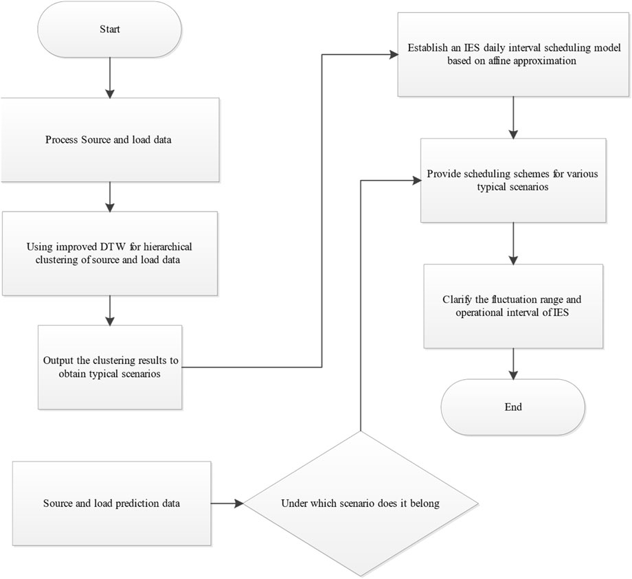
Figure 7. IES day-ahead scheduling based on improved DTW

5 Case study

To validate the rationality and accuracy of the method proposed in this paper, a specific regional PIEHS was selected as the research subject. The structure of this PIEHS is shown in Figure 1, where no related thermal product production activities are conducted during the night. One set each of wind and solar units, CHP units, and EB units is operational, with a 24-h operational cycle and a 15-min scheduling interval. In this paper, the selection of noise sources is described by Feixiong et al. (2023), the natural gas price is taken as 2.7, and the time-of-use electricity pricing mechanism is presented in Table 2. The parameters and settings of each piece of equipment are detailed by Zhang et al. (2023); Wei and Bai (2009); Rafique et al. (2018). The superiority and accuracy of the method proposed in this paper are verified through a comparison of scenarios. The computational hardware platform for the text is a PC with a 2.30 GHz Intel Core i5-6300HQ CPU and 8.00 GB of RAM.

Table 2

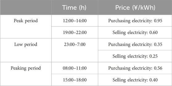
Table 2. Time-sharing electricity pricing mechanism.

5.1 Clustering result comparison

To evaluate the superiority of the clustering results, the SSE, DBI, and DVI were used as evaluation metrics. Two scenarios were used to compare and analyze the proposed method: Scheme 1 using DTW hierarchical clustering and Scheme 2 using hierarchical clustering of improved DTW. The hierarchical clustering center results under the two schemes are shown in Figure 8.

Figure 8

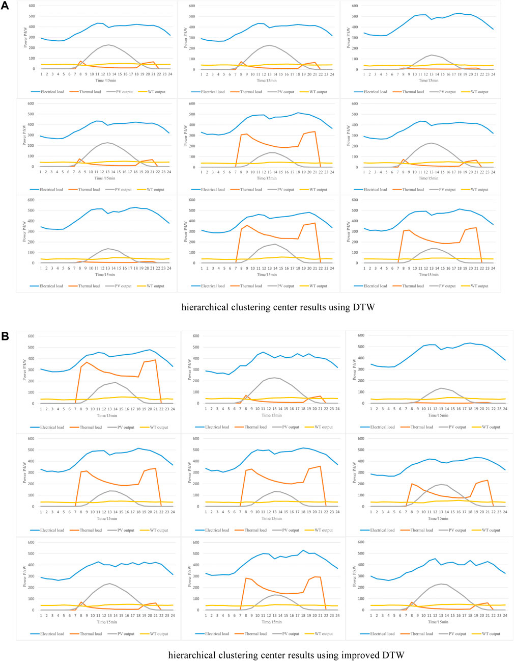
Figure 8. Hierarchical clustering center results.

As shown in Figure 8, after hierarchical clustering, there is no difference in the number of generated results between Schemes 1 and 2, both generating nine scenarios. Therefore, the two schemes were assessed using the SSE index, DBI index, and DVI index. The results for each index can be found in Table 3, while the computation time for both schemes is presented in Table 4.

Table 3

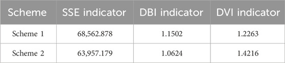
Table 3. Evaluation indicators under two schemes.

Table 4

Table 4. Computation time under two schemes.

From Table 3, it can be seen that the SSE index of Scheme 1 is larger than that of Scheme 2, indicating that the distance from the data in Scheme 1 to the cluster center is greater than that in Scheme 2. The DBI index of Scheme 1 is also larger than that of Scheme 2, indicating that the distance within the data cluster in Scheme 2 is smaller and closer to the cluster center. The DVI index of Scheme 2 is larger than that of Scheme 1, indicating that the distance between data clusters in Scheme 2 is larger and the distance within clusters is smaller. These three metrics show that the quality of clustering under Scheme 2 is better. As can be seen from Table 4, it is because of the better quality of clustering in Scheme 2 that the time used for iteration of Scheme 1 is greater than that of Scheme 2. Both the clustering metrics and the time taken show that the selection of clustering centers in Scheme 2 is better than that in Scheme 1, improving the accuracy of clustering.

In essence, the algorithm proposed in this article can guarantee convergence to a near-global optimum solution. This is because the algorithm is a greedy algorithm that minimizes the distance between data samples by continuously adjusting the time alignment between them. At each iteration, the algorithm selects the two closest data samples to merge until all data samples are merged. Such a greedy strategy essentially ensures that each step operates on the data pair with the smallest distance, allowing the algorithm to achieve a near-optimal solution.

5.2 Interval affine scheduling results

This article aims to provide interval affine scheduling schemes for all scenarios, focusing on scenario 1 (top left corner) as the scheduling object. As PIEHS is active only during 08:00–22:00 for related thermal product and production activities, a power system analysis is conducted to analyze the scheduling results. A comparative analysis of the two schemes is presented as follows:

Scheme 3 represents PIEHS interval scheduling, and Scheme 4 represents PIEHS interval affine scheduling. The power system interval dispatching of PIEHS is illustrated in Figure 9.

Figure 9

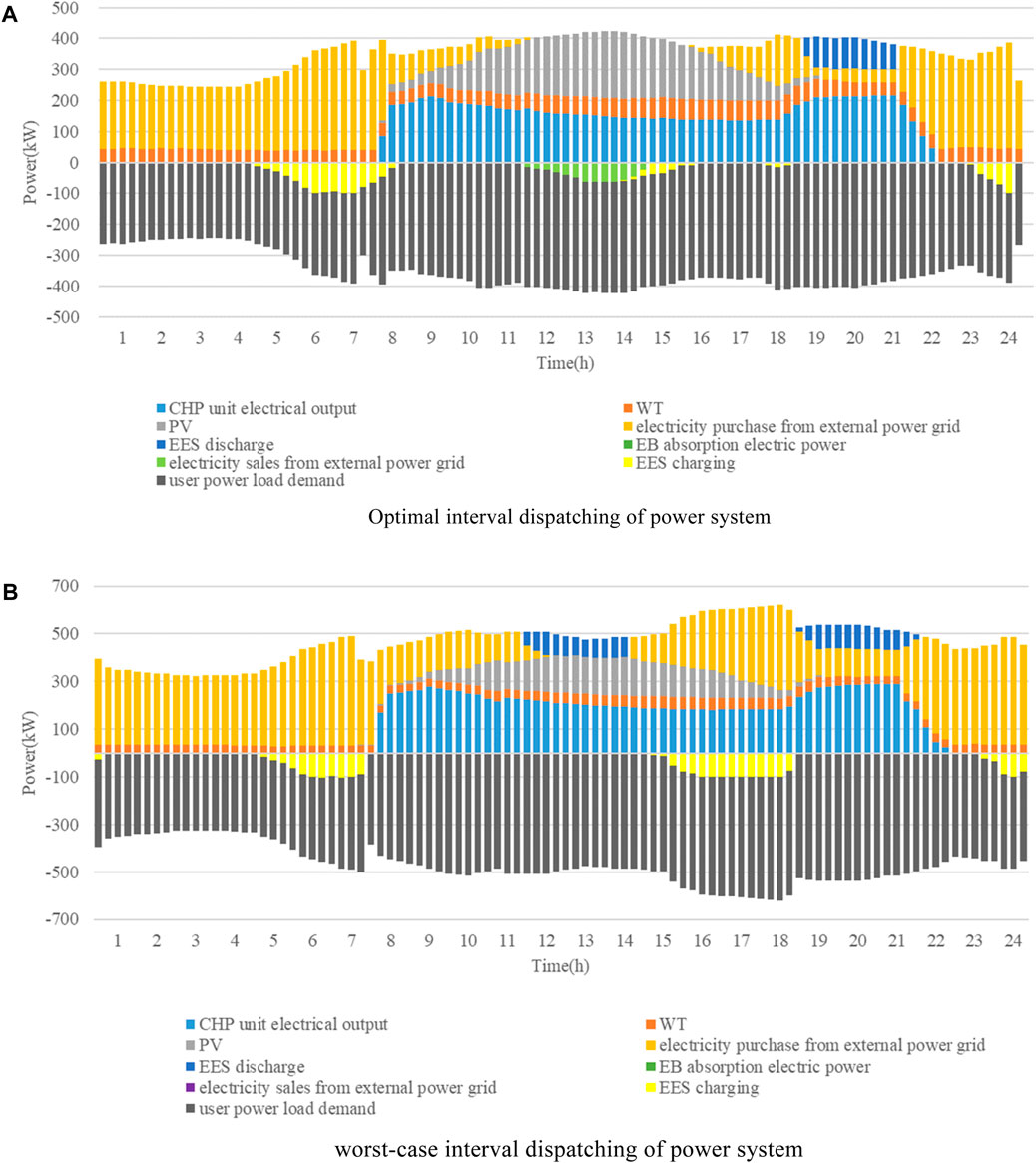
Figure 9. Interval dispatching in the PIEHS power system.

In PIEHS interval dispatching, the optimal operation condition is characterized by the minimum load demand and the highest new energy output, while the worst operation condition is characterized by the maximum load demand and the lowest new energy output. Transforming the uncertain scheduling problem into two deterministic problems, Table 5 lists the scheduling costs under interval operating conditions, ranging from 4,091.85 to 6,630.96. The output of various types of equipment in the power system is detailed in Table 6.

Table 5

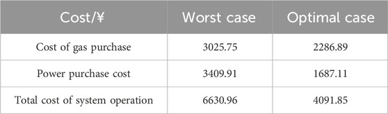
Table 5. PIEHS interval scheduling cost.

Table 6

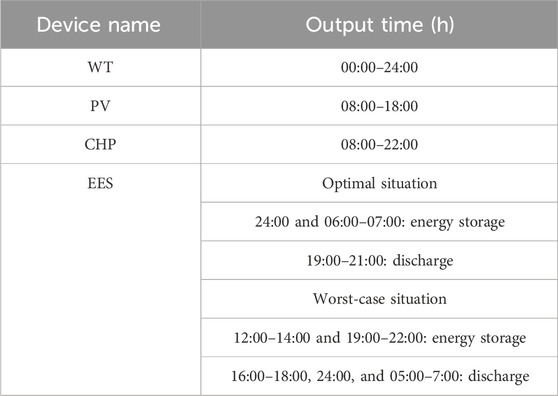
Table 6. PIEHS power system interval dispatch equipment output time.

As shown in Figure 9, the wind speed in this region is relatively stable, resulting in consistent wind power output throughout the day. The primary period of wind power output is from 08:00 to 18:00. The CHP unit operates in a “heat-based power” mode, with its output influenced by thermal load, operating only between 08:00 and 22:00. The EB unit does not contribute to the output. Under the optimal operation condition, only wind power is available between 23:00 and 07:00, failing to meet the electrical load demand. Therefore, electricity needs to be purchased from the higher-level power grid. The periods of 24:00 and 06:00–07:00 fall during the low electricity price period, allowing for the storage of excess energy. During 12:00–15:00, the source-end output meets the load requirement, eliminating the need to purchase electricity from the higher-level grid. In this period, it is also possible to sell excess electricity to the higher-level grid, resulting in a profit. The hours 19:00–21:00 represent the peak electricity price period, during which the CHP unit’s output reaches its maximum, with excess energy being discharged to compensate for the difference between the source and load, reducing the cost of purchasing electricity. Under the worst operation condition, the energy storage device discharges energy to the system during the peak periods of 12:00–14:00 and 19:00–22:00. Additionally, during the periods of 16:00–18:00, 24:00, and 05:00–07:00, excess energy is stored. In this scenario, the new energy output is low, the load demand is high, and there is no excess energy available for sale to the higher-level grid.

In contrast to interval scheduling, which transforms uncertain problems into two deterministic problems, this study constructs a PIEHS scheduling model based on affine transformations. Through affine arithmetic, the correlation between uncertain variables is represented by noise elements. The scheduling cost range calculated by interval affine is between 4,639.07 and 5,987.97, as shown in Table 7. After considering the correlation between uncertain variables, the scheduling range of Scheme 4 is smaller and less conservative than the scheduling cost range of Scheme 3.

Table 7

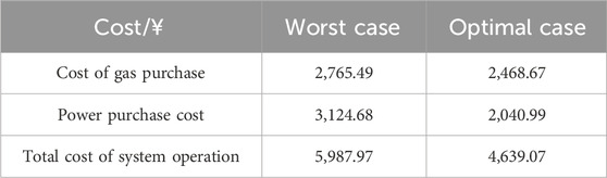
Table 7. PIEHS interval affine scheduling cost.

The output of various types of equipment in the power system under interval affine scheduling is shown in Table 8.

Table 8

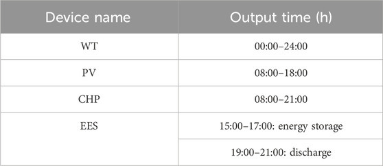
Table 8. PIEHS power system interval affine scheduling equipment output time.

Based on Figure 10, it can be observed that the PIEHS interval scheduling problem based on the affine algorithm is transformed into a deterministic scheduling problem centered around the interval and a fluctuation problem based on the interval radius. There is no need for dispatchers to choose between optimal or suboptimal scheduling solutions. At this point, the predictive data are transformed into cluster center data, and the fluctuation range of uncertain variables is also better provided for dispatchers’ reference. In Scheme 4, the EB is not operated due to the influence of operational costs and thermal loads. During the time periods of 11:00 and 14:00–18:00, the system is susceptible to fluctuations in electrical load. During the time period of 23:00–07:00, the electricity price is low, and the electrical load requirement is met by purchasing electricity from external sources. During this time, the fluctuation of the power system is mainly resolved by purchasing electricity from the higher-level power grid. The energy storage device is charged during the time periods of 15:00–17:00 and discharged during the time periods of 12:00–14:00. The energy storage device charges when the electricity price is low and discharges when the electricity price is high, reducing the operational cost of the system. During the time period of 08:00–21:00, the power system is susceptible to changes in thermal load and variations in the output of new energy sources. Since the CHP unit operates in the “heat-based power” mode, its output is limited by the coupling relationship between electricity and heat. The impact of uncertainty on the power system can be mitigated by discharging from the energy storage device and purchasing electricity from external sources. Among these, the CHP unit has the lowest output and the highest electricity price during the time period of 12:00–14:00; therefore, the discharge from the energy storage device is selected during this time. The comparison between Schemes 3 and 4 is shown in Tables 9 and 10.

Figure 10

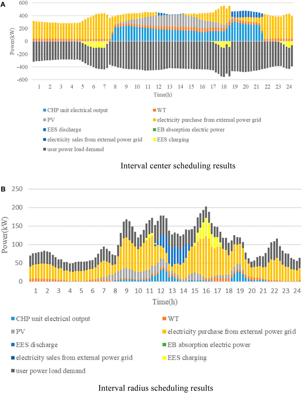
Figure 10. Interval affine scheduling for the PIEHS power system.

Table 9

Table 9. Cost comparison under optimal conditions.

Table 10

Table 10. Cost comparison under worst conditions.

Compared to interval scheduling, interval affine scheduling can take into account the correlation between various uncertainties, allowing for the rational utilization of CHP units, energy storage devices, and the higher-level power grid to reduce fluctuations. This achieves a better level of conservatism than Scheme 3. The results obtained also provide a more accurate reference for dispatchers.

6 Conclusion

The PIEHS interval affine scheduling proposed in this paper, based on the improved dynamic time warping algorithm, addresses current issues in PIEHS day-ahead scheduling. The main conclusions are as follows:

1) The hierarchical clustering method using the enhanced dynamic time warping algorithm avoids issues of length inconsistency caused by missing data in an interval time series. By analyzing the clustering results using the SSE metric, the SSE index for the improved hierarchical clustering is 63,957.179, a reduction of 4,605.699 compared to the pre-improvement value of 68,562.878. This indicates that the method proposed in this paper can perform accurate clustering for interval time-series data.

2) The scheduling cost range based on the interval algorithm is 4,091.85–6,630.96, while that based on the affine algorithm is 4,639.07–5,987.97. From this, it can be observed that the day-ahead interval scheduling model based on the affine algorithm can improve the conservatism of the interval scheduling results and consider the correlation of various uncertain variables. Moreover, based on the affine radius, the fluctuation range of each uncertain variable can be clearly determined, resulting in results that are more useful for reference by scheduling personnel.

Subsequent research efforts can delve deeper from the perspectives of considering load response characteristics and multi-energy coupling.

Data availability statement

The original contributions presented in the study are included in the article/Supplementary material; further inquiries can be directed to the corresponding author.

Author contributions

BL: writing–original draft.

Funding

The author(s) declare that no financial support was received for the research, authorship, and/or publication of this article.

Conflict of interest

The author declares that the research was conducted in the absence of any commercial or financial relationships that could be construed as a potential conflict of interest.

Publisher’s note

All claims expressed in this article are solely those of the authors and do not necessarily represent those of their affiliated organizations, or those of the publisher, the editors, and the reviewers. Any product that may be evaluated in this article, or claim that may be made by its manufacturer, is not guaranteed or endorsed by the publisher.

References

Ahmad, A., Khizar, S., Ghulam, H., Sadia, M., Sheraz, K., and Farrukh, A. K. (2023). Real-time energy optimization and scheduling of buildings integrated with renewable microgrid. Appl. Energy, 335. doi:10.1016/j.apenergy.2023.120640

CrossRef Full Text | Google Scholar

Antonazzi, E., Di Lorenzo, G., Stracqualursi, E., and Araneo, R. (2023). Renewable energy communities for sustainability: a case study in the metropolitan area of Rome. IEEE Ind. Comm. Power Syst. Eur., 1–6. doi:10.1109/EEEIC/ICPSEurope57605.2023.10194850

CrossRef Full Text | Google Scholar

Bai, L., Li, F., Cui, H., Jiang, T., Sun, H., and Zhu, J. (2016). Interval optimization based operating strategy for gas-electricity integrated energy systems considering demand response and wind uncertainty. Appl. Energy 167, 270–279. doi:10.1016/j.apenergy.2015.10.119

CrossRef Full Text | Google Scholar

Duan, P., Zhao, B., Zhang, X., and Fen, M. (2023). A day-ahead optimal operation strategy for integrated energy systems in multi-public buildings based on cooperative game. Energy 275, 127395. doi:10.1016/j.energy.2023.127395

CrossRef Full Text | Google Scholar

Ezugwu, A. E., Ikotun, A. M., Oyelade, O. O., Abualigah, L., Agushaka, J. O., Eke, C. I., et al. (2022). A comprehensive survey of clustering algorithms: state-of-the-art machine learning applications, taxonomy, challenges, and future research prospects. Eng. Appl. Artif. Intell. 110, 104743. doi:10.1016/j.engappai.2022.104743

CrossRef Full Text | Google Scholar

Feixiong, C., Mingjie, C., Yimin, L., Yixin, G., and Zhenguo, S. (2023). Affine optimization method for electrical-thermal interconnected systems considering multiple uncertainties. Proc. CSEE, 7467–7483. doi:10.13334/j.0258-8013.pcsee.220501

CrossRef Full Text | Google Scholar

Ghulam, H., Khurram, S. A., Zahid, W., Imran, K., Muhammad, U., Abdul, B. Q., et al. (2020). An innovative optimization strategy for efficient energy management with day-ahead demand response signal and energy consumption forecasting in smart grid using artificial neural network. IEEE Access 8, 84415–84433. doi:10.1109/ACCESS.2020.2989316

CrossRef Full Text | Google Scholar

Gong, D., Xu, B., Zhang, Y., Guo, Y., and Yang, S. (2020). A similarity-based cooperative co-evolutionary algorithm for dynamic interval multiobjective optimization problems. IEEE Trans. Evol. Comput. 24, 142–156. doi:10.1109/TEVC.2019.2912204

CrossRef Full Text | Google Scholar

Gunawan, J., and Huang, C.-Y. (2021). An extensible framework for short-term holiday load forecasting combining dynamic time warping and LSTM network. IEEE Access 9, 106885–106894. doi:10.1109/ACCESS.2021.3099981

CrossRef Full Text | Google Scholar

Hafeez, G., Wadud, Z., Khan, I. U., Khan, I., Shafiq, Z., Usman, M., et al. (2020). Efficient energy management of IoT-enabled smart homes under price-based demand response program in smart grid. Sensors 20, 3155. doi:10.3390/s20113155

PubMed Abstract | CrossRef Full Text | Google Scholar

Hengyu, H., Minglei, B., Yi, D., Jinyue, Y., and Yonghua, S. (2023). Probabilistic integrated flexible regions of multi-energy industrial parks: conceptualization andcharacterization. Appl. Energy, 349. doi:10.1016/j.apenergy.2023.121521

CrossRef Full Text | Google Scholar

Holder, C., Middlehurst, M., and Bagnall, A. (2023). A review and evaluation of elastic distance functions for time series clustering. Knowl. Inf. Syst. 66, 765–809. doi:10.1007/s10115-023-01952-0

CrossRef Full Text | Google Scholar

Jena, C., Guerrero, J. M., Abusorrah, A., Al-Turki, Y., and Khan, B. (2022). Multi-objective generation scheduling of hydrothermal system incorporating energy storage with demand side management considering renewable energy uncertainties. IEEE Access 10, 52343–52357. doi:10.1109/ACCESS.2022.3172500

CrossRef Full Text | Google Scholar

Kalim, U., Ghulam, H., Imran, K., Sadaqat, J., and Nadeem, J. (2021). A multi-objective energy optimization in smart grid with high penetration of renewable energy sources. Appl. Energy, 299. doi:10.1016/j.apenergy.2021.117104

CrossRef Full Text | Google Scholar

Kan, R., Hongliang, Y., Guohua, G., and Qian, C. (2019). Pulses classification based on sparse auto-encoders neural networks. IEEE Access 7, 92651–92660. doi:10.1109/ACCESS.2019.2927724

CrossRef Full Text | Google Scholar

Laszlo, T. (2010). Monte Carlo method for identification of outlier molecules in QSAR studies. J. Math. Chem. 47, 174–190. doi:10.1007/s10910-009-9540-6

CrossRef Full Text | Google Scholar

Li, Y., Han, M., Shahidehpour, M., Li, J., and Long, C. (2023). Data-driven distributionally robust scheduling of community integrated energy systems with uncertain renewable generations considering integrated demand response. Appl. Energy 335, 120749. doi:10.1016/j.apenergy.2023.120749

CrossRef Full Text | Google Scholar

Liu, H., and Chen, C. (2019). Data processing strategies in wind energy forecasting models and applications: a comprehensive review. Appl. Energy 249, 392–408. doi:10.1016/j.apenergy.2019.04.188

CrossRef Full Text | Google Scholar

Liu, J., Li, Y., Ma, Y., Qin, R., Meng, X., and Wu, J. (2023). Two-layer multiple scenario optimization framework for integrated energy system based on optimal energy contribution ratio strategy. Energy 285, 128673. doi:10.1016/j.energy.2023.128673

CrossRef Full Text | Google Scholar

Ma, Z., Yang, M., Jia, W., and Ding, T. (2022). Decentralized robust optimal dispatch of user-level integrated electricity-gas-heat systems considering two-level integrated demand response. Front. Energy Res. 10, 10. doi:10.3389/fenrg.2022.1030496

CrossRef Full Text | Google Scholar

Martínez Ceseña, E. A., Loukarakis, E., Good, N., and Mancarella, P. (2020). Integrated electricity-heat–gas systems: techno–economic modeling, optimization, and application to multienergy districts. Proc. IEEE 108, 1392–1410. doi:10.1109/JPROC.2020.2989382

CrossRef Full Text | Google Scholar

Rafique, M. K., Haider, Z. M., Mehmood, K. K., Zaman, M. S. U., Irfan, M., Khan, S. U., et al. (2018). Optimal scheduling of hybrid energy resources for a smart home. Energies 11, 3201. doi:10.3390/en11113201

CrossRef Full Text | Google Scholar

Ran, X., Zhang, J., Zhu, W., Liu, K., and Liu, Y. (2024). A model of correlated interval–probabilistic conditional value-at-risk and optimal dispatch with spatial correlation of multiple wind power generations. Int. J. Electr. Power Energy Syst. 155, 109500. doi:10.1016/j.ijepes.2023.109500

CrossRef Full Text | Google Scholar

Sajjad, A., Kalim, U., Ghulam, H., Imran, K., Fahad, R. A., and Syed, I. H. (2022). Solving day-ahead scheduling problem with multi-objective energy optimization for demand side management in smart grid. Eng. Sci. Technol., 36. doi:10.1016/j.jestch.2022.101135

CrossRef Full Text | Google Scholar

Santiago, R., Bergamaschi, F., Bustince, H., Dimuro, G., Asmus, T., and Sanz, J. A. (2020). On the normalization of interval data. Mathematics 8, 2092. doi:10.3390/math8112092

CrossRef Full Text | Google Scholar

Shang, C., Gao, J., Liu, H., and Liu, F. (2021). Short-term load forecasting based on PSO-KFCM daily load curve clustering and CNN-LSTM model. IEEE Access 9, 50344–50357. doi:10.1109/ACCESS.2021.3067043

CrossRef Full Text | Google Scholar

Shuai, C., Sun, Y., Zhang, X., Yang, F., Ouyang, X., and Chen, Z. (2023). Intelligent diagnosis of abnormal charging for electric bicycles based on improved dynamic time warping. IEEE Trans. Ind. Electron 70, 7280–7289. doi:10.1109/TIE.2022.3206702

CrossRef Full Text | Google Scholar

Tran, L., and Duckstein, L. (2002). Comparison of fuzzy numbers using a fuzzy distance measure. Fuzzy Sets Syst. 130, 331–341. doi:10.1016/S0165-0114(01)00195-6

CrossRef Full Text | Google Scholar

Wei, H., and Bai, X. (2009). Semi-definite programming-based method for security-constrained unit commitment with operational and optimal power flow constraints. IET Gener. Transm. Distrib. 3 (2), 182–197. doi:10.1049/iet-gtd:20070516

CrossRef Full Text | Google Scholar

Xiong, H., Chen, Z., Zhang, X., Wang, C., Shi, Y., and Guo, C. (2023). Robust scheduling with temporal decomposition of integrated electrical-heating system based on dynamic programming formulation. IEEE Trans. Ind. Appl. 59, 1–13. doi:10.1109/TIA.2023.3263385

CrossRef Full Text | Google Scholar

Xu, J., Wang, X., Gu, Y., and Ma, S. (2023). A data-based day-ahead scheduling optimization approach for regional integrated energy systems with varying operating conditions. Energy 283, 128534. doi:10.1016/j.energy.2023.128534

CrossRef Full Text | Google Scholar

Yang, X., Wang, X., Deng, Y., Mei, L., Deng, F., and Zhang, Z. (2023). Integrated energy system scheduling model based on non-complete interval multi-objective fuzzy optimization. Renew. Energy 218, 119289. doi:10.1016/j.renene.2023.119289

CrossRef Full Text | Google Scholar

Yansong, W., Shuangyu, L., Renjie, M., Chengbo, N., and Jingbo, Y. (2023). Optimization planning of oil field comprehensive energy system based on interval theory. Electr. Power Autom. Equip., 1–15. doi:10.16081/j.epae.202305010

CrossRef Full Text | Google Scholar

Zhang, M., Yu, S., and Li, H. (2023). Inter-zone optimal scheduling of rural wind–biomass-hydrogen integrated energy system. Energies 16, 6202. doi:10.3390/en16176202

CrossRef Full Text | Google Scholar

Zheng, W., Wang, X., Shao, Z., Zhang, M., and Li, Y. (2022). A modified affine arithmetic-based interval optimization for integrated energy system with multiple uncertainties. J. Renew. Sustain. Energy 14, 016302. doi:10.1063/5.0079306

CrossRef Full Text | Google Scholar

Nomenclature