Electricity consumption optimization of power users driven by a dynamic electric carbon factor

1 Introduction

Global fossil energy-related emissions include carbon dioxide emitted from the combustion of coal, oil and gas, and cement production (Zhang et al., 2023). Recent analyses by the International Energy Agency (IEA) suggest that global fossil energy-related emissions could peak in 2023 as the growth of clean energy sources accelerates and the use of fossil fuels declines. However, failed projections in the past could undermine hopes that global emissions are about to peak. As early as 2016, there were indications that global emissions had peaked and would decline. Similarly, in the wake of the novel coronavirus outbreak, many researchers estimated that global fossil energy-related emissions peaked in 2019 (Zhang et al., 2020; Zeng et al., 2023a).

Fossil energy-related emissions hit new records in both 2022 and 2023. Just as importantly, reducing the growth in annual emissions will not stop carbon dioxide from accumulating in the atmosphere or prevent the world from continuing to warm. In order to help reduce carbon emissions down to net zero, this study selects typical energy-intensive users, simulates their carbon emission behavior under the control of a dynamic electro-carbon factor, and provides them with a low-carbon electricity consumption optimization scheme (Ruhnau et al., 2022; Sun and Huang, 2022; Yan et al., 2023).

The selection of which businesses to analyze as typical requires consideration of a number of factors, including the size of the business, type of industry, geographic location, energy consumption patterns, and so on. The following are some of the types of enterprises that may be suitable for analysis as a typical enterprise: first, energy-intensive enterprises: these enterprises, such as large-scale industrial enterprises, usually consume large amounts of energy and involve complex production processes and equipment, e.g., steel mills, chemical plants, and automobile manufacturing plants. Second, commercial and service enterprises: these enterprises, such as supermarkets, shopping malls, and hotels, may have unique patterns of energy consumption, such as large amounts of lighting, air-conditioning, and refrigeration equipment. In this paper, in order to significantly reduce carbon emissions and energy loss, high-energy-consuming enterprises are selected as the research object.

Regarding electricity user behavior, Papachristos (2015) developed a distributed microgeneration model considering whether living on a property with on-site renewable generation affects user attitudes and behavior. Stedmon et al. (2013) conducted research on user behavior in relation to electricity consumption in office buildings and residential environments. Martinez-Gil et al. (2013) mapped the user behavioral profiles based on household electricity demand at specific times of the day and analyzed specific-purpose electricity use activities, time-of-use surveys, and smart meter data for a family of four. Laicane et al. (2015) further analyzed household electricity use by testing the extent to which building factors, socio-demographics, and appliance ownership explain the annual electricity consumption in residential buildings using gas for space and hot water heating. Huebner et al. (2016) encouraged sustainable consumer behavior change in electricity use through the social dimension. For a bottom-up modeling approach, White et al. (2019) demonstrated the impact of electricity usage patterns on electricity consumption by analyzing the interactions between household user efficiency, smart meter penetration, and consumer behavior.

In a recent study on international carbon emissions, Saint Akadiri et al. (2020) examined the link between carbon emissions, electricity consumption, economic growth, and globalization in Turkey. Abbasi et al. (2021) mined the dynamic causal relationship between energy consumption, carbon emissions, and economic growth in Pakistan. Lin and Jia(2020) analyzed the drivers of carbon emissions from electricity in EU countries based on the LMDI-I approach. Abbasi and Adedoyin (2021) compared the carbon emissions generated by the coal heating method and the electric heating method in northern China and found that energy substitution is not energy efficient and, therefore, needs to be combined with other energy-saving policies.

Currently, carbon emissions are calculated in the following ways: emission factor method: carbon emissions are calculated using a pre-determined carbon emission factor based on the type and use of energy (Grygar and Fabricius, 2019). This method is simple and intuitive, and it is often used to estimate carbon emissions from energy consumption. Process analysis method: by analyzing the energy consumption and emissions of each link in the production process in detail, the carbon emissions of each link are calculated and then aggregated to arrive at the overall emissions. This method is suitable for in-depth analysis and optimization of production processes. Input–output analysis: it is also known as life cycle assessment (LCA); this method takes into account the entire life cycle of a product or service, including the stages of raw material acquisition, production, use, and disposal, and calculates carbon emissions over the entire life cycle. Methods based on energy statistics: carbon emissions are estimated using energy statistics and energy consumption, combined with parameters such as energy emission factors. This method is often used to assess the carbon emissions of large-scale or large-scale energy systems. Model simulation method: based on physical or mathematical models, the operation of the energy system is simulated, including energy conversion, energy consumption, and emission processes, in order to calculate carbon emissions (Suzuki et al., 2020). Each of these calculation methods has its own advantages and disadvantages, and the main shortcomings include the following: 1). uncertainty of data: the data required for calculating carbon emissions usually come from multiple sources, and there are uncertainties and errors that affect the accuracy and reliability of the results. 2). Scope limitations: different calculation methods are limited in their scope of application. For example, the emission factor method is suitable for estimating carbon emissions from energy consumption, but it cannot take into account all emissions during the life cycle. 3). Complexity and time consumption: some calculation methods (e.g., process analysis and life cycle assessment) require detailed analysis of the entire life cycle of a production process or product, which requires a large amount of data and takes a long time.

Furthermore, multi-objective optimization (Hancer et al., 2018) is an optimization method that involves multiple objective functions in a decision problem. There are usually conflicting or non-comparable objectives in a multi-objective problem, so it is not possible to simply find a solution that maximizes or minimizes all the objectives at the same time. The aim of multi-objective optimization is to find a set of solutions that form a non-dominated set, called a “Pareto frontier,” which outperforms other solutions on all objectives (Boyaci et al., 2022; Liu et al., 2022; Zeng et al., 2023b; Liu et al., 2023).

Drawing inspiration from these sources, this paper delves into the diverse modes of production behavior by examining the electricity consumption patterns of energy-intensive enterprises. It introduces a novel approach for optimizing electricity usage based on dynamic electro-carbon factors. Guided by these factors, the proposed technique offers robust support for users aiming to conserve energy and minimize emissions (Xiao et al., 2023a). The study scrutinizes the electricity consumption behavior across four distinct types of energy-intensive factories, considering variations in their production modes throughout the year. Notably, it accounts for both regular electricity consumption costs and peak usage expenses. Furthermore, the analysis extends to evaluating the comfort level associated with electricity usage. Focused on electricity cost, carbon emissions, and electricity usage comfort, this research endeavors to aid energy-intensive companies in curbing their expenditure and environmental impact while maintaining high productivity (Xiao et al., 2023b).

The subsequent sections are structured as follows: Section 2 outlines the mathematical model of automatic response modeling for high-energy demand (ARM-HED). Section 3 provides the simulation validation for ARM-HED. Section 4 presents the simulation findings and discussions pertaining to the four distinct production models. Finally, Section 5 offers concluding remarks.

2 Automatic response modeling for high-energy demand

This study focuses on industrial parks predominantly housing energy-intensive industries as its primary research subjects. It meticulously analyzes various operational data from these industries and formulates an automatic response model tailored to their energy-demand characteristics.

The automatic response modeling for high energy demand represents a sophisticated mathematical framework. This model scrutinizes the ramifications of electricity consumption by high-energy-consuming industries on the power grid. It integrates a dynamic electro-carbon factor to drive reductions in carbon emissions while assessing electricity cost, carbon emissions, and user comfort as key evaluation criteria. The overarching goal is to devise scenarios that optimize resource utilization, minimize carbon footprints, and uphold user comfort. ARM-HED holds significant applicability in the energy planning, policymaking, and investment decision-making arenas. It serves as a valuable tool in realizing carbon reduction objectives, enhancing the sustainability of energy systems, and reducing energy expenses. In doing so, it contributes meaningfully to sustainable development endeavors and the global fight against climate change.

This paper delves into the behavioral dynamics of electricity consumption within energy-intensive industries, employing the dynamic electro-carbon factor as a catalyst to categorize operational electricity demands into four distinct scenarios.

In defining the index for reducing carbon emissions from energy-consuming industries, the carbon emitted by these industries due to electricity consumption is quantified using the following Eq. 1:

${\delta }_{\mathrm{s}}=\frac{P_{\mathrm{g}}\times {\delta }_{\mathrm{g}}+{\displaystyle {\sum }_{j\in {\mathrm{\Omega }}_s}}{P}_{so}\times {\delta }_n}{P_{\mathrm{g}}+{\displaystyle {\sum }_{o\in {\mathrm{\Omega }}_s}}{P}_{so}}.(1)$

In the above equation, ${\delta }_s$ denotes the electro-carbon index of the sth high-energy-consuming enterprise; $P_{\mathrm{g}}$ denotes the active power output from the generation port connected to the gth enterprise; ${\delta }_{\mathrm{g}}$ is the electro-carbon index of the connected generation port; $P_{so}$ is the branch active power that flows from the sth node to the oth node; ${\mathrm{\Omega }}_s$ denotes the set of nodes connected to the sth high-energy-consuming enterprise’s branches; and ${\delta }_o$ is the oth node’s electro-carbon index.

In certain scenarios, it may be viable to disregard the impact of the grid power command response factor, which is contingent upon whether the energy-intensive enterprise has established an agreement with the local grid company. Should such an agreement not exist, the enterprise retains the autonomy to adjust its power consumption plan spontaneously, factoring in variables such as electricity prices and energy consumption costs. Within the power system framework, enhancing consumer flexibility and responsiveness carries positive implications for grid stability and reliability.

Among energy-intensive enterprises, certain industrial users possess greater load flexibility, enabling them to swiftly adjust their loads in response to grid commands, potentially resulting in fluctuations in overall electricity consumption. Conversely, other enterprises exhibit a more static demand for electricity, leading to negligible changes in overall consumption even in response to grid commands. As such, the four scenarios of electricity consumption behavior are delineated as follows.

• Plant type 1: the enterprise does not have an agreement with the local grid company, and the enterprise has a fixed demand for electricity; the overall electricity consumption does not change before or after the response. The demand response optimization model for this case can be described as Eq. 2:

$\left\{\begin{array}{c}\min F={\displaystyle {\sum }_{t=1}^T}\left(\overline{P_{\mathrm{L}}}\left(t\right)\times {\lambda }_{\mathrm{E}}\left(t\right)\right)+{\displaystyle {\sum }_{t=1}^T}{\displaystyle {\sum }_{\mathrm{s}}^{\mathrm{o}}}\left(\overline{P_{\mathrm{L}}}\left(t\right)\times {\delta }_{\mathrm{s}}\times {\lambda }_{\mathrm{C}}\left(t\right)\right)\\ st.{\displaystyle {\sum }_{t=1}^T}\overline{P_{\mathrm{L}}}\left(t\right)={\displaystyle {\sum }_{t=1}^T}{P}_{\mathrm{L}}\left(t\right)\\ \left(1-\delta \left(t\right)\right)\bullet P_{\mathrm{L}}\left(t\right)\le \overline{P_{\mathrm{L}}}\left(t\right)\le P_{\mathrm{L}}^{\max },t=1,2,\cdots ,T\end{array}\right.,(2)$

where F is the objective function of the model, $\overline{P_L}\left(t\right)$ is the corresponding enterprise’s power consumption in time period t, ${\delta }_{\mathrm{s}}$ denotes the electric carbon coefficient of the sth high-energy-consuming enterprise, o is the total number of enterprises, and ${\lambda }_{\mathrm{C}}\left(t\right)$ denotes the carbon tax required to be paid by the corresponding carbon emission in time period t. $P_L\left(t\right)$ is the original power consumption of the load of this industrial park in time period t; ${\lambda }_{\mathrm{E}}\left(t\right)$ is the electricity consumption price in time period t. $\delta \left(t\right)$ is the maximum reduction ratio of the loads in the park in time period t; $P_{\mathrm{L}}^{\max }$ indicates the maximum power consumption of the loads in the industrial park; and T is the number of time periods of power consumption.

To obtain the response for case 1, first, the electricity price curve of the grid where the industrial park is located, the peak and the valley periods of electricity consumption, the daily electricity consumption curve of the loads in the industrial park (24 h, one point per hour), the maximum curtailment ratio of each time period, and the maximum power consumption of the loads in the industrial park should be obtained.

• Plant type 2: the enterprise does not have an agreement with the local grid company, but the enterprise does not have a fixed demand for electricity. The tariff structure is based on a differentiated or peak and valley tariff system, and the enterprise has an incentive to adjust its electricity consumption behavior during peak hours; the overall electricity consumption may change with the response. This demand response optimization model can be described by the following Eq. 3:

$\left\{\begin{array}{c}\min F={\displaystyle {\sum }_{t=1}^T}\left(\overline{P_{\mathrm{L}}}\left(t\right)\times {\lambda }_{\mathrm{E}}\left(t\right)\right)+{\displaystyle {\sum }_{t=1}^T}{\displaystyle {\sum }_{\mathrm{s}}^{\mathrm{o}}}\left(\overline{P_{\mathrm{L}}}\left(t\right)\times {\delta }_{\mathrm{s}}\times {\lambda }_{\mathrm{C}}\left(t\right)\right)\\ st.{\displaystyle {\sum }_{t=1}^T}\overline{P_{\mathrm{L}}}\left(t\right)={\displaystyle {\sum }_{t=1}^T}{P}_{\mathrm{L}}\left(t\right)\\ \left(1-\delta \left(t\right)\right)\bullet P_{\mathrm{L}}\left(t\right)\le \overline{P_{\mathrm{L}}}\left(t\right)\le P_{\mathrm{L}}^{\max },t=1,2,\cdots ,T\end{array}\right.,(3)$

where $F_{\mathrm{E}}\left(t\right)$ is the price penalty coefficient corresponding to an enterprise’s electricity consumption load during the curtailment period; the greater the electricity consumption of the consumption end in an industrial park containing high-energy-consuming enterprises during a certain time period, the greater the penalty coefficient for the corresponding time period. $\beta$ is the cumulative maximum curtailment ratio of electricity consumption in an industrial park containing high-energy-consuming enterprises.

The response for plant type 2 requires the same inputs as those required for plant type 1 in terms of the local electricity price curve, peak and valley periods, load-normal electricity consumption curve, the maximum reduction ratio for each time period, and the maximum power consumption of the industrial park, in addition to the price penalty factor for the reduction of electricity consumption in the location of industrial parks containing high-energy-consuming enterprises, as well as the maximum reduction ratio of electricity consumption.

• Plant type 3: the enterprise has an agreement with the local grid company that it needs to respond to grid power orders. However, the energy-intensive enterprise has a fixed power demand, and the overall power consumption does not change before or after the response. The demand response optimization model for this case can be described as Eq. 4:

$\left\{\begin{array}{c}\min F={\displaystyle \sum _{t=1}^T}\left(\overline{P_{\mathrm{L}}}\left(t\right)\times {\lambda }_{\mathrm{E}}\left(t\right)\right)+{\displaystyle \sum _{t=1}^T}\left(P_L\left(t\right)-\overline{P_L}\left(t\right)\times F_{\mathrm{E}}\left(t\right)\right)+{\displaystyle \sum _{t=1}^T}{\displaystyle \sum _{\mathrm{s}}^{\mathrm{o}}}\left(\overline{P_{\mathrm{L}}}\left(t\right)\times {\delta }_{\mathrm{s}}\times {\lambda }_{\mathrm{C}}\left(t\right)\right)\\ st.{\displaystyle \sum _{t=1}^T}\overline{P_{\mathrm{L}}}\left(t\right)\ge \left(1-\beta \right)\bullet {\displaystyle \sum _{t=1}^T}{P}_{\mathrm{L}}\left(t\right)\\ \left(1-\delta \left(t\right)\right)\bullet P_{\mathrm{L}}\left(t\right)\le \overline{P_{\mathrm{L}}}\left(t\right)\le P_{\mathrm{L}}^{\max },t=1,2,\cdots ,T\end{array}\right.,(4)$

where T_C is the set of specified response periods of the power grid being modeled, e.g., the set of peak power consumption periods, and $P_{\mathrm{c}}^{\text{grid}}$ denotes the power consumption command sent by the grid.

The response inputs for plant type 3 are the same as those required for plant type 1 in terms of local tariff curves, peak and valley time periods, load-normal electricity consumption curves, maximum curtailment ratios for each time period, and maximum power consumption in industrial parks containing high-energy-consuming firms, in addition to the power consumption commands of the grid corresponding to the industrial parks containing the high-energy-consuming firms and the set of commanded response time periods, unlike plant types 1 and 2.

• Plant type 4: enterprises sign an agreement with the local grid company and need to consider the grid power command response. At the same time, this high-energy-consuming enterprise does not have a fixed power demand, and the overall power consumption of the enterprise can change with the response. The demand response optimization model for this case can be described as Eq. 5:

$\left\{\begin{array}{c}\min F={\displaystyle {\sum }_{t=1}^T}\left(\overline{P_{\mathrm{L}}}\left(t\right)\times {\lambda }_{\mathrm{E}}\left(t\right)\right)+{\displaystyle {\sum }_{t=1}^T}\left(P_L\left(t\right)-\overline{P_L}\left(t\right)\times F_{\mathrm{E}}\left(t\right)\right)+{\displaystyle {\sum }_{t=1}^T}{\displaystyle {\sum }_{\mathrm{s}}^{\mathrm{o}}}\left(\overline{P_{\mathrm{L}}}\left(t\right)\times {\delta }_{\mathrm{s}}\times {\lambda }_{\mathrm{C}}\left(t\right)\right)\\ st.{\displaystyle {\sum }_{t=1}^T}\overline{P_{\mathrm{L}}}\left(t\right)\ge \left(1-\beta \right)\bullet {\displaystyle {\sum }_{t=1}^T}{P}_{\mathrm{L}}\left(t\right)\\ {\displaystyle {\sum }_{t\in T_{\mathrm{c}}}}\overline{P_{\mathrm{L}}}\left(t\right)=P_{\mathrm{c}}^{\text{grid}}\\ \left(1-\delta \left(t\right)\right)\bullet P_{\mathrm{L}}\left(t\right)\le \overline{P_{\mathrm{L}}}\left(t\right)\le P_{\mathrm{L}}^{\max },t=1,2,\cdots ,T\end{array}\right..(5)$

The response inputs for plant type 4 need to be the same as those required for plant type 2 in terms of the electricity price curve for the region, the peak and valley time periods for electricity consumption, the normal electricity consumption curve for the industrial park containing the high-energy-consuming enterprise, the maximum reduction ratio for each time period, the maximum power consumption for the industrial park containing the high-energy-consuming enterprise, the electricity consumption reduction price penalty coefficient for the region in which the industrial park containing the high-energy-consuming enterprise is located, and the maximum reduction ratio of the electricity consumption, in addition to the grid electricity consumption directive, and a set of directive response time periods corresponding to the industrial park containing the high-energy-consuming enterprise as are required for plant type 3.

3 Simulation verification for ARM-HED

3.1 Load setting

This paper takes the industrial park of energy-consuming enterprises as the main research object, and four kinds of energy-consuming enterprises with different production modes are modeled. These four types of high-energy-consuming enterprises are 24-h continuous production factories, ecological peak production factories, pure daytime production factories, and pure nighttime production factories. In order to better distinguish the production characteristics of the four types of energy-intensive plants, Table 1 shows the production characteristics of these plants. The data for this table are derived from mobile phones and summarized from data on their production characteristics and electricity consumption behavior (Huwei et al., 2023).

Table 1

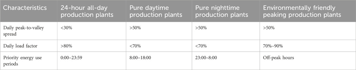
Table 1. Characteristics of four types of energy-intensive factory production.

The combination of a 24-hour all-day production plant, a pure daytime production plant, a pure nighttime production plant, and an environmentally friendly peaking production plant represents virtually all plant production modes.

The 24-hour all-day production plants: this enterprise operates 24 h a day. It is used for processes that require continuous production, such as certain chemical manufacturing or power generation facilities.

Pure daytime production plants: a daytime production plant operates only during daylight hours. This schedule is an option for industries where daylight is critical, such as construction or certain types of manufacturing.

Pure nighttime production plants: in contrast, nighttime production plants operate only at night. Industries with cooler temperatures or less traffic may prefer this type of production schedule, as it helps increase productivity.

Environmentally friendly peaking production plants: with an emphasis on environmental protection, this type of plant can use staggered production schedules to optimize energy use or reduce the environmental impact. Staggered production allows for a more even distribution of energy demand throughout the day, thereby reducing peak loads.

By combining these different production models, companies can tailor their operations to specific requirements, such as maximizing efficiency, minimizing energy consumption, or aligning with environmental sustainability goals. Each production model has its own advantages and considerations, and the choice depends on factors such as the nature of the industry, energy costs, and environmental priorities.

To provide a better presentation of the performance of the main research object, i.e., the four high-energy-consuming enterprises (represented by Model 1, Model 2, Model 3, and Model 4 in Figure 1) within the industrial park in a year, this paper solves the four high-energy-consuming enterprises as a model with four different production types (24-hour all-day production plants, pure daytime production plants, pure nighttime production plants, and environmentally friendly peaking production plants) and compares it with the interior point method (represented by FM) and the genetic algorithm (GA) for the solution. The schematic diagram is represented in Figures 2–5.

Figure 1

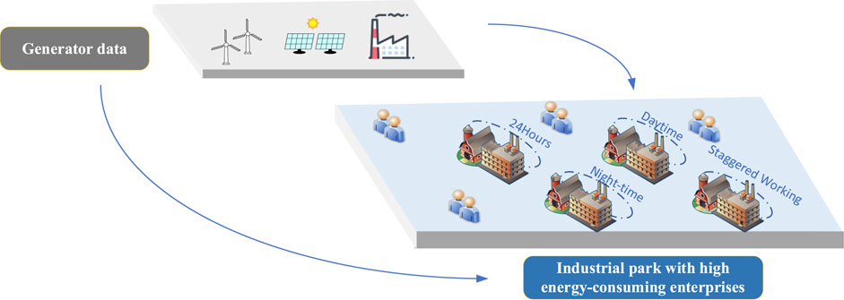
Figure 1. Schematic diagram of the framework of industrial parks and power plants for energy-consuming enterprises.

Figure 2

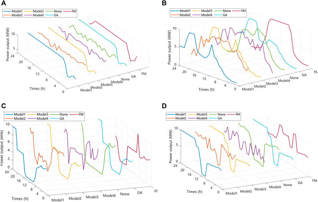
Figure 2. Comparison of power output of four different types of plants in the first quarter: (A) 24-hour all-day production plants, (B) Pure daytime production plants, (C) Pure nighttime production plants, (D) Environmentally friendly peaking production plants.

Figure 3

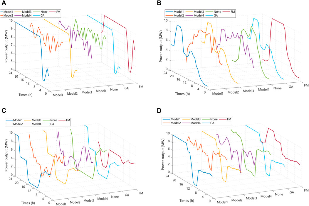
Figure 3. Comparison of power output of four different types of plants in the second quarter: (A) 24-hour all-day production plants, (B) Pure daytime production plants, (C) Pure nighttime production plants, (D) Environmentally friendly peaking production plants.

Figure 4

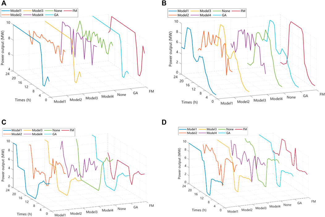
Figure 4. Comparison of power output of four different types of plants in the third quarter: (A) 24-hour all-day production plants, (B) Pure daytime production plants, (C) Pure nighttime production plants, (D) Environmentally friendly peaking production plants.

Figure 5

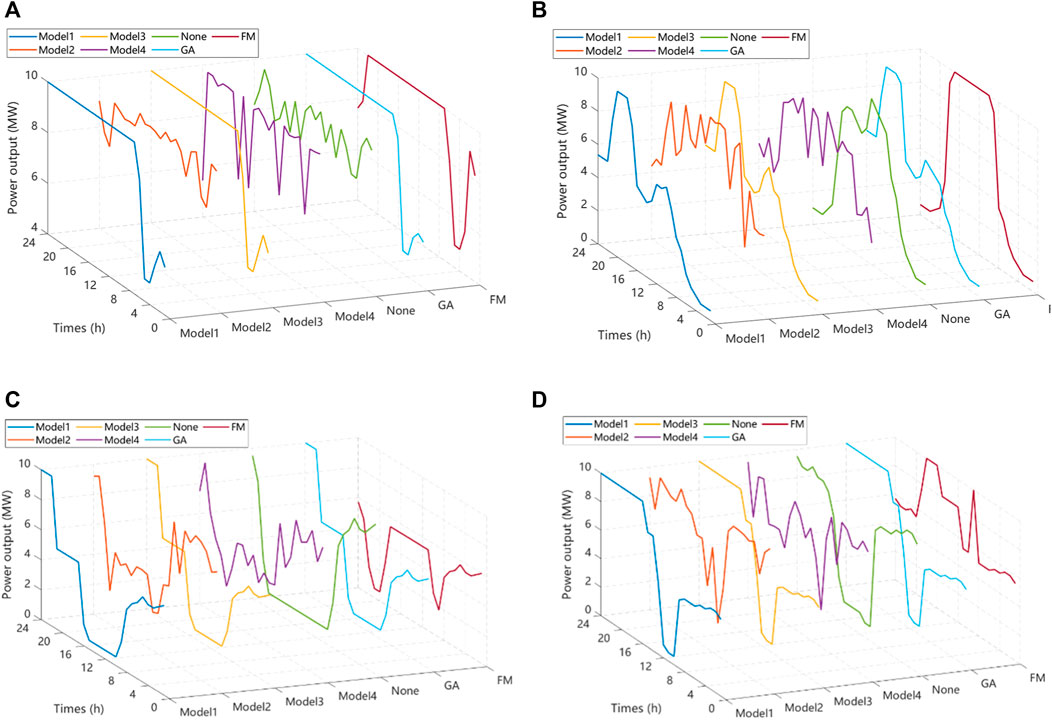
Figure 5. Comparison of power output of four different types of plants in the fourth quarter: (A) 24-hour all-day production plants, (B) Pure daytime production plants, (C) Pure nighttime production plants, (D) Environmentally friendly peaking production plants.

The interior point method is a numerical method for solving optimization problems and is particularly good for linear programming and convex optimization problems. As a single-objective algorithm, the interior point method is globally convergent, efficient, stable, and scalable. The interior point method can converge to the global optimal solution within a reasonable time without falling into the local optimal solution. Compared with other optimization algorithms, interior point methods usually have faster convergence and better computational efficiency. Specifically, its advantages are more obvious in high-dimensional problems and large-scale problems. Moreover, it usually shows good stability in the numerical solution process, is insensitive to the numerical characteristics of the problem, and has a wide range of applicability.

GA, as a single-objective optimization algorithm, has global search capability, parallelism and distribution, adaptability, solution space exploration capability, and robustness. The genetic algorithm is capable of conducting a global search, aiding in finding the global optimal solution by stochastically exploring the solution space, which is especially suitable for high-dimensional and nonlinear optimization problems. Genetic algorithms are naturally parallel and distributed, and they can process multiple solutions simultaneously and discover more potential solutions through crossover and mutation operations in the population, thus improving search efficiency. At the same time, it is able to adaptively adjust the search strategy and parameters dynamically according to the current progress in the search process, which is conducive to rapid convergence to the optimal solution. It is insensitive to the initial values and constraints of the problem, has good robustness, is applicable to various types of optimization problems, and requires fewer mathematical properties of the problem.

As can be seen from the graph, the fluctuation of 24-h continuous production plants is small, the fluctuation of pure daytime production plants is differentiated from pure nighttime production plants, and the characteristics of eco-peak production plants are closer to those of pure nighttime production plants. This suggests that these plants maintain a relatively stable production pattern without significant variations over time. The graph distinguishes between the fluctuation patterns of pure daytime and pure nighttime production plants. This differentiation implies that these two types of production plants exhibit distinct energy consumption or production behaviors, likely influenced by factors such as daylight availability and operational preferences. The characteristics of eco-peak production plants are noted to be closer to those of pure nighttime production plants. This implies that the eco-peak production plants, with a focus on peak production during specific periods, share similarities with the production behavior observed in pure nighttime plants.

3.2 Multi-targeting

Aiming at assisting energy-consuming enterprises to save energy and reduce emissions while, at the same time, considering the comfort of their electricity consumption and the cost associated with it, this paper introduces a dynamic electro-carbon factor as a driver, which takes the carbon emissions, the cost of electricity consumption, and the loss of electricity as the objectives to be considered at the same time.

In the case of energy-intensive companies, it is first necessary to analyze the structure and processes of their electricity consumption. By identifying and optimizing energy-inefficient equipment and systems, unnecessary energy waste can be reduced, and the overall efficiency of electricity consumption can be improved. Second, this paper introduces the dynamic electric-carbon factor to monitor carbon emissions in real time and provide a guarantee for energy savings and emission reduction. At the same time, the electricity cost structure is analyzed to identify the main electricity cost drivers. This helps develop targeted cost-reduction strategies, such as adopting alternative energy sources during peak hours and procuring more favorable power contracts. In addition, an electricity demand response program is developed to adjust the electricity consumption behavior of the company to the load profile of the grid. By reducing electricity demand during peak hours, electricity cost reduction and system stability improvement can be obtained. By taking into account energy efficiency, electricity costs, and employee comfort, companies can achieve sustainable energy savings and emissions reduction and improve the quality of the overall electricity environment while ensuring economic efficiency.

4 Case studies

4.1 Dataset and parameters of experiments

In the experiment, the above four load characteristic curves, four seasonal tariff variations, and four different energy-consuming enterprises’ electricity consumption optimization models are considered, and the electricity cost reduction, valley electricity consumption filling, and peak electricity consumption reduction before and after optimization are analyzed in different scenarios of different models. ${\lambda }_{\mathrm{E}}\left(t\right)$ is set as the corresponding seasonal tariff curve; $F_{\mathrm{E}}\left(t\right)$ adopts the principle that “the larger the customary period of electricity consumption, the larger the coefficient.” When the enterprise’s electricity consumption is greater than 70%, the coefficient is set to 10; when it is less than 30%, the coefficient is set to 1; and when it is located in the range of 30%–70%, the coefficient is set to 5; ${\lambda }_{\mathrm{L}}$ is set to 0.8. $T_{\mathrm{f}}$ is set according to the real-time grid tariff corresponding to the seasonal peak time of the grid, ${\lambda }_{\mathrm{E}}\left(t\right)>1$ is set to the time period ${t\in T}_{\mathrm{f}}$, and $F_{\mathrm{G}}$ is set to 4.

4.2 Statistical results

Taking the first quarter as an example, this experiment considers the carbon emission, electricity cost, and electricity comfort of four high-energy-consuming enterprises in the industrial park and obtains the following Pareto chart. A two-dimensional schematic of the multi-objective Pareto plane for the four high-energy-consuming firms in the first quarter is shown in Figure 6. A three-dimensional schematic of a multi-objective Pareto surface for a plant with 24-h continuous production for one season, (a) Model 1, (b) Model 2, (c) Model 3, and (d) Model 4, is shown in Figure 7.

Figure 6

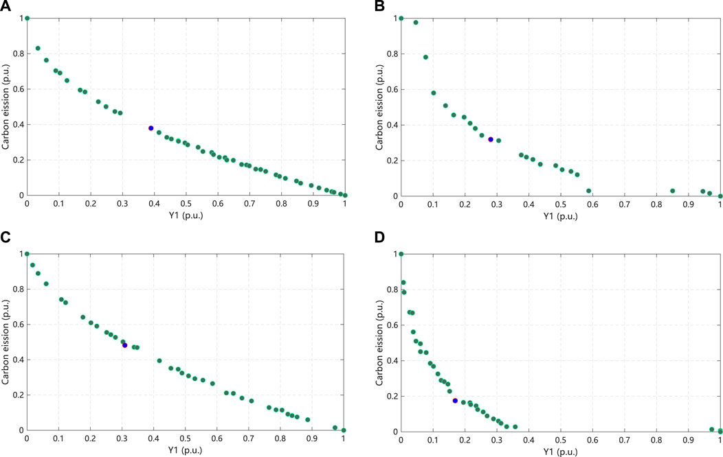
Figure 6. Two-dimensional schematic of the multi-objective Pareto surface for the first quarter: (A) Model 1, (B) Model 2, (C) Model 3, and (D) Model 4.

In order to show more intuitively the multi-objective presentation of the four different types of energy-intensive enterprises in each quarter, Figures 7–10 present the three-dimensional schematic multi-objective Pareto surfaces of the 24-hour continuous production plants, the day-only production plants, the night-only production plants, and the eco-peak production plants in the quarter, respectively.

Figure 7

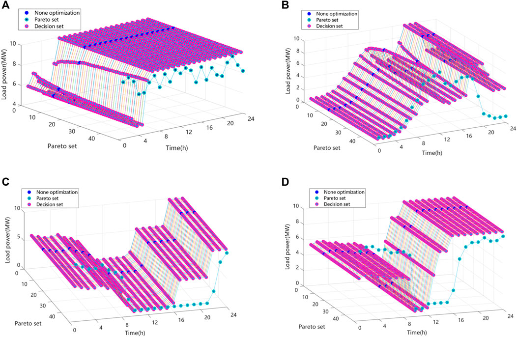
Figure 7. Three-dimensional schematic of the multi-objective Pareto surface for a 24-h continuous production plant in one-quarter: (A) Model 1, (B) Model 2, (C) Model 3, and (D) Model 4.

Figure 8

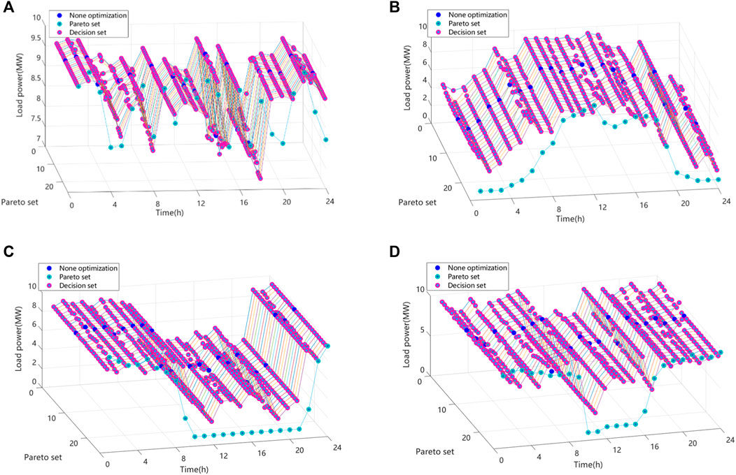
Figure 8. Three-dimensional schematic of the multi-objective Pareto surface for a pure daytime production plant in one-quarter: (A) Model 1, (B) Model 2, (C) Model 3, (D) Model 4.

Figure 9

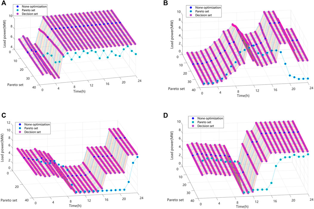
Figure 9. Three-dimensional schematic of the multi-objective Pareto surface for a pure nighttime production plant in one-quarter: (A) Model 1, (B) Model 2, (C) Model 3, and (D) Model 4.

Figure 10

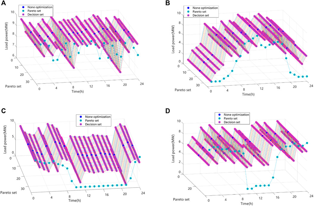
Figure 10. Three-dimensional schematic of the multi-objective Pareto surface for an environmental protection staggered production plant in one-quarter: (A) Model 1, (B) Model 2, (C) Model 3, and (D) Model 4.

The ideal point decision is used to find the optimal solution among carbon emissions, electricity costs, and electricity losses.

Tables 2–5 show the electricity cost, carbon emissions, peaking cost, and user comfort of each high-energy-consuming enterprise in all seasons of the year, and the results screened by the genetic algorithm and the interior point method with the ideal point decision are compared with the values before optimization using each measure as a single objective.

Table 2

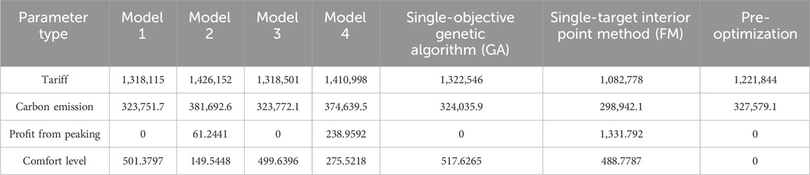
Table 2. Comparison of before and after optimization of each objective in the first quarter.

Table 3

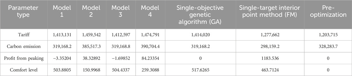
Table 3. Comparison of before and after optimization of each objective in the second quarter.

Table 4

Table 4. Comparison of before and after optimization of each objective in the third quarter.

Table 5

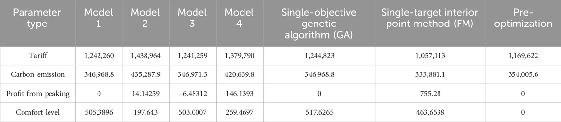
Table 5. Comparison of before and after optimization of each objective in the fourth quarter.

Table 6 shows the cost of electricity for different energy-consuming enterprises in different quarters, combining the electricity tariffs and peaking costs to obtain more realistic data, which visually shows the cost of large amounts of electricity used by different production methods in different time periods. Electricity tariffs are the basic fees that companies pay to the power company for the amount of electricity they use, while peaking costs are the costs of using electricity during peak hours of the power system. Electricity systems often impose an additional charge on businesses that use electricity during peak hours, which is intended to encourage businesses to use less electricity during peak hours in order to balance the load on the power system.

Table 6

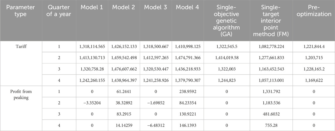
Table 6. Analysis of electricity costs.

From the above table, it can be seen that the electricity consumption of the 24-h continuous production type factory is slightly higher than before the optimization, and the comfort level of electricity consumption has improved. When comparing the purely daytime production type factory with the purely nighttime production type factory, it is obvious that the former has a higher cost of electricity consumption, which is 10,000 yuan higher than the latter on average. The cost of electricity use is higher during the peak hours of the day. This also reflects the variability of electricity costs across time, and firms may need to consider energy efficiency measures during peak hours. The electricity cost spent by the eco-peak production type of factory is closer to that of the night-only production type of factory. This suggests that the eco-peak production type of factory has been relatively optimized in terms of energy use and has relatively lower electricity costs but still maintains a degree of production flexibility.

5 Conclusion

In conclusion, the work in this paper includes the following innovations:

1) An optimization model of the electricity consumption behavior of power consumers driven by a dynamic electro-carbon factor is developed. It not only analyzes the electricity consumption behavior of high-energy-consuming enterprises but also incorporates the peaking cost at the cost of electricity consumption while not sacrificing the comfort of the enterprise’s electricity consumption as much as possible to provide meaningful guidance for the enterprise’s energy saving and emission reduction.

2) This paper simulates and analyses the electricity consumption behavior of energy-consuming enterprises with different production modes and compares the annual electricity consumption of environmentally friendly staggered-peak production factories with that of purely daytime production factories, purely nighttime production factories, and 24-h production factories in order to encourage business users to analyze and study the above conclusions, motivate them to take energy-saving measures during peak electricity consumption periods as far as possible, try to stagger their production to safeguard their own electricity consumption while reducing their expenditure on electricity consumption and carbon emissions, and contribute to the reduction of carbon emissions.

Data availability statement

The original contributions presented in the study are included in the article/supplementary material; further inquiries can be directed to the corresponding author.

Author contributions

YY: funding acquisition, investigation, methodology, writing–original draft, and writing–review and editing. FP: conceptualization, data curation, formal analysis, writing–original draft, and writing–review and editing. JL: project administration, resources, and writing–original draft. YJ: software, supervision, writing–review and editing, and conceptualization. LZ: validation, visualization, and writing–original draft. JZ: conceptualization, data curation, formal analysis, and writing–review and editing.

Funding

The author(s) declare that financial support was received for the research, authorship, and/or publication of this article. This work was jointly supported by the National Key Research and Development Program of China (2022YFF0606600) and the Science and Technology Project of China Southern Power Grid (GDKJXM20230256).

Conflict of interest

Authors YY, FP, JL, YJ, LZ, and JZ were employed by Metrology Center of Guangdong Power Grid Co., Ltd. The authors declare that this study received funding from China Southern Power Grid. The funder had the following involvement in the study: Study design.

Publisher’s note

All claims expressed in this article are solely those of the authors and do not necessarily represent those of their affiliated organizations, or those of the publisher, the editors, and the reviewers. Any product that may be evaluated in this article, or claim that may be made by its manufacturer, is not guaranteed or endorsed by the publisher.

References

Abbasi, K. R., and Adedoyin, F. F. (2021). Do energy use and economic policy uncertainty affect CO 2 emissions in China? Empirical evidence from the dynamic ARDL simulation approach. Environ. Sci. Pollut. Res. 28, 23323–23335. doi:10.1007/s11356-020-12217-6

CrossRef Full Text | Google Scholar

Abbasi, K. R., Shahbaz, M., Jiao, Z., and Tufail, M. (2021). How energy consumption, industrial growth, urbanization, and CO2 emissions affect economic growth in Pakistan? A novel dynamic ARDL simulations approach. Energy 221, 119793. doi:10.1016/j.energy.2021.119793

CrossRef Full Text | Google Scholar

Boyaci, O., Umunnakwe, A., Sahu, A., Narimani, M. R., Ismail, M., Davis, K. R., et al. (2022). Graph neural networks based detection of stealth false data injection attacks in smart grids. IEEE Syst. J. 16, 2946–2957. doi:10.1109/JSYST.2021.3109082

CrossRef Full Text | Google Scholar

Grygar, D., and Fabricius, R. (2019). An efficient adjustment of genetic algorithm for Pareto front determination. Transp. Res. Procedia 40, 1335–1342. doi:10.1016/j.trpro.2019.07.185

CrossRef Full Text | Google Scholar

Hancer, E., Xue, B., Zhang, M., Karaboga, D., and Akay, B. (2018). Pareto front feature selection based on artificial bee colony optimization. Inf. Sci. 422, 462–479. doi:10.1016/j.ins.2017.09.028

CrossRef Full Text | Google Scholar

Huebner, G., Shipworth, D., Hamilton, I., Chalabi, Z., and Oreszczyn, T. (2016). Understanding electricity consumption: a comparative contribution of building factors, socio-demographics, appliances, behaviours and attitudes. Appl. energy 177, 692–702. doi:10.1016/j.apenergy.2016.04.075

CrossRef Full Text | Google Scholar

Huwei, W., Shuai, C., and Chien-Chiang, L. (2023). Impact of low-carbon city construction on financing, investment, and total factor productivity of energy-intensive enterprises. Energy J. 44 (2), 79–102. doi:10.5547/01956574.44.2.hwen

CrossRef Full Text | Google Scholar

Laicane, I., Blumberga, D., Blumberga, A., and Rosa, M. (2015). Evaluation of household electricity savings. Analysis of household electricity demand profile and user activities. Energy Procedia 72, 285–292. doi:10.1016/j.egypro.2015.06.041

CrossRef Full Text | Google Scholar

Lin, B., and Jia, Z. (2020). Economic, energy and environmental impact of coal-to-electricity policy in China: a dynamic recursive CGE study. Sci. Total Environ. 698, 134241. doi:10.1016/j.scitotenv.2019.134241

PubMed Abstract | CrossRef Full Text | Google Scholar

Liu, S., Wu, C., and Zhu, H. (2022). Topology-aware graph neural networks for learning feasible and adaptive AC-OPF solutions. IEEE Trans. Power Syst. 38, 5660–5670. doi:10.1109/tpwrs.2022.3230555

CrossRef Full Text | Google Scholar

Liu, Y., Xie, H., Presekal, A., Stefanov, A., and Palensky, P. (2023). A GNN-based generative model for generating synthetic cyber-physical power system topology. IEEE Trans. Smart Grid 14, 4968–4971. doi:10.1109/TSG.2023.3304134

CrossRef Full Text | Google Scholar

Martinez-Gil, J., Freudenthaler, B., and Natschlaeger, T. (2013). “Modeling user behavior through electricity consumption patterns,” in 2013 24th International Workshop on Database and Expert Systems Applications, Los Alamitos, CA, USA, 26-30 August 2013 (IEEE), 204–208.

CrossRef Full Text | Google Scholar

Papachristos, G. (2015). Household electricity consumption and CO2 emissions in The Netherlands: a model-based analysis. Energy Build. 86, 403–414. doi:10.1016/j.enbuild.2014.09.077

CrossRef Full Text | Google Scholar

Ruhnau, O., Bucksteeg, M., Ritter, D., Schmitz, R., Böttger, D., Koch, M., et al. (2022). Why electricity market models yield different results: carbon pricing in a model-comparison experiment. Renew. Sustain. Energy Rev. 153, 111701. doi:10.1016/j.rser.2021.111701

CrossRef Full Text | Google Scholar

Saint Akadiri, S., Alola, A. A., Olasehinde-Williams, G., and Udom Etokakpan, M. (2020). The role of electricity consumption, globalization and economic growth in carbon dioxide emissions and its implications for environmental sustainability targets. Sci. Total Environ. 708, 134653. doi:10.1016/j.scitotenv.2019.134653

PubMed Abstract | CrossRef Full Text | Google Scholar

Stedmon, A. W., Winslow, R., and Langley, A. (2013). Micro-generation schemes: user behaviours and attitudes towards energy consumption. Ergonomics 56 (3), 440–450. doi:10.1080/00140139.2012.723140

PubMed Abstract | CrossRef Full Text | Google Scholar

Sun, W., and Huang, C. (2022). Predictions of carbon emission intensity based on factor analysis and an improved extreme learning machine from the perspective of carbon emission efficiency. J. Clean. Prod. 338, 130414. doi:10.1016/j.jclepro.2022.130414

CrossRef Full Text | Google Scholar

Suzuki, S., Takeno, S., Tamura, T., et al. (2020). Multi-objective Bayesian optimization using Pareto-frontier entropy. PMLR 119, 9279–9288.

Google Scholar

White, K., Habib, R., and Hardisty, D. J. (2019). How to SHIFT consumer behaviors to be more sustainable: a literature review and guiding framework. J. Mark. 83 (3), 22–49. doi:10.1177/0022242919825649

CrossRef Full Text | Google Scholar

Xiao, H., Gan, H., Yang, P., Li, L., Hao, Q., et al. (2023b). Robust submodule fault management in modular multilevel converters with nearest level modulation for uninterrupted power transmission. IEEE Trans. Power Deliv. 99, 1–16. doi:10.1109/TPWRD.2023.3343693

CrossRef Full Text | Google Scholar

Xiao, H., He, H., Zhang, L., and Liu, T. (2023a). Adaptive grid-synchronization based grid-forming control for voltage source converters. IEEE Trans. Power Syst. 99, 4763–4766. doi:10.1109/TPWRS.2023.3338967

CrossRef Full Text | Google Scholar

Yan, X., He, Y., and Fan, A. (2023). Carbon footprint prediction considering the evolution of alternative fuels and cargo: a case study of Yangtze river ships. Renew. Sustain. Energy Rev. 173, 113068. doi:10.1016/j.rser.2022.113068

CrossRef Full Text | Google Scholar

Zeng, Q., Shi, C., Zhu, W., Zhi, J., and Na, X. (2023b). Sequential data-driven carbon peaking path simulation research of the Yangtze River Delta urban agglomeration based on semantic mining and heuristic algorithm optimization. Energy 285, 129415. doi:10.1016/j.energy.2023.129415

CrossRef Full Text | Google Scholar

Zeng, X., Zhang, Y., Guo, B., Huang, L., and Li, C. (2023a). “Optimal day-ahead dispatch of air-conditioning load under dynamic carbon emission factors,” in IEEE Conference Publication, Chengdu, China, 23-26 March 2023 (IEEE).

CrossRef Full Text | Google Scholar

Zhang, X., Gan, D., Wang, Y., Liu, Y., Ge, J., and Xie, R. (2020). The impact of price and revenue floors on carbon emission reduction investment by coal-fired power plants. Technol. Forecast. Soc. Change 154, 119961. doi:10.1016/j.techfore.2020.119961

CrossRef Full Text | Google Scholar

Zhang, X., Guo, Z., Pan, F., Yang, Y., and Li, C. (2023). Dynamic carbon emission factor based interactive control of distribution network by a generalized regression neural network assisted optimization. Energy 283, 129132. doi:10.1016/j.energy.2023.129132

CrossRef Full Text | Google Scholar