Enhanced harris hawks optimization based load frequency control of multi area microgrid based water treatment plant with consideration of 3DOF-(FO-PIDN)/(TIDN) controller

1 Introduction

In some cases, industrial plants such as water treatment facilities may not be connected to the main electrical grid and must rely on conventional Diesel Engine Generators (DEG) during power outages (Rohmingtluanga et al., 2022; Rohmingtluanga et al., 2023). However, the use of DEG alone is known to be expensive and contribute to greenhouse gas emissions. As a result, renewable energy sources (RES) have become a primary focus for reducing greenhouse gas emissions and conserving energy (Wentzel et al., 2012). Nevertheless, combining RES with existing DEG systems can be a complicated process, requiring advanced control and other reliable system such as energy storage systems to optimize for their intermittency. Additionally, strategies for complex control is required to affirm stable operation, especially for critical loads like water treatment facilities (Tchobanoglus et al., 2003; Baghaee et al., 2017). One effective method of integrating RES generation into the electric power system is through the use of microgrid systems (Zhang et al., 2016; Latif et al., 2020). A microgrid system is a small-scale power system that includes energy sources, interconnected loads, and energy storage systems (ESSs) within a defined electrical area. It can be operated in either a grid-connected or islanded mode (Sreedharan et al., 2016), where the voltage and frequency variations in grid-connected mode are controlled by the utility grid, while regulation in islanded mode is achieved through solar and wind energy compensation (Kikusato et al., 2022). Moreover, a novel concept of a multi-microgrid (MMG) system has been introduced, which consists of multiple interconnected microgrids for mutual power supply (He et al., 2017). In a microgrid system, reliable operation is ensured through three levels of hierarchical control: primary, secondary, and tertiary control. A conventional method (the primary droop control), is responsible for maintaining the microgrid voltage and frequency in islanded mode, enabling the DGs to share reactive and active power with no links of communication. However, this may result in frequency deviation (Dey et al., 2020).

The fluctuating and unreliable power production of RESs can lead to an imbalance between power generation and demand, causing frequency disturbance and threatening grid security (Chakraborty et al., 2022). Maintaining a desirable range of load frequency is therefore a major task for power engineers. Load frequency control (LFC) aims to regulate system frequency while consuming fewer fuels and increasing battery lifetime (Babazadeh and Karimi, 2013). The Load Frequency Control (LFC) plays an important function in power systems since it not only reduces frequency deviation to zero in the case of a system disruption, but it also guarantees that the power transferred on the tie-line among linked power systems remains at the value used as a reference (Barik et al., 2021). Therefore, the use of energy storage systems (ESSs) is considered as one of the best solutions to ensure the quality and reliability of the power system (Abdolrasol et al., 2021). Because of its low daily self-discharge rate, quick reaction time, and high cycle efficiency, rechargeable battery packs are widely used in independent power systems (Li et al., 2008). To improve the response of Load Frequency Control (LFC) on the DGs of islanded MG, several controllers such as ordinary PID control, smart control, adaptable control, resilient control, and MPC control have been used (Chauhan et al., 2021). The existing controllers for Load Frequency Control (LFC) are found to be inadequate. Therefore, in order to maintain load frequency within the nominal value, a PID controller based on the EHHO approach is proposed in this paper. The proposed controller is designed specifically for a multi-microgrid-based water treatment plant.

The focus of this paper is to address frequency issues and deviations, which are commonly observed in existing power systems as well as in multi-area microgrid systems. To control the frequency at the desired value, the study proposed an Enhanced Harris Hawks Optimization Algorithm (EHHO)-based PID controller. The controller considered SPV, small hydro (SHG), BESS, and DEG as power sources for peak demand. The proposed controller was implemented in MATLAB, and its performance was analysed and compared with existing techniques such as PSO and GWO. This paper also aims to improve the performance of the system and comprehension by introducing various controllers, including PID, 3DOF-FOPIDN, and 3DOF-TIDN, and optimizing their parameters through PSO algorithm. Additionally, the study conducts stability and robustness analyses.

Based on the above, the main contribution of this paper are as follows:

1) Working on energy-water, nexus, it considers each pumping station as a three-area WTP based microgrid system.

2) To implement various DGs such as solar, wind Battery and Diesel engine on each pumping stations of the microgrid system

3) To adapt and apply Enhanced Harris Hawks Optimization Technique and compare the performance with conventional optimization techniques

4) To implement 3DOF-FOPIDN, 3DOF-TIDN controller and compare the performance with conventional controller

5) To perform stability and robustness analysis of the proposed controller

This study highlights the importance of incorporating advanced control systems into critical water and energy infrastructure. This aligns with the increasing recognition of these sectors as crucial components in various jurisdictions, such as the European Union’s NIS 2 Directive.

The rest of the paper is organized as followed: Section-2 discussed the mathematical modelling of the proposed system, Section-3 highlights the frequency controller (fc), Section-4 discussed PID controller and various optimization techniques, tuning optimal parameters of PID controller using EHHO is discussed in Section-5. Analysis of the proposed controller is highlighted in section-6, in section-7 Implementation of proposed controllers such as 3DOF-FOPIDN and 3DOFTIDN controllers is discussed and Section-8 discussed Stability analysis and Robustness analysis. Lastly the paper is concluded in Section-9.

2 Mathematical modelling

2.1 Wind turbine generator

Wind turbines are typically used to harness kinetic energy derived from wind and convert it into mechanical energy (Yammani and Maheswarapu, 2019). This mechanical energy is subsequently transmitted to the generator’s rotor through a shaft, and the generator converts the mechanical energy into electrical energy. The mathematical representation of the mechanical output of a wind turbine is shown in Equation 1.

$P_T=\frac{1}{2}\rho A{C}_P\left(\lambda ,\beta \right)V_{\omega }^3(1)$

where, P_m represents mechanical power derived from the rotor shaft, P_w is the power of wind content in the virtual stream tube consisting Wind turbine (Karimi et al., 2016). Figure 1A represents the WTG first-order transfer function block.

Figure 1

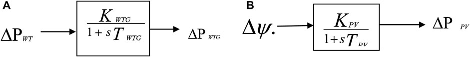
Figure 1. (A) WTG first-order transfer function block, (B) SPV power’s first-order transfer function model.

2.2 Photo Voltaic cells

A SPV system is a power generation system that converts sunlight directly into electricity, and can be used for both grid-connected mode and standalone. The increasing popularity of SPV systems in current years can be attributed to government policies that encourage their use, the increased demand for power, concerns regarding the environment, cheap operational costs, and the lack of fuel expenses. The amount of power output from a SPV system is dependent on the solar irradiance, ambient temperature, and the conversion efficiency of the SPV panel (Obaid et al., 2019). SPV power output (W) can be given as,

$\stackrel{pv}{P}\left(s\left(t\right)\right)={\eta }_{cells}*FF*V*I(2)$

Similarly, the terminal voltage can be given as,

$V=V_{oc}+K_{vt}*T_{ct}(3)$

Also, the fill factor is given as,

$FF=\frac{V_{mp}*I_{mp}}{V_{oc}*I_{sc}}(4)$

Where, V_mp is the voltage at maximum power in V, I_mp is the current at maximum power in A, V_oc is the open-circuit voltage in V, K_vt is the voltage temperature coefficient in mV/°C, where, η_cells is the number of SPV cells.

Similarly, the current (A) is given as,

$I=s\left(t\right)*\left[I_{sc}+K_{ct}*\left(T_{ct}-25\right)\right](5)$

Where, I_sc is the short-circuit current in A, K_ct is the current temperature coefficient in mA/°C, T_at is the ambient temperature in °C, s(t) is the random irradiance, NOCT is the nominal cell operating temperature in °C.

The cell temperature in °C is given as,

$T_{ct}=T_{at}+s\left(t\right)*\left[\frac{NOCT-20}{0.8}\right](6)$

The SPV power’s first-order transfer function model is given in Figure 1B.

2.3 Diesel engine generator

Diesel generators are a common component in power systems that are used to meet the electricity needs of consumers. These generators offer reliable and long-lasting power solutions for applications ranging from prime power to standby power. Diesel generators are used as backup power sources, emergency and reserve, etc. due to its unique features such as availability, rapid start-up, consistency, robustness, and black start ability (Zhang et al., 2017). Despite some drawbacks, these features make diesel generators a popular choice in certain locations. The rate of fuel consumption of a diesel generator at any given time t is directly related to its output power, and can be represented mathematically.

$F=F_0.Y_{dg}+F_1.P_{dg}(7)$

Where, F₀ is the fuel curve intercept coefficient (units/h/kW), F₁ is the fuel curve slope (units/h/kW), P_dg is the electrical output of the generator (kW) and Y_dg is the rated capacity of the generator (kW).

The DEG model of the first-order transfer function block is represented in Figure 2A shown below. Using the governor control action DEG maintains the equilibrium between demand for electricity and production in an independent microgrid owing to variations in solar and wind power.

Figure 2

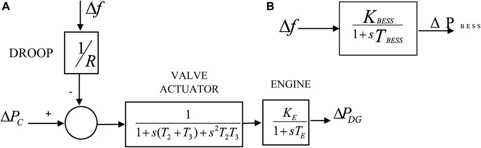
Figure 2. (A) DEGs transfer function first order block, (B) the BESS transfer function first-order block.

2.4 Battery energy storage system model

BESS are frequently employed for enhancing autonomous MG’s primary frequency control. DEG is often in charge of the principal frequency control duty. DEGs, on the other hand, have a prolonged time constant and gradual respond to frequency fluctuations, which can result in significant overshoot (Adefarati et al., 2017). BESS can be added into the system to solve this issue and improve the primary frequency response. The state of charge of BESS at any time t, as well as the limits state of charge of the BESS as a function of optimal BESS capacity $\underset{bess}{\overset{cap}{ESS}}$, are calculated as follows:

$SOC\left(t\right)=SOC\left(t-1\right)\left(1-S_{bess}\right)+\underset{bess}{\overset{ch}{P}}\left(t\right)*\underset{bess}{\overset{c}{\eta }}-\frac{\underset{bess}{\overset{dis}{P}}\left(t\right)}{\underset{bess}{\overset{d}{\eta }}}(8)$

${SOC}_{bess}^{\min }=0.2*{ESS}_{bess}^{cap}(9)$

${SOC}_{ptes}^{\max }=0.8*{ESS}_{bess}^{cap}(10)$

Where, the present and earlier energy capacity of the BESS are represented as SOC (t) and SOC (t-1) over one-time step and the rate of self-discharge is represented as $\stackrel{bess}{S}$. The BESS charging and discharging of power are represented as $\underset{bess}{\overset{ch}{P}}$ and $\underset{bess}{\overset{dis}{P}}$ which are the characteristics of the electric power supply system’s surpluses and shortfalls, correspondingly. $\underset{bess}{\overset{c}{\eta }}$ and $\underset{bess}{\overset{d}{\eta }}$ are the BESS discharging and charging efficiencies.

The BESS transfer function first-order block is given in Figure 2B. Also, negative of ΔF represents Discharging and positive of ΔF represents Charging of the BESS with respect to the system frequency.

3 Frequency controller (FC)

Before implementing controller design for an optimization technique, it is important to establish the fitness function. There are several performance indices that are commonly used in design of the controller. In this paper, the fitness function used is the integral time absolute error (ITAE), as presented in Eq. 11 for interconnected multi area microgrid unit (Hossain et al., 2019). Despite load disturbances, the goal is to achieve practically zero deviation in frequency and tie-line power flow fluctuations.

ITAE criteria are used as the fitness function in this work to fine-tune the PID controller gains. Because ITAE creates lower overshoots/undershoots as well as fluctuations, it is recommended over other performance indices. ISE, on the other hand, has a reduced overshoot as well as a longer settling time, IAE has a slower reaction than ISE in design of Load frequency controller, and ITSE has a bigger controller response for abrupt changes in supply. Eq. 11 defines the fitness function ITAE, whereas Eq. 12 defines the PID controller’s gain bounds.

Fitness = Minimize {ITAE}

$=\mathit{Min}\left\{{\displaystyle \underset{0}{\overset{T}{\int }}}\left(\left|\Delta \left.F_i\right|\right.+\left|\Delta \left.P_{tie-line,ij}\right|\right.\right)\dots t.dt\right\}(11)$

Subjected to PID gain limits,

$\left.\begin{array}{c}\underset{p}{\overset{\min }{K}}\le K_p\le \underset{p}{\overset{\max }{K}}\\ \underset{i}{\overset{\min }{K}}\le K_i\le \underset{i}{\overset{\max }{K}}\\ \underset{d}{\overset{\min }{K}}\le K_d\le \underset{d}{\overset{\max }{K}}\end{array}\right\}(12)$

The variables i and j are being utilized in this context to denote area numbers. More specifically, i is limited to the values 1, 2, and 3 while j is restricted to 2 and 3. Additionally, it should be noted that i and j cannot be equivalent (i.e., i is not equal to j). Furthermore, the terms “min” and “max” are being employed to represent the lowest and highest values of various parameters of the controllers.

The regulation of frequency deviation is commonly achieved by utilizing PID controllers. However, it is frequently seen that the PID controller performance in regulating frequency deviation is insufficient to achieve the desired level of accuracy (Mishra et al., 2020). Therefore, the parameters of the PID controller such as K_p, K_i, and K_d are adjusted appropriately to enhance its performance in regulating frequency deviation. Therefore, in this paper, a technique-based PID controller has been introduced and tuned using the EHHO technique to regulate frequency deviation.

4 Optimization techniques

4.1 PSO optimization

Kennedy and Eberhart introduced the PSO algorithm as an evolutionary optimization technique, inspired by animal social behaviors, such as the movement of schools of fish or flocks of birds, in finding food and avoiding predators. These creatures possess remarkable traits that are functional and have been optimized through many iterations of a vast optimization algorithm in the DNA of living beings (Nayak et al., 2023). Consequently, the PSO Algorithm, like other intelligent optimization algorithms, is influenced by nature. The algorithm employs random numbers and is structured in the following way:

The PSO algorithm can be broken down into six steps. The first step is the initialization of the population, which creates a random number to serve as the starting location for each particle or sequence’s motif candidate. Step 2 calculates the fitness value for each particle, and parameter pBest stores the particle with the highest fitness value. In Step 3, the global maximum fitness value (gBest) is updated. Step 4 involves calculating velocities using a randomization approach. In Step 5, each particle’s new location is updated using a velocity value. Finally, Step 6 pertains to the termination condition, where the process flow is terminated if the condition is satisfied. Otherwise, the process flow will be repeated from Step 2.

4.2 GWO optimization

Grey wolves are known to be highly skilled predators that excel at locating prey. Their social hierarchy, as depicted in Figure 3A, is a fascinating characteristic of these animals. The group is organized into a rigid dominating structure, with the most powerful member of the pack being the Alpha, which can be either male or female. The Alpha wolf makes critical decisions about hunting, migration, sleeping locations, and eating (Ulutas et al., 2020).

Figure 3

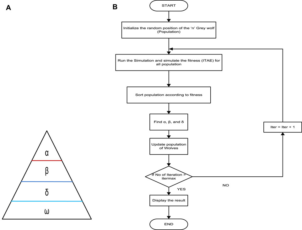
Figure 3. (A) GWO hierarchy (B) Flow chart of GWO algorithm.

The Alpha wolf is not necessarily the strongest member of the group but must be the best at controlling the pack, emphasizing that dedication and society are more significant than power. The beta wolf is the next level in the hierarchy, and they assist the Alpha wolf in making decisions. When the Alpha wolf becomes ill or dies, the beta wolf takes over as the leader. The beta wolf also serves as the disciplinarian and counsellor to the Alpha wolf. Delta, the third level in the hierarchy, is dominant in omega but must report to the Alpha and beta wolves. Scouts, carers, and hunters fall within the delta category. Omega is at the bottom of the hierarchy and is made the scapegoat, allowing them to eat last. These wolves’ absence can lead to internal strife and issues within the group. The GWO flow chart, shown in Figure 3B, follows this hierarchical structure (Gheisarnejad and Khooban, 2019).

5 Optimal tuning of PID controller parameters using EHHO

An effective EHHO control strategy is presented in this section for the regulation of load frequency deviation in MG environment. The operation of PID controller is enhanced by optimally tuning the PID parameters, including K_p, K_d, and K_i. To accomplish this, EHHO is utilized to obtain the required values for these parameters.

HHO algorithm is inspired by the hunting behavior of the Harris’s hawks. The HHO algorithm is designed to mimic the surprise pounce technique used by Harris’s hawks to catch prey. The hawks cooperate and chase from random positions and surprise its prey. This algorithm is preferred due to its simplicity and low number of control parameters (Vafamand et al., 2019). The proposed EHHO approach uses the PSO to boost the behavior of the conventional HHO by improving the updating process. The operation of EHHO is described in detail.

5.1 Exploration phase

In nature, Harris’s hawks use their powerful eyes to locate and identify their prey, but sometimes, the prey may not be easily visible. Therefore, the hawks perch, observe, and monitor the desert area for several hours to detect a potential prey. In HHO, the candidate solutions are considered as the hawks, and the finest results in each iteration is measured as the target or the ideal prey. The hawks randomly perch on various places and pauses to sight a target using two approaches. Firstly, they perched along other family members of various locations (to attack the prey while being close to each other), and the prey, which is represented by Eq. 13 when j < 0.5. Alternatively, they perch on tall trees randomly located within the group’s home range, as shown in Equation (6 and (14) when j ≥ 0.5.

$P\left(s+1\right)=\left\{\begin{array}{ll}{p}_{rand}\left(s\right)-x_1\left|P_{rand}\left(S\right)-2x_{2}P\left(S\right)\right|& j\ge 0.5\\ \left(P_{rabbit}-P_m\left(s\right)\right)-x_3\left(lb+x_4\left(ub-lb\right)\right)& j〈0.5\end{array}\right.(13)$

From the above, $P_{rand}\left(s\right)$ is a randomly selected hawk, $P\left(s+1\right)$ is the vector of hawks position in the consecutive iteration s, $P_{rabbit}\left(s\right)$ represents rabbit (prey) location, $P\left(s\right)$ is the vector of present hawks position, x₁, x₂, x₃, x₄ and j (random numbers) are updated in each iteration and are within (0,1), and $P_m$ is the position of the present hawks, u_b is the upper bounds and l_b is the lower bounds variables,. The normal position of the hawks is shown in (14).

$P_m\left(s\right)=\frac{1}{n}{\displaystyle \sum _{i=1}^n}{P}_i\left(s\right)(14)$

Where, s and n represent the total hawks and $P_i\left(s\right)$ represents the iteration location of each hawk and Eq. 11 is used to calculate the fitness function.

5.2 Transition from exploration to exploitation

The energy of the prey reduces significantly during its escape behavior, and this is reflected in the prey’s energy equation. as below:

$E=E_0\left(1-\frac{t}{S}\right)(15)$

The energy of a prey is given by equation E, where E_o is the initial energy, t is the iteration, S is the iteration maximum number. As the prey’s energy decreases during the escaping behavior, it becomes less likely to escape. Hence, the hawks adopt different strategies depending on the prey’s energy and distance. Exploitation involves besiege of hard and soft with landing dives, while exploration involves searching particles average locations.

5.3 Exploitation phase

The hawks done a rapid dive on the prey previously detected in the iteration phase and the prey normally try to avoid danger, and the chasing behavior of hawks varies in response to different escaping behaviors. To model the attacking stage in HHO, four possible strategies are proposed as shown in the below Table 1.

Table 1

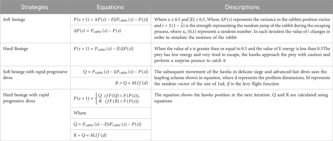
Table 1. Strategies of HHO Exploitation phase.

The HHO algorithm has two strategies to attack prey: soft besiege and hard besiege. The hard besiege has similar characteristics to the soft besiege, but its Q and R conditions are different. To visualize the HHO tracking, the vector addition structure is used and shown in Figure 4A. Additionally, the flow chart of the HHO algorithm is illustrated in Figure 4B.

Figure 4

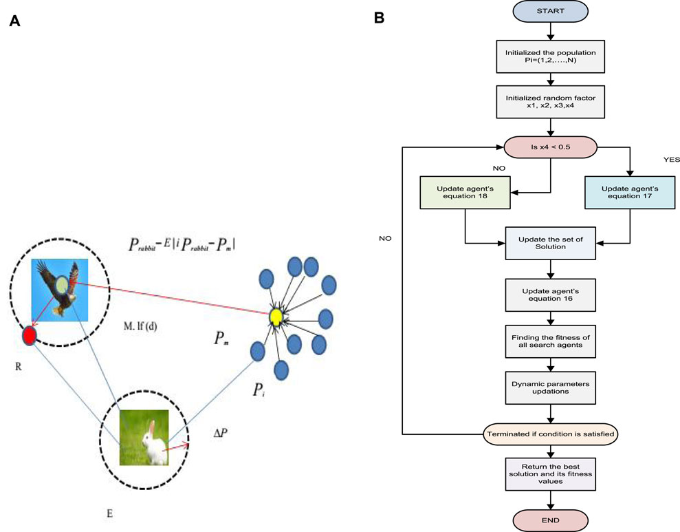
Figure 4. (A) Visualization of HHO tracking with vector addition (B). Flow chart of HHO algorithm.

In order to improve the efficiency of the conventional HHO algorithm, an enhancement is proposed by integrating the velocity updating equation of the PSO algorithm into the updating process of HHO.

$V_{id}=V_{id}+C{1}^{*}rand{\left(\right)}^{*}\left(P_{id}-X_{id}\right)+c{2}^{*}rand{\left(\right)}^{*}\left(P_{gd}-X_{id}\right)(16)$

Where, V_id is the velocity of the hawk; X_id is the present hawk position. P_id and P_gd shows pbest and gbest. rand () is a random number inside (0,1). cL, c2 are learning factors. Normally used as c₁ = c₂ = 2.

6 Analysis

Performance analysis of the EHHO control scheme is done for controlling frequency deviation in RES-based proposed WTP based microgrids. The proposed LFC comprises various renewable energy sources, including SPV, WTG, BESS, and DEG, and considers three microgrid systems for each pumping station with tie line connections. The proposed technique is implemented using MATLAB platform and its performance is evaluated. To evaluate the frequency control performance of the proposed EHHO-based PID controller, we compare it with other existing methods, such as GWO and PSO. Figure 5 shows the proposed system simulink diagram.

Figure 5

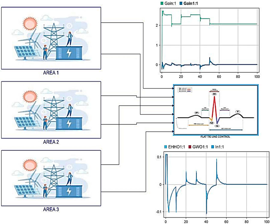
Figure 5. Proposed system simulink diagram.

6.1 PSO based controller

In this sub section, PSO based controller performance is discussed separately for each area of the microgrid sections considering WTP. The values are derived from PSO based multi-microgrid system. The performance of PSO based controller for SPV, WTG, BESS, DEG, load deviation and frequency deviation for each unit as well as tie line within each area is shown in the following figures separately as shown below. The PSO based controller has attained the average output power of SPV and WTG as 0.25 p. u. and 0.36 p. u. respectively. Similarly, the response of BESS and DEG are shown in the figure. The PSO based controller has attained the load deviation between 1.25 p. u to almost 2.1 p. u.Also, the PSO based controller performance for frequency deviation has been attained almost zero value with high deviation.

6.1.1 Microgrid area-1

The performance of different power sources and load of Microgrid area-1 under PSO is shown below. Figure 6A shows load deviation in pu. Figure 6B shows output power of BESS and Diesel Engine Generator, Similarly, Figure 6C shows frequency deviation of area 1 in Hz, also, Figure 6D shows the total output power of area-1 in P.U. and Figure 6E represents frequency deviation of area-2 in Hz.

Figure 6

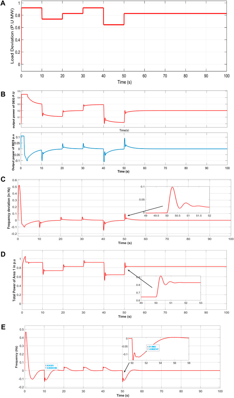
Figure 6. (A) Load Deviation frequency deviation, (B) Output power of DEG and BESS, (C) Frequency deviation of area-1 in Hz, (D) Output power of area-1 in pu, (E) Frequency deviation of area-2 in Hz.

6.1.2 Microgrid Area-2 and area-3

Similar to area-1 The performance of different power sources and load of Microgrid area-2 under Particle Swarm Optimization PSO is shown in the figures. Figure 7A shows the total output power of area-2 in P.U. Similar to area-1 and area-2, the performance of Microgrid area-3 under PSO is shown in the following figures. Figure 7B shows frequency deviation of area 3 in Hz, also, Figure 7C shows the total output power of area-3 in pu.

Figure 7

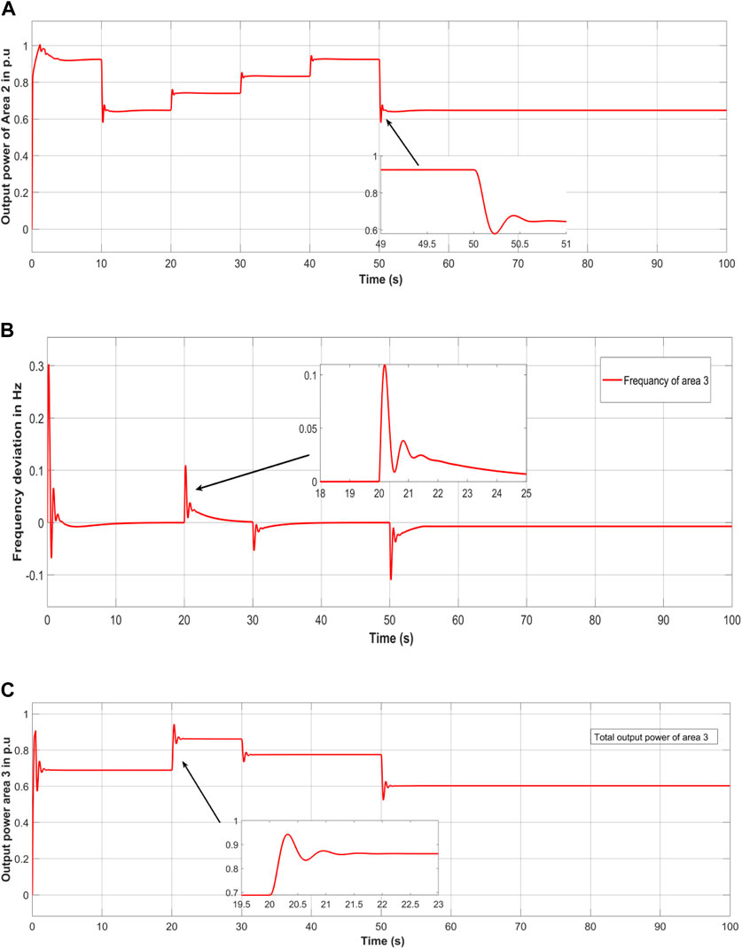
Figure 7. (A) total output power of area-2 in pu, (B) Frequency deviation of area-3 in Hz. (C) Total output power of area-3 in pu.

6.2 Tie line values under PSO

The performance of the tie line values such as frequency deviation and power of each of the Microgrid area −1, −2 and −3 under PSO is shown in the following figures. Figure 8 shows the tie line power deviation of each Microgrid such as (a) area-1 and area-2 (b) area 2 and 3 (c) area-1 and area-3. Similarly, the iteration for fitness function convergence of PSO is shown in Figure 8D showing that at 50 iteration the PSO shows best convergence result.

Figure 8

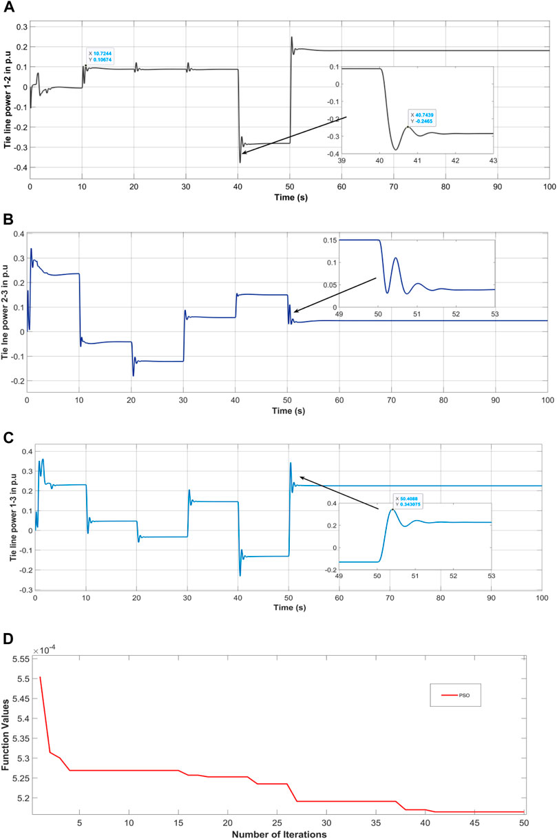
Figure 8. Tie line power deviation (A) area-1 and area-2, (B) area −2 and area-3 (C) area-1 and area-3, (D) convergence plot of PSO.

6.3 Comparative analysis

In this section the performance of the proposed controller and existing controllers such as PSO, GWO and EHHO based controller is compared and evaluated in this sub section. The comparative performance of the proposed and existing controller for each microgrid areas are shown and explained in the following sub sections. The following Table 2 shows the optimized controller parameters with different algorithms.

Table 2

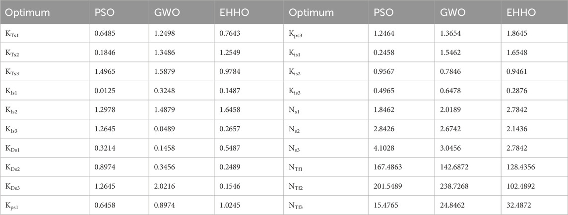
Table 2. Different parameters optimized with different algorithms.

6.3.1 GWO based controller

The performance of GWO based controller for SPV, WTG, BESS, DEG, load deviation and frequency deviation is shown and discussed in the following figures, the output power of SPV and WTG are 0.25 p. u and 0.36 p. u respectively. Also, the BESS and DEG response are shown in the figure. The GWO based controller has attained almost less load deviation compare to PSO. The GWO based controller for frequency deviation performance has achieved almost zero value with less deviation.

6.3.2 EHHO based proposed controller

The performance of EHHO based proposed controller compare with PSO and GWO for SPV, WTG, BESS, DEG, load deviation and frequency deviation of each microgrid area shows that the performance of proposed controller is achieving better results. The performance of the above controllers with respect to each microgrid area in comparison with PSO and GWO is shown in the following figures.

6.3.2.1 Microgrid Area-1

The performance of Microgrid area-1 under comparison of different optimization method is shown in the following figures. Figure 9A shows the output power of DEG and Figure 9B shows the output power of BESS Similarly, Figure 9C shows the frequency deviation of area-1 in Hz, also, and Figure 10D shows the total output power of area-1 in pu. From the figure it can be stated that the performance of EHHO shows better results compare to other optimization techniques in area-1.

Figure 9

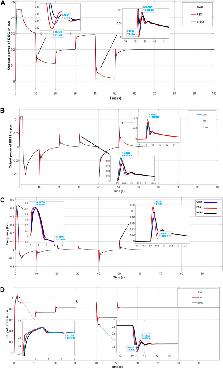
Figure 9. (A) Output power of DEG in pu, (B) Output power of BESS in pu, (C) Frequency deviation of area-1 in Hz, (D) The total output power of area-1 in pu.

Figure 10

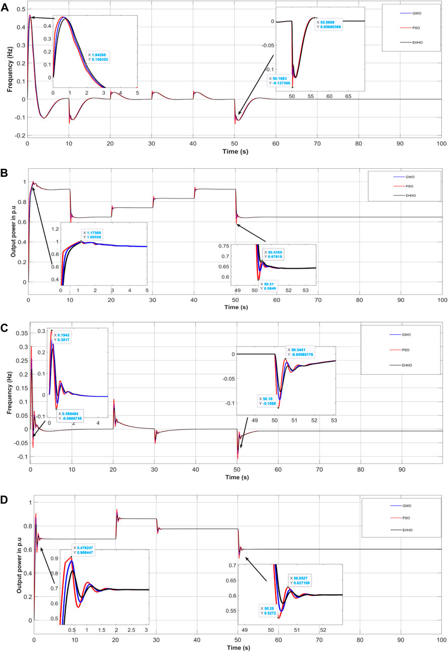
Figure 10. (A) Frequency deviation of area-2 in Hz, (B) The total output power of area-2 in pu, (C) shows the frequency deviation of area-3 in Hz, (D) Total output power of area-3 in pu.

6.3.2.2 Microgrid area 2 and area 3

Similar to area-1, the performance of Microgrid area-2 and area-3 under comparison of different optimization technique is shown in the following figures. Figure 10 (a) shows the frequency deviation of area-2 in Hz, also, and Figure 10B shows the total output power of area-2 in pu. From the figure it can be stated that the performance of EHHO shows better results compare to other optimization techniques in area-2. Likewise, Figure 10C shows the frequency deviation of area-3 in Hz, also, and Figure 10D shows the total output power of area-3 in pu. The output power and frequency deviation compare to area-1 shows better results in area-2 and area-3.

From the above figures, the proposed controller has attained better results compare to PSO and GWO. The SPV and WTG output for each area are not shown in the comparison due to stand alone configurations. As shown in the figure the response of the DEG and BESS tries to compensate the varying load and produce the corresponding output as per requirement of the system. The response of each area show better steady state with less variations under EHHO optimization schemes. Also, the frequency and output power of each area shown in the figure represents each response of area-1, -2 and -3. It can be seen that the proposed controller shows better results under different loads. The proposed controller is accurately minimize the load frequency deviation, i.e., the value of proposed controller has been almost converged to zero with less steady state error when compared to other methods such PSO and GWO. Therefore, the proposed controller has outperformed than existing techniques such as PSO and GWO.

6.4 Tie line values

The tie line of a transmission system is defined as the connecting point or parts of different transmission line or different sub-systems, here in microgrid system a tie line represents the connecting points of two or more area or branch for exchanging power for the whole microgrid system. the performance of each three Microgrid area under comparison of different optimization technique is discussed and shown in the previous subsections. However, comparison of each optimization technique in the tie line between each microgrid area is discussed in this section and the following figure shows tie line power and frequency. Figure 11 shows the tie line output power of (a) area-1 and area-2 (b) area-2 and area-3 and (c) area-1 and area-3. From the figure it can be stated that the performance of EHHO shows better results compare to other optimization techniques in area-3. Figure 11D shows tie line power deviation of different area under EHHO. Moreover, Figure 12 shows convergence plot comparison of PSO, GWO and EHHO optimization technique. The convergence curve shows that the fitness function for EHHO is low compared to other optimization technique and also converge faster. Also, Table 3 shows the parameters of each area of the microgrid system.

Figure 11

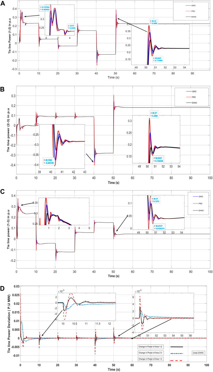
Figure 11. Tie line power of (A) area-1 and area-2, (B) area-2 and area-3, (C) area-1 and area-3, and (D) Tie line Power deviation of different area under EHHO.

Figure 12

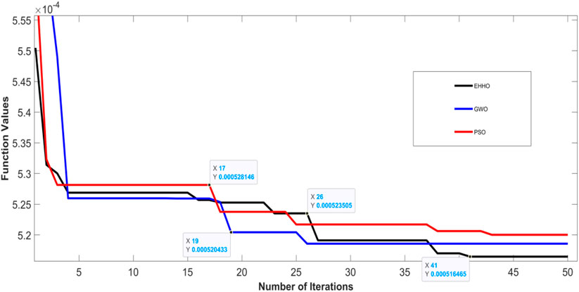
Figure 12. Comparison of convergence plot under PSO, GWO and EHHO optimization technique.

Table 3

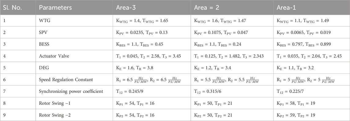
Table 3. Parameter values of each of the microgrid area-1, area-2 and area- 3.

7 Implementation of proposed controllers

7.1 3DOF-FOPIDN control structure

The PID controller is widely recognized as the foundational and primitive control technique that the field of control has ever developed. However, it has been observed that this controller may not perform well when the system is exposed to parameter changes, uneven disturbances, or non-linearities. To address these complications, the FO based-PID controller has been integrated with the concept of higher DOF. This integration provides additional features for tuning the controller and enhances its operating capabilities (Yousri et al., 2020).

To incorporate extra inertia and other important control, a fractional order controller (specifically, the double-stage FOPID (1 + PI) controller) has been employed. The proportional derivative (PD) component of the controller delivers the extra inertia and damping, while the integral (I) component offers additional regulator to the system. As a result, the controller derivative portion enhances the transient responses and improves the response of steady-state by minimizing the error (Khokhar et al., 2021).

A 3DOF (3 Degree of Freedom) controller consists of three independent feedback loops where three inputs, R(s), Y(s), and D(s), are obtained from each of the loops. The 3DOF structure is combined with a FOPIDN (Fractional Order Proportional Integral Derivative with Notch) controller to form a 3DOF-FOPIDN controller as shown in Figure 13. This new controller has an extra independent loop, which helps in achieving a better response compared to a 2DOF-FOPIDN controller.

Figure 13

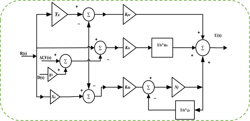
Figure 13. 3DOF-FOPIDN structure.

The fractional calculus involves using differentiation and integration with fractional-order or complex-order. Fractional derivatives have an advantage in that they can inherit the characteristics of the processes being modeled. The fractional-order PID controller (FO-PID) is a transfer function written as in Eq. 17.

$Controllerresponse\left(y\right)=D_a\Delta F+{KS}^{-\lambda }\Delta F+M_a{S}^{\mu }\Delta F\left(0<\lambda \le 1,0<\mu \le 0\right)(17)$

with gain constants, including a proportional part, D_a, an integral part, K, and a derivative part, Ma, with two fractional operators, λ and µ. The actuating signal of the 3DOF-FOPIDN controller is described by an equation, which takes into account the three inputs from the independent loops. The transfer functions of the FOPIDN controller is shown below.

$U\left(S\right)=\left\{y_x{k}_{px}+\frac{k_{ix}}{S^{\eta }}+x_x{k}_{dx}{s}^{\xi }\left(\frac{N_f}{{N_f+S}^{\xi }}\right)\right\}R\left(S\right)=\left\{-k_{px}+\frac{k_{ix}}{S^{\eta }}-k_{dx}{s}^{\xi }\left(\frac{N_f}{{N_f+S}^{\xi }}\right)\right\}Y\left(S\right)=\left\{{-g}_x{k}_{px}-\frac{k_{ix}}{S^{\eta }}{-g}_x{k}_{dx}{s}^{\xi }\left(\frac{N_f}{{N_f+S}^{\xi }}\right)\right\}D\left(S\right)(18)$

7.2 3DOF-TIDN control structure

In control systems, the degree of freedom (DOF) refers to the number of independent adjustments that can be made to the closed-loop transfer functions. By utilizing a 3DOF controller, closed-loop stability and dynamic response of the system can be improved while minimizing the effect of disturbances. The proposed 3DOF-TIDN controller is illustrated in Figure 14 which includes input reference R(S), system disturbance D(s), 3DOF output Y(s), and system output U(S). This controller is designed to enhance the dynamic response of the system by reducing the number of oscillations, minimizing deviation of frequency and tripping of power, and maintaining system stability. It is also intended to improve the damping ratio of the system in response to sudden loading changes (Ahmed et al., 2022). The output of the controller in a closed-loop configuration is mathematically expressed in an equation.

$Y\left(s\right)=\left[\frac{G_{CO}\left(s\right)G_P\left(s\right)}{1+G_{CO}\left(s\right)G_P\left(s\right)}{G}_{RC}\left(s\right)\right]R\left(s\right)+\left[\frac{G_P\left(s\right)-G_{CO}\left(s\right)G_P\left(s\right)G_{FFC}\left(S\right)}{1+G_{CO}\left(s\right)G_P\left(s\right)}\right]D\left(s\right)(19)$

Figure 14

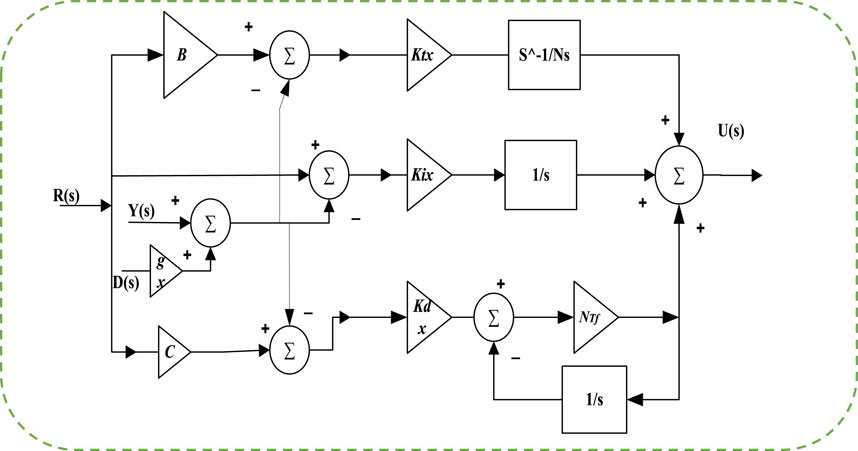
Figure 14. 3DOF-TIDN structure.

The GCO(s) is designed to limit certain parameters in the control system, such as tilt, integral, derivative gain (K_Ts, K_Is, K_Ds), tilt parameter (Ns), and low-pass filter (N_Tf). The proportional (B) and derivative (C) set point weights for R(s) are also represented by the GCO(s), while the gain parameter of the GFFC Controller is represented by G_x. To determine the optimal gain values for the controllers as well as parameters, an optimization algorithm is utilized, specifically the Enhanced Harris Hawks optimization algorithm, which minimizes the ITAE (Integral absolute error, Time, and Absolute Error), while adhering to certain constraints. These constraints include minimum and maximum bounds of 0 and 2 for the controller, 0 to 200 for the filters, and 2 to 3 for N.

$\left.\begin{array}{c}{K}_{Ts}^{\mathit{Min}}\le K_{Ts}\le K_{Ts}^{\mathit{Max}},K_{Is}^{\mathit{Min}}\le K_{Is}\le K_{Is}^{\mathit{Max}},K_{Ds}^{\mathit{Min}}\le K_{Ds}\le K_{Ds}^{\mathit{Max}}\\ N_{Tf}^{\mathit{Min}}\le N_{Tf}\le N_{Tf}^{\mathit{Max}},N_s^{\mathit{Min}}\le N_s\le N_s^{\mathit{Max}},{c^{\mathit{min}}}^{\mathit{Max}}\\ b^{{\mathit{min}}^{{\mathit{Max}}_{ff}^{{{\mathit{min}}_{ff}}_{ff}^{\mathit{Max}}}}\left.\right\}}\end{array}\right\}(20)$

When choosing between the 3DOF FOPIDN and 3DOF TIDN controllers for controlling three-degree-of-freedom mechanical systems, several differences should be considered. Firstly, the FOPIDN controller employs fractional calculus in its control approach, whereas the TIDN controller uses integer calculus. While the FOPIDN controller offers greater flexibility in adjusting control parameters, the TIDN controller may be simpler to implement. In terms of precision, the FOPIDN controller is generally regarded as more accurate than the TIDN controller due to its ability to utilize fractional calculus for control. Additionally, the FOPIDN controller is more robust, allowing it to effectively handle changes in the system or external disturbances. However, its implementation may be more complex than the TIDN controller, which relies on integer calculus and does not use notch filters (Guha et al., 2020).

Ultimately, the performance of each controller will depend on the specific application and the mechanical system being controlled. In some situations, the TIDN controller may be sufficient, while in others, the FOPIDN controller may be required for optimal performance. Therefore, the selection between the two controllers will depend on the specific requirements of the application and the mechanical system being controlled. Analysis of the controller in area-1, area-2 and area-3 are shown in the following figures.

Based on the analysis, the obtained results from Figures 15A–D demonstrate that the 3DOF-DOPIDN controller proposed in the study exhibits superior dynamic responses compared to other controllers. It effectively reduces oscillation and settling time in each area. Additionally, the controller helps to maintain the generated incremental power in the area. As there is no additional load demand, the total generated power in both areas remains at 0.04 p. u.MW. It also provides further insight into the controller’s performance by showing the power generation by various sources in area-2, which amounts to 2.5 p. u.MW peak in total.

Figure 15

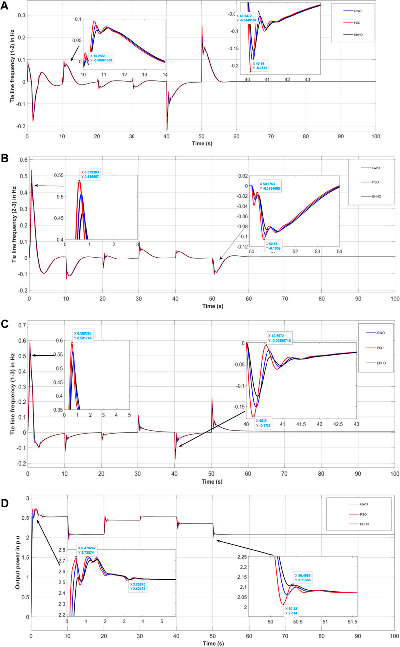
Figure 15. Tie line frequency deviation of (A) area-1 and area-2, (B) area-2 and area-3, (C) area-1 and area-3, and (D) Change in power of area-2.

Table 4 lists the gain values obtained for all three controllers studied in this section.

Table 4

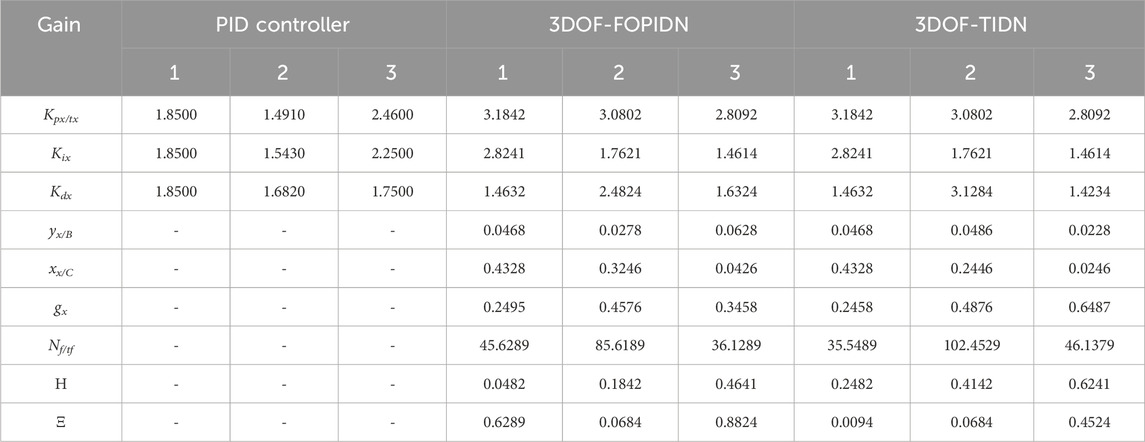
Table 4. Gain/weights/FO of controllers.

8 Stability analysis and robustness analysis

8.1 Stability analysis

To evaluate the stability of the system, an eigenvalue analysis is conducted with and without various secondary controllers while violating the contract. The eigenvalue plot is displayed in Figure 16 and listed in Table 5. The damping factor of the system is an indicator of how quickly the system is damped. The damping factors for the system are also provided in Table 5. The study examines several secondary controllers, including PID, 3DOF-TIDN, and 3DOF-FOPIDN.

Figure 16

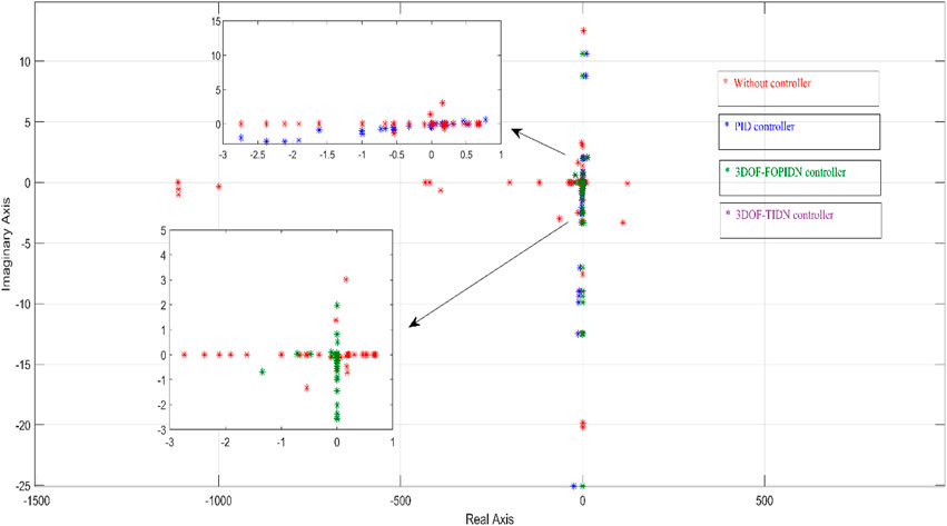
Figure 16. Comparison of Eigen value plot for proposed controllers.

Table 5

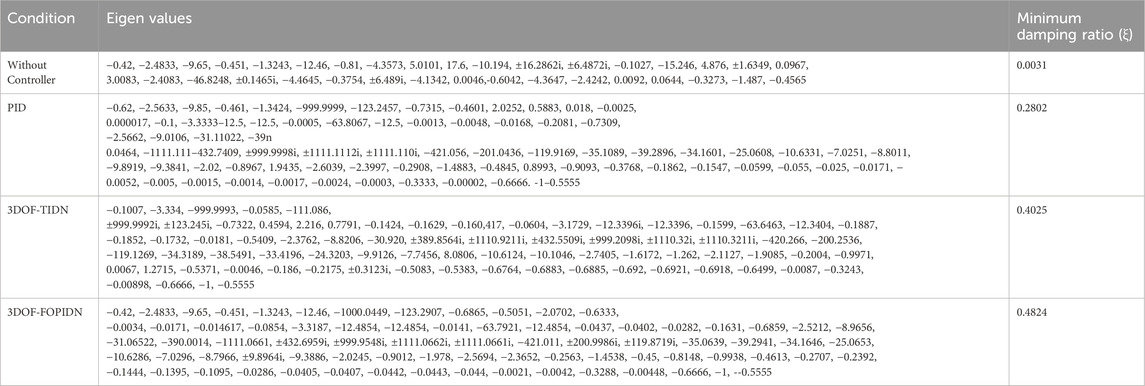
Table 5. Eigen Values of different controllers.

Upon analyzing the obtained eigenvalues, it was observed that the uncontrolled system had some eigenvalues in the right half of the s-plane, indicating instability. For the PID controllers, some of the eigenvalues were zero along with negative real parts, indicating marginal stability. However, it was observed from Figure 16 that the PID controllers resulted in initial system oscillations, but the system reached its steady-state value after some time. On the other hand, for the 3DOF-TIDN and 3DOF-FOPIDN controllers, all eigenvalues had negative real parts, indicating system stability. The damping ratio of the 3DOF-TIDN controller was found to be higher than others, indicating that the oscillation of the system may sustain for a smaller duration with this controller. Based on this analysis, it can be concluded that the 3DOF-FOPIDN controller provides more stable performance compared to the other controllers considered in the study.

8.2 Robustness analysis

Robustness analysis is a method used to evaluate the ability of a system, process, or product to maintain its performance even in the presence of uncertainties or changes in its operating conditions or environment. This analysis involves subjecting the system to different scenarios or inputs and analyzing its response to assess its performance. The objective of robustness analysis is to determine the system’s resilience and adaptability to various conditions and to identify the sources of variability and uncertainty that affect its performance.

The given passage describes a sensitivity analysis conducted to assess the robustness of a proposed 3DOF-FOPIDN controller by considering various scenarios and uncertainties. The analysis involves varying the parameters value in the system, such as varying the output of Wind, changing the system loading from the nominal scenario, and disconnecting one of the microgrid area. The results of the analysis are presented in Table 6, which shows the gains as well as other parameters under different scenarios. The system dynamics are then compared with the corresponding gain values of the 3DOF-FOPIDN controller equivalent to different conditions and their responses under nominal conditions.

Table 6

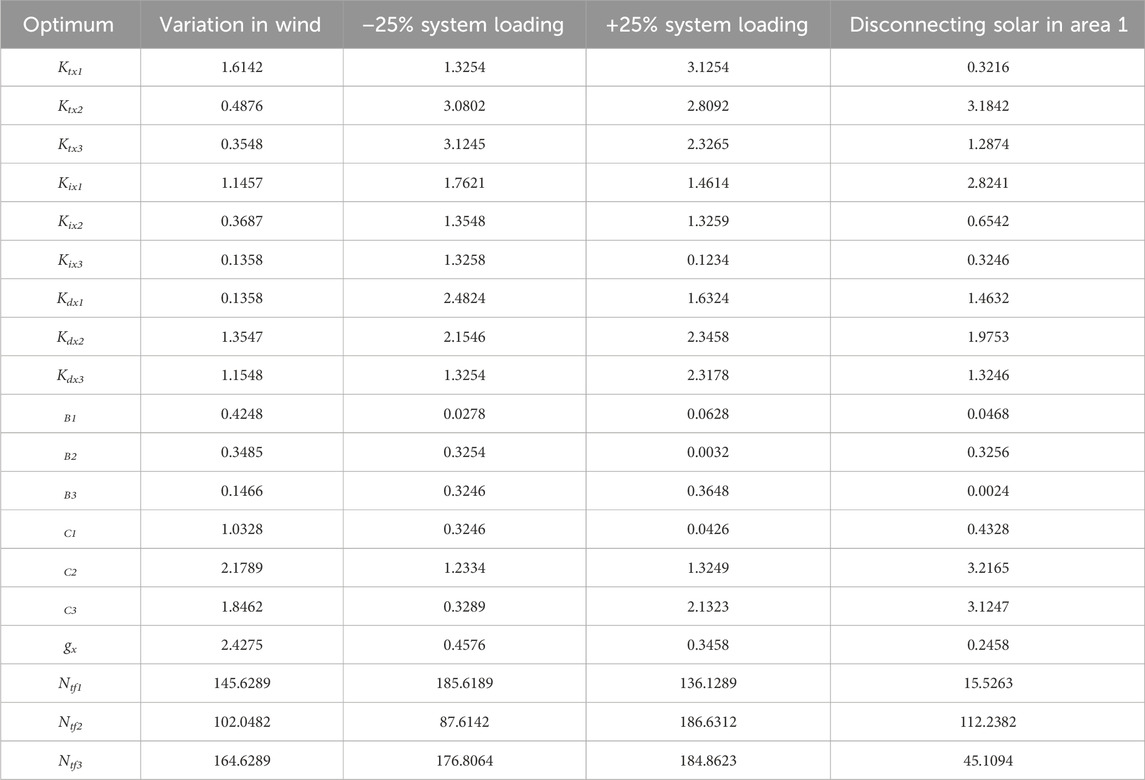
Table 6. Optimum values of 3DOF-FOPIDN controllers at different system conditions and system parameters.

Table 6 presents the ideal gains and other constraints for the 3DOF-FOPIDN controller based on the results of the sensitivity analysis. To compare the system dynamics, the gain values of the 3DOF-FOPIDN controller obtained under nominal conditions are used to generate responses for different scenarios. These responses are then compared to those obtained under changed conditions, as shown in Figures 17A, B. Overall, the sensitivity analysis involves six dynamic responses to evaluate the robustness of the 3DOF-FOPIDN controller.

Figure 17

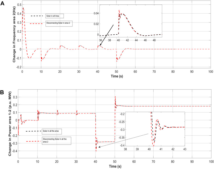
Figure 17. (A) Robustness frequency without solar in area-2, (B) Robustness Power without solar in area-2.

The system encountered a variation in its output, which increased from 0.006 p. u.MW to 0.012 p. u.MW. The gains as well as other constraints of the anticipated 3DOF-FOPIDN controller, taking into account various uncertainties, are listed in Table 6. To assess the controller’s robustness, its performance under the changed conditions is compared to its response under nominal conditions, using the gain values obtained from both scenarios. The resulting dynamic responses are presented in the below Figures.

8.2.1 Varying load of the system

In this particular case, the system’s loading was intentionally increased by 25% from its nominal value of 50% to examine the robustness of the controller’s gain values obtained under nominal conditions. Table 6 lists the gains as well as other constraints of the anticipated 3DOF-FOPIDN controller for various loading conditions. To assess the controller’s robustness, its performance under the changed conditions is compared to its response under nominal conditions, using the gain values obtained from both scenarios. The resulting dynamic results are shown in Figures 18A–C.

Figure 18

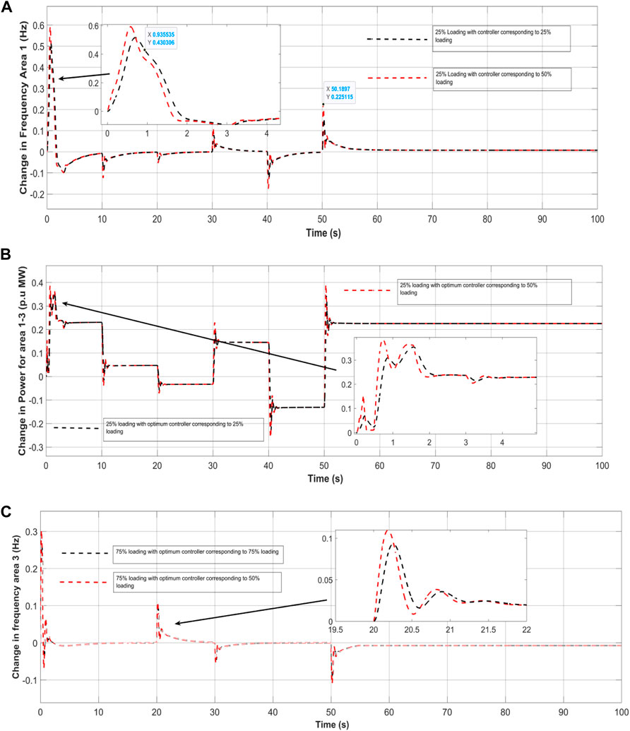
Figure 18. (A),Robustness under different loading frequency area-1, (B) Robustness under different loading power area 1–3. (C) Robustness under different loading (75% and 50%) frequency area-3.

8.2.2 Varying wind in area-2

To evaluate the robustness of the proposed controller’s gain values obtained at the nominal condition, the wind turbine in area-2 were disconnected, while considering the system loading and power generation in all areas. The gains as well as constraints of the anticipated 3DOF-FOPIDN controller in this scenario are shown in Table 6. To validate the controller’s robustness, the system responses were compared using the gain values of the 3DOF-FOPIDN controller equivalent to changed conditions with the results obtained under nominal conditions. The total power generation microgrid in area-2 is depicted in Figures 19A, B.

Figure 19

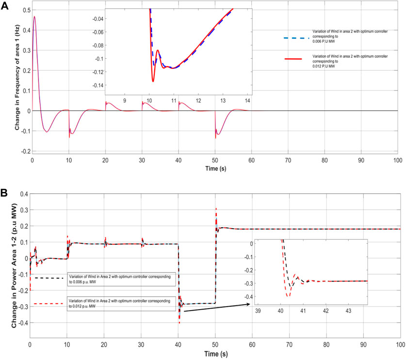
Figure 19. (A) Variation in wind turbine output considering frequency of area-1, (B) Variation in wind output considering change in power of area-1 and area-2.

9 Conclusion/analysis

This paper introduces a novel approach to controlling frequency deviation in a multi-microgrid system with RES and DEG, taking into consideration the power supply of a WTP with various pumping and power stations. The proposed system incorporates different energy sources such as DEG, SPV, WTG, and BESS as power sources for each area of the microgrid system. To enhance the performance of the PID controller, the tuning parameters are optimally selected using the EHHO method. The performance of the proposed controller is then compared to existing techniques, such as PSO and GWO, using MATLAB software. Load demand and frequency are used to analyze and evaluate the performance of the proposed controller. The results show that the proposed EHHO-based PID controller effectively regulates the load frequency deviation in a RES-based multi-microgrid system. In comparison to PSO and GWO, the proposed controller outperforms these existing techniques, demonstrating better performance for controlling load frequency deviation.

Furthermore, the paper discussed about the design of an ideal control method using a 3DOF-FOPIDN controller based on PSO algorithm to improve system dynamic performance. The outcome indicates that the 3DOF-FOPIDN controller shows better results compare to other secondary controllers viz. 3DOF-TIDN in reducing oscillations, settling time, and tie line deviation of power. Finally, the study shows that the 3DOF-FOPIDN controller is robust enough to handle uncertain oscillations as well as changes, such as the removal of Solar, discrepancy of the wind speed, and changing the inertia of the system, without needing repeated resetting of controller parameters.

Data availability statement

The original contributions presented in the study are included in the article/Supplementary material, further inquiries can be directed to the corresponding authors.

Author contributions

CR: Writing–original draft, Writing–review and editing. Subir Datta: Writing–original draft, Writing–review and editing. Nidul Sinha: Writing–original draft, Writing–review and editing. KS: Writing–original draft, Writing–review and editing. Subhasish DeB: Writing–original draft, Writing–review and editing. UC: Writing–original draft, Writing–review and editing. TU: Writing–original draft, Writing–review and editing.

Funding

The author(s) declare that no financial support was received for the research, authorship, and/or publication of this article.

Conflict of interest

The authors declare that the research was conducted in the absence of any commercial or financial relationships that could be construed as a potential conflict of interest.

Publisher’s note

All claims expressed in this article are solely those of the authors and do not necessarily represent those of their affiliated organizations, or those of the publisher, the editors and the reviewers. Any product that may be evaluated in this article, or claim that may be made by its manufacturer, is not guaranteed or endorsed by the publisher.

References

Abdolrasol, G. M., Hannan, M. A., Hussain, S. M. S., Ustun, T. S., Sarker, M. R., and Ker, P. J. (2021). Energy management scheduling for microgrids in the virtual power plant system using artificial neural networks. Energies 14, 6507. doi:10.3390/en14206507

CrossRef Full Text | Google Scholar

Adefarati, T., Bansal, R. C., and Justo, J. J. (2017). Techno-economic analysis of a PV-wind-battery-diesel standalone power system in a remote area. J. Eng. 2017 (13), 740–744. doi:10.1049/joe.2017.0429

CrossRef Full Text | Google Scholar

Ahmed, M., Magdy, G., Khamies, M., and Kamel, S. (2022). Modified TID controller for load frequency control of a two-area interconnected diverse-unit power system. Int. J. Elect. Power Energy Syst. 135, 107528. doi:10.1016/j.ijepes.2021.107528

CrossRef Full Text | Google Scholar

Babazadeh, M., and Karimi, H. (2013). A robust two-degree-of-freedom control strategy for an islanded microgrid. IEEE Trans. power Deliv. 28 (3), 1339–1347. doi:10.1109/tpwrd.2013.2254138

CrossRef Full Text | Google Scholar

Baghaee, H. R., Mirsalim, M., Gharehpetian, G. B., and Talebi, H. A. (2017). Three-phase AC/DC power-flow for balanced/unbalanced microgrids including wind/solar, droop-controlled and electronically-coupled distributed energy resources using radial basis function neural networks. IET Power Electron. 10 (3), 313–328. doi:10.1049/iet-pel.2016.0010

CrossRef Full Text | Google Scholar

Barik, A. K., Das, D. C., Latif, A., Hussain, S. M. S., and Ustun, T. S. (2021). Optimal voltage–frequency regulation in distributed sustainable energy-based hybrid microgrids with integrated resource planning. Energies 14, 2735. doi:10.3390/en14102735

CrossRef Full Text | Google Scholar

Chakraborty, M. R., Dawn, S., Saha, P. K., Basu, J. B., and Ustun, T. S. (2022). A comparative review on energy storage systems and their application in deregulated systems. Batteries 8, 124. doi:10.3390/batteries8090124

CrossRef Full Text | Google Scholar

Chauhan, A., Upadhyay, S., Khan, M. T., Hussain, S. M. S., and Ustun, T. S. (2021). Performance investigation of a solar photovoltaic/diesel generator based hybrid system with cycle charging strategy using BBO algorithm. Sustainability 13, 8048. doi:10.3390/su13148048

CrossRef Full Text | Google Scholar

Dey, P. P., Das, D. C., Latif, A., Hussain, S. M. S., and Ustun, T. S. (2020). Active power management of virtual power plant under penetration of central receiver solar thermal-wind using butterfly optimization technique. Sustainability 12, 6979. doi:10.3390/su12176979

CrossRef Full Text | Google Scholar

Gheisarnejad, M., and Khooban, M. H. (2019). Secondary load frequency control for multi-microgrids: HiL real-time simulation. Soft Comput. 23 (14), 5785–5798. doi:10.1007/s00500-018-3243-5

CrossRef Full Text | Google Scholar

Guha, D., Roy, P. K., and Banerjee, S. (2020). Equilibrium optimizer-tuned cascade fractional-order 3DOF-PID controller in load frequency control of power system having renewable energy resource integrated. Int. Trans. Elect. Energy Syst. 31, 1–25. doi:10.1002/2050-7038.12702

CrossRef Full Text | Google Scholar

He, J., Li, Y., Liang, B., and Wang, C. (2017). Inverse power factor droop control for decentralized power sharing in series-connected micro-converters based islanding microgrids. IEEE Trans. Ind. Electron. 64 (9), 7444–7454. doi:10.1109/tie.2017.2674588

CrossRef Full Text | Google Scholar

Hossain, M. A., Pota, H. R., Hossain, M. J., and Blaabjerg, F. (2019). Evolution of microgrids with converter-interfaced generations: challenges and opportunities. Int. J. Electr. Power and Energy Syst. 109, 160–186. doi:10.1016/j.ijepes.2019.01.038

CrossRef Full Text | Google Scholar

Karimi, Y., Oraee, H., and Guerrero, J. M. (2016). Decentralized method for load sharing and power management in a hybrid single/three-phase-islanded microgrid consisting of hybrid source PV/battery units. IEEE Trans. Power Electron. 32 (8), 6135–6144. doi:10.1109/tpel.2016.2620258

CrossRef Full Text | Google Scholar

Khokhar, B., Dahiya, S., and Parmar, K. P. S. (2021). A novel hybrid fuzzy PD- TID controller for load frequency control of a standalone microgrid. Arab. J. Sci. Eng. 46, 1053–1065. doi:10.1007/s13369-020-04761-7

CrossRef Full Text | Google Scholar

Kikusato, H., Ustun, T. S., Suzuki, M., Sugahara, S., Hashimoto, J., Otani, K., et al. (2022). Flywheel energy storage system based microgrid controller design and PHIL testing. Energy Rep. 8 (10), 470–475. doi:10.1016/j.egyr.2022.05.221

CrossRef Full Text | Google Scholar

Latif, A., Paul, M., Das, D. C., Hussain, S. M. S., and Ustun, T. S. (2020). Price based demand response for optimal frequency stabilization in ORC solar thermal based isolated hybrid microgrid under salp Swarm technique. Electronics 9, 2209. doi:10.3390/electronics9122209

CrossRef Full Text | Google Scholar

Li, X., Song, Y. J., and Han, S. B. (2008). Frequency control in MicroGrid power system combined with electrolyzer system and fuzzy PI controller. J. Power Sources 180 (1), 468–475. doi:10.1016/j.jpowsour.2008.01.092

CrossRef Full Text | Google Scholar

Mishra, S., Prusty, R. C., and Panda, S. (2020). Design and analysis of 2dof-PID controller for frequency regulation of multi-microgrid using hybrid dragonfly and pattern search algorithm. J. Control, Automation Electr. Syst. 31, 813–827. doi:10.1007/s40313-019-00562-y

CrossRef Full Text | Google Scholar

Nayak, S. R., Khadanga, R. K., Panda, S., Sahu, P. R., Padhy, S., and Ustun, T. S. (2023). Participation of renewable energy sources in the frequency regulation issues of a five-area hybrid power system utilizing a sine cosine-adopted african vulture optimization algorithm. Energies 16, 926. doi:10.3390/en16020926

CrossRef Full Text | Google Scholar

Obaid, Z. A., Cipcigan, L. M., Abrahim, L., and Muhssin, M. T. (2019). Frequency control of future power systems: reviewing and evaluating challenges and new control methods. J. Mod. Power Syst. Clean Energy 7 (1), 9–25. doi:10.1007/s40565-018-0441-1

CrossRef Full Text | Google Scholar

Rohmingtluanga, C., Datta, S., Sinha, N., and Ustun, T. S. (2023). SCADA based intake monitoring for improving energy management plan: case study. Energy Rep. 9 (1), 402–410. doi:10.1016/j.egyr.2022.11.037

CrossRef Full Text | Google Scholar

Rohmingtluanga, C., Datta, S., Sinha, N., Ustun, T. S., and Kalam, A. (2022). ANFIS-based droop control of an AC microgrid system: considering intake of water treatment plant. Energies 15, 7442. doi:10.3390/en15197442

CrossRef Full Text | Google Scholar

Sreedharan, P., Farbes, J., Cutter, E., Woo, C., and Wang, J. (2016). Microgrid and renewable generation integration: university of California, san diego. Appl. Energy 169, 709–720. doi:10.1016/j.apenergy.2016.02.053

CrossRef Full Text | Google Scholar

Tchobanoglus, G., Burton, F., and Stensel, H. D. (2003). Wastewater engineering: treatment and reuse. Am. Water Works Assoc. J. 95 (5), 201.

Google Scholar

Ulutas, A., Altas, I. H., Onen, A., and Ustun, T. S. (2020). Neuro-Fuzzy-based model predictive energy management for grid connected microgrids. Electronics 9, 900. doi:10.3390/electronics9060900

CrossRef Full Text | Google Scholar

Vafamand, N., Khooban, M. H., Dragičević, T., Boudjadar, J., and Asemani, M. H. (2019). Time-delayed stabilizing secondary load frequency control of shipboard microgrids. IEEE Syst. J. 13 (3), 3233–3241. doi:10.1109/jsyst.2019.2892528

CrossRef Full Text | Google Scholar

Wentzel, J., Ustun, T. S., Ozansoy, C., and Zayegh, A. (2012). “Investigation of micro-grid behavior while operating under various network conditions,” in 2012 International Conference on Smart Grid (SGE), Oshawa, ON, Canada, 1–5. doi:10.1109/SGE.2012.6463973

CrossRef Full Text | Google Scholar

Yammani, C., and Maheswarapu, S. (2019). Load frequency control of multi-microgrid system considering renewable energy sources using grey wolf optimization. Smart Sci. 7 (3), 198–217. doi:10.1080/23080477.2019.1630057

CrossRef Full Text | Google Scholar

Yousri, D., Babu, T. S., and Fathy, A. (2020). Recent methodology based Harris Hawks optimizer for designing load frequency control incorporated in multi-interconnected renewable energy plants. Sustain. Energy Grids Netw. 22, 100352. doi:10.1016/j.segan.2020.100352

CrossRef Full Text | Google Scholar

Zhang, C., Xu, Y., Dong, Z. Y., and Wong, K. P. (2017). Robust coordination of distributed generation and price-based demand response in microgrids. IEEE Trans. Smart Grid 9 (5), 4236–4247. doi:10.1109/tsg.2017.2653198

CrossRef Full Text | Google Scholar

Zhang, Z., Kusiak, A., Zeng, Y., and Wei, X. (2016). Modeling and optimization of a wastewater pumping system with data-mining methods. Appl. Energy 164, 303–311. doi:10.1016/j.apenergy.2015.11.061

CrossRef Full Text | Google Scholar