Refinement of the daily precipitation simulated by the CMIP5 models over the north of the Northeast of Brazil

Introduction

The Intertropical Convergence Zone (ITCZ) is the main meteorological system in large scale responsible for the rainy season over the north of the Northeast of Brazil (NEB) (Hastenrath et al., 1984; Xie and Carton, 2004 and references therein). This system is a semi-permanent low-pressure band of clouds that circle the globe near the equator on the confluence region of the southeasterly and northeasterly trade winds from the Southern and Northern Hemispheres, respectively. Climatologically the ITCZ follows the seasonal march of the sun: the northernmost position occurs in July to September and the southernmost position is observed during December to February (Biasutti et al., 2003). As reported by Xie and Carton (2004) there is an apparent lag in the meridional excursion of the continental precipitation band. The possible causes are the heat reservoirs such as soil moisture and oceanic influences.

The rainy season over north of the NEB occurs due the meridional position of ITCZ closest to this region. The seasonality or persistence of warm waters over the Tropical South Atlantic favors the transport of the moisture into the interior of the NEB. In opposite, in periods in which the ITCZ is anomalously to the northward are expected drought conditions over the north of the NEB. As mentioned in Grodsky and Carton (2003) the anomalous displacement to the northward occurs in the presence of changes in inter-hemispheric Sea Surface Temperature (SST) gradient over the Atlantic Ocean. The development of the equatorial cold tongue in June persisting through September month maintains the ITCZ to the northward of the equator.

In general, the climate models show high degree skill in simulating the precipitation over the NEB region (Misra, 2004) in comparison with others regions of Brazil. Such characteristic is explained in part due the linear processes that dominate over the nonlinear processes in this region. The linear processes are influenced directly by the modifications in Hadley and Walker Cells in response to interannual variability in SST field over the Equatorial Eastern Pacific and the local impact of the South Tropical Atlantic Ocean. However, the nonlinear signal is influenced by SST variability that is found over others oceanic basins as the North Atlantic (Kayano and Andreoli, 2004) the North Pacific (Kayano and Andreoli, 2004; da Silva et al., 2011) and the Indian Ocean (Taschetto and Ambrizzi, 2012). The large SST anomalies over these oceanic basins seem to influence indirectly the linear impact and consequently the precipitation variability over the NEB. As mentioned in Silva et al. (2014) the precipitation field shows an inherent complexity determined by the global water cycle in association with the behavior of many factors such as moisture distribution over the continents, thermodynamics, and dynamical aspects, among others. This variable has an extreme relevance due the direct importance in many sectors of the society and environment. However, the spatial and temporal variability of the precipitation are not yet reproduced satisfactorily by the numerical models. This leads some questions that are addressed in present study:

(i) Are the CMIP5 models able to reproduce the main rainy season over the north of the NEB during the present climate?

(ii) What is the more adequate statistical downscaling approach to improve the model simulations during the present climate: the Artificial Neural Network (ANN) or the Multiple Linear Regression (MLR)?

(iii) Which one of these statistical models is more appropriate to project future scenarios of climate change based on CMIP5 runs?

It is worth mentioning that the scope of this paper is simple but efficient analyses relative to the performance of the ANN and MLR models to improve the General Circulation Models (GCMs) outputs. However, a brief discussion regarding the anomalous structure of the simulated ITCZ by these models is described to help in interpretation of the results. The statistical downscaling is used in this study as a refinement method to bridge the complex relationship between the large-scale and local atmospheric features for the present climate. The captured relationships are also designed to project regional climate change from direct outputs of the GCMs. The MLR have been introduced into meteorology and oceanography as a statistical model in a first stage in comparison with the ANN that is more recent at ends of 1990s approximately.

The ANN is able to learn and generalize the nonlinear relations between the predictor and predictand datasets. It also does not require a priori knowledge of the process. The disadvantage is that the relations learned are hidden in the structure not described in mathematical expression. The MLR captures the linear relations between these datasets that can be expressed in mathematical terms. The limitation of this model is the priori assumption about the consistency of this relationship.

The literature refers to the statistical downscaling through the ANN as an alternative to minimize the deficiencies of the GCMs (Gardner and Dorling, 1998). The technique allows the establishment of statistical links between the observed large-scale circulation and the precipitation or temperature fields by applying transfer functions to the GCMs outputs. Recently, Silva and Mendes (2013) elaborated a ANN model using as predictand variables the seasonal hindcasts of precipitation anomalies from the Climate Forecast System v2 (CFSv2) model and the observed dominant modes of anomalous SST over the South and North Atlantic to reproduce the precipitation during the rainy seasons over the south and north of the NEB region. The authors obtained fairly success in using the ANN approach as a complementary tool for the climate studies. However, there are few studies that explore the temporal downscaling by using the ANN method over the NEB region. The literature is focus mainly over the Amazon Basin (Mendes and Marengo, 2010; Mendes et al., 2014) and Southeast (Johnson et al., 2012) and South of Brazil (Ramírez et al., 2006).

The main objectives of the present study are twofold: to compare the performance of the temporal nonlinear (ANN) and linear (MLR) downscaling methods in predict the area-average observed daily precipitation during the rainy season over the north of the NEB for the present climate; and to examine the accuracy of the more adequate statistical method in project changes for the future climate over the same region. To investigate the future climate we use the CMIP5 model outputs forced by the Representative Concentration Pathways 8.5 (RCP8.5) scenario that is derived directly from the A2r scenario (Riahi et al., 2007). The choice for the RCP8.5 scenario is that in comparison with the others RCPs it corresponds to the pathway with the highest greenhouse gas emissions and concentrations leading to radiative forcing of 8.5 W.m⁻¹ at the end of the century (Moss et al., 2010). The assumptions are summarized in Riahi et al. (2011): high population and relatively slow income growth with modest rates of technological change and energy intensity improvements, leading in the long term to high energy demand and greenhouse gas emissions in absence of climate change policies.

Section Materials and Methods describe the design of the statistical simulations. Section Results for the present and future climate analyses and the Section Summary refers to the main results.

Materials and Methods

The region of study is the north of the NEB that is detached by the red box between 2 and 7°S; 40 and 45°W as displayed in Figure 1. The 41 years of observed daily precipitation data for the present climate of 1963–2003 period derived from the South America 24 Gridded Precipitation dataset – SA24 (Liebmann and Allured, 2005) is obtained over this region. For the same period, we used the historical simulations of precipitation derived from the Coupled Model Intercomparison Project phase 5-CMIP5/IPCC (http://cmip-pcmdi.llnl.gov/cmip5). The projections of changes in precipitation field for the future climate of the 2055–2095 periods are obtained from the CMIP5 models forced with the high emission scenario RCP8.5 (940 ppm) as shown in Table 1.

FIGURE 1

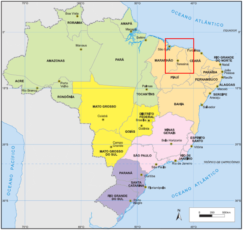
Figure 1. Location of the study region: North of the NEB delimited by the red box between 2 and 7°S; 40 and 45°W. The location is similar as in Silva and Mendes (2013). Adapted from http://mapas.ibge.gov.br.

TABLE 1

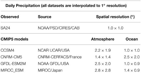
Table 1. Observed and CMIP5 models daily precipitation dataset.

For the observations the area-averaged daily precipitation is calculated over the study area during the rainy season from Feb–Mar–Apr (FMA) and for two previous lag months from Dec-Jan-Feb (DJF). The correlation between the observed daily precipitation during DJF and FMA is also calculated. Also, the differences between the normalized time series of the observed daily precipitation and the CMIP5 simulations during FMA season are shown. To explain such differences is calculated the anomalies of SST and precipitation over the Atlantic Ocean using as observations the ERSST version3b (Smith et al., 2008) and CAMS_OPI v0208 (Janowiak and Xie, 1999) datasets, respectively. All dataset are interpolated to a 1° lat-lon grid as in observations. Regarding the future climate period we also calculated the area-averaged daily precipitation during FMA season as derived from the CMIP5 runs.

The performance of the temporal downscaling through the ANN and MLR is compared with emphasis in ability to predict the tendency during present climate. Changes projected for the future climate derived directly from the grid box daily precipitation simulated by the CMIP5 models are compared with the changes simulated indirectly through the ANN. For the ANN and MLR methods the simulations are designed as in Table 2.

TABLE 2

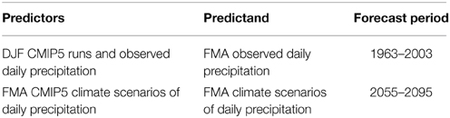
Table 2. Design of the statistical downscaling with the ANN model.

The ANN model is based in a learning technique in parallel. Through a sequence of predictors variables designed as input the network is trained to fit weights for those that can have contributed to the variability of predicted variables (target dataset). The learning technique has an advantages of generalization in which the input dataset should be divided in training (used to obtain the network weights), validation (used to obtain the accuracy of the model), and test (used to obtain the realistic estimative of the performance of the model). The network maps the predictors in a second set of output variables that are compared with the desired target and corrections are made until the model reaches the lowest possible error. In our study the skill model is analyzed through the Mean Squared Error (MSE), the linear correlation coefficient (corr) and the bias. The ANN has a capacity to identify approximate nonlinear relations between the predictor and predictand and their derivatives without a prior knowledge of a specific nonlinear function (Ramírez et al., 2006).

As in Silva and Mendes (2013) the Multilayer Perceptron architecture is used that is more adequate network for meteorological applications because the weather and the climate can repeat along the chronological time but never exactly in the same way (e.g., Cardoso and da Silva Dias, 2004). The Figures 2, 3 represent the topology of the ANN used in the present study for the present and future climate analyses, respectively. For both simulations the Multilayer Perceptron topology is interconnected in a feed-forward method. This method allows that the information of one hidden layer with the eight tangent sigmoid neurons be forward in direction of the input nodes to the output nodes.

FIGURE 2

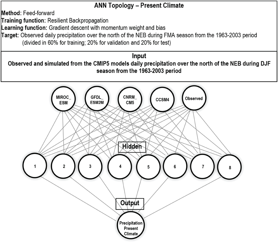
Figure 2. ANN topology used for the present climate simulations.

FIGURE 3

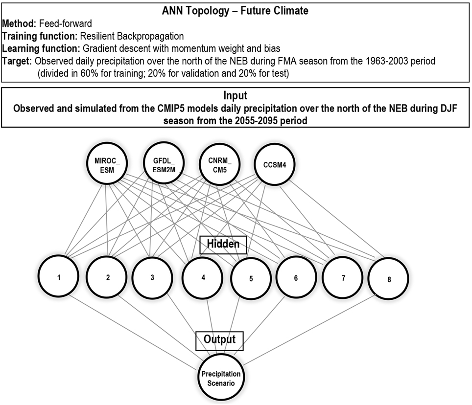
Figure 3. ANN topology used for the future climate simulations.

The resilient backpropagation is the training function with a gradient descent, and the momentum weight and bias is the learning function. The training function used allows eliminating the effect of the sigmoid transfer function in the hidden layer. The effect surges when the input is large that forces to their gradient must approach zero tending to very small magnitude values favoring low changes in the weights and biases. To estimate the accuracy and reduce the effect of over-fitting, the cross-validation is applied. For instance, the training dataset is divided in 60% for training; 20% for validation; and 20% for test.

In Figure 2 the target dataset is the observed daily precipitation during FMA season of 1963–2003 over the north of the NEB. The input is the daily precipitation during DJF season of the same period and region that are extracted from the observations and CMIP5 outputs. The result of the ANN model is the output relative to the daily precipitation simulated for the present climate during FMA season. In Figure 3 for the future climate analyses the target is the daily precipitation during FMA season of the 1963–2003 previously predicted through the ANN. The input dataset are the values of precipitation for the FMA season of the 2055–2095 periods and the output is simulation of the ANN model relative to the precipitation scenario for the FMA season.

The Equation (1) express the MLR model in which a output y (predictand) is dependent of a set of input (predictors) that are independent variables x₁, x₂, …, x_p (p > 1). The values α is the y-intercept, β_k(k = 1, 2, …, p) are the weights and ϵ is the forecast error.

$\begin{array}{cc}y=\alpha +{\displaystyle \sum _k{\beta }_k{x}_k+\in }& (1)\end{array}$

The idea in using the MLR is to adjust predictors that are a set of daily precipitation during DJF season over the north of the NEB derived from the CMIP5 models to a predictand, the observed daily precipitation during FMA season over the same area. This implies in identify the lagged influence of each CMIP5 model in capture the most part of the variability in precipitation over the study region.

For the ANN and MLR models the predictors and predictand variables are normalized in interval [0, 1] by min-max formula similar as Sajikumar and Thandaveswara (1999):

$\begin{array}{cc}v\prime \left(i\right)=\frac{v\left(i\right)-mi{n}_{i}v(i)}{ma{x}_{i}v\left(i\right)-mi{n}_{i}v(i)}& (2)\end{array}$

A posterior normalization in interval [−1,1] is assuming that

$\begin{array}{cc}v″=av\prime +b& (3)\end{array}$

So, when: v′ = 0, v″ = −1; when v′ = 1, v″ = 1 implying that −1 = b and 1 = a + b′ resulting in:

$\begin{array}{cc}v″=2v\prime -1& (4)\end{array}$

Results

Present Climate

The observed and simulated normalized time series of daily precipitation for FMA season are displayed in Figure 4. The observed anomalies in Figure 4A are calculated in relation to the mean of 8.13 mm.day⁻¹. The median value of 8.21 mm.day⁻¹ suggests that the extremes in normalized time series do not affect the mean value. The Figure 4B show high discrepancies between the CMIP5 outputs in modeling the present-day precipitation for FMA season. The MIROC_ESM model simulates the worst results overestimating the precipitation during the Feb–Mar months and underestimating in April. The GFDL_ESM2M model underestimates the daily precipitation amplitude along the time series and the CNRM_CM5 model shows a higher variability an extreme values. The differences between the models in modeling the large-scale precipitation patterns imply that is necessary to considerer the use of statistical techniques to improve the present simulation and future climate projections. In others, is relevant to apply the refinement methods in the GCMs outputs mainly in improving of their mean and variability.

FIGURE 4

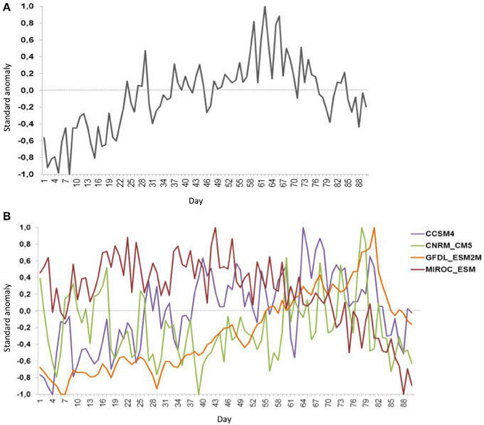
Figure 4. Observed (A) and simulated from the CMIP5 models (B) daily precipitation over the north of the NEB during FMA season from the 1963–2003 period.

The outputs from the CCSM4, GFDL_ESM2M, and MIROC_ESM models during DJF season are most correlated with the observed FMA season precipitation (Table 3). The correlations values are of 0.54, 0.66, and 0.66, respectively. However, only the CCSM4 model displays a slightly reasonable agreement in terms of variability in the normalized series. The considerable differences in the mean and the variability between the observed and modeled daily precipitation values justify the differences found in correlations observed in the Table 3.

TABLE 3

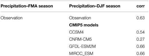
Table 3. Lagged correlation between the normalized daily precipitation time series derived from the CMIP5 models for the DJF season and observed for the FMA season during the 1963–2003 period.

In order to investigate these discrepancies we compare the simulated mean SST and precipitation from each model over the Equatorial Atlantic Ocean with the observed field (Figures 5A,B, 6A,B, respectively) that results in the anomalous fields (Figures 5C–J, 6C–J, respectively). The observed SST for the DJF season shows a warm pool in a region extending into the 5–8°S with values of 26–28°C and maximum magnitude on the eastern basin. The precipitation band is located over the equator region, between 5°S and 8°N onto which the trade winds converge from the North and South Hemispheres (Figures 5A, 6A, respectively). During FMA season the warm pool intensifies along the central basin and coast of the NEB and vicinity of the Equatorial Atlantic Ocean. As response an intensification of the precipitation along these regions is observed during FMA season with a notable maximum nucleus over the north of the NEB (Figures 5B, 6B, respectively).

FIGURE 5

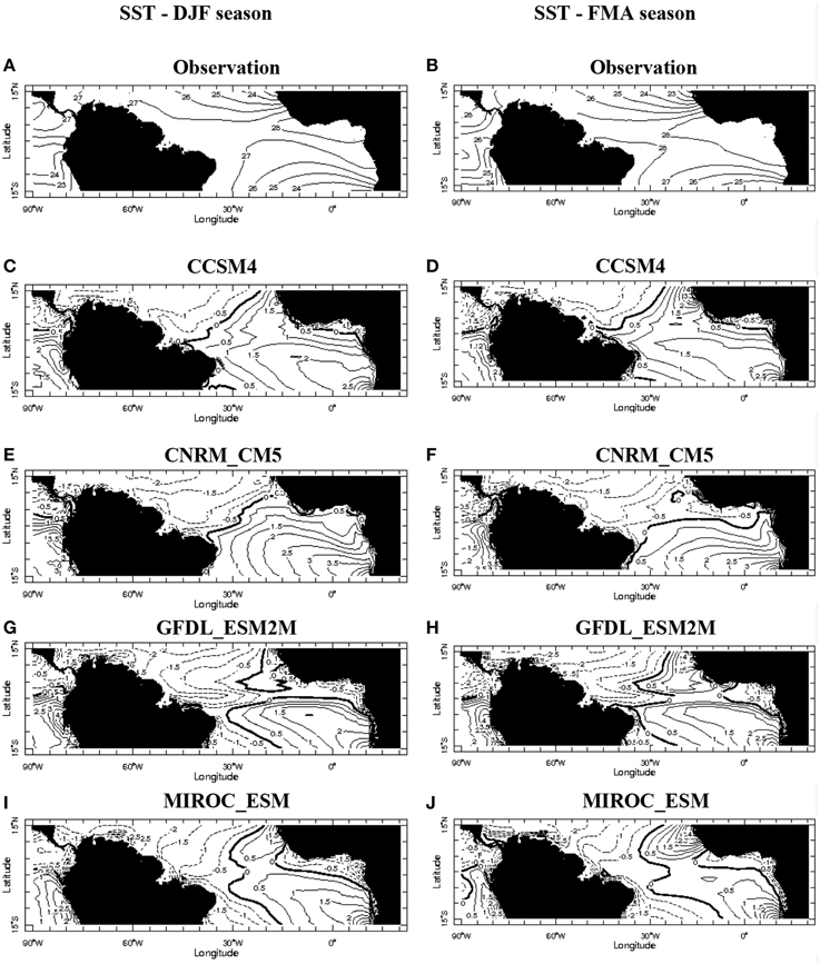
Figure 5. On the left panel the DJF mean SST during 1963–2003 period along the equator area for the observation (letter A) and the DJF anomalies for the CCSM4, CNRM_CM5, GFDL_ESM2M e MIROC_ESM models (letters C, E, G, and I respectively). On the right panel the same sequence as on the left panel except for FMA (the mean in B, and the anomalies in D, F, H, J). All data are interpolated to a lat-lon grid with 1°. The respective maps were constructed from the IRI/LDEO Climate Data Library.

FIGURE 6

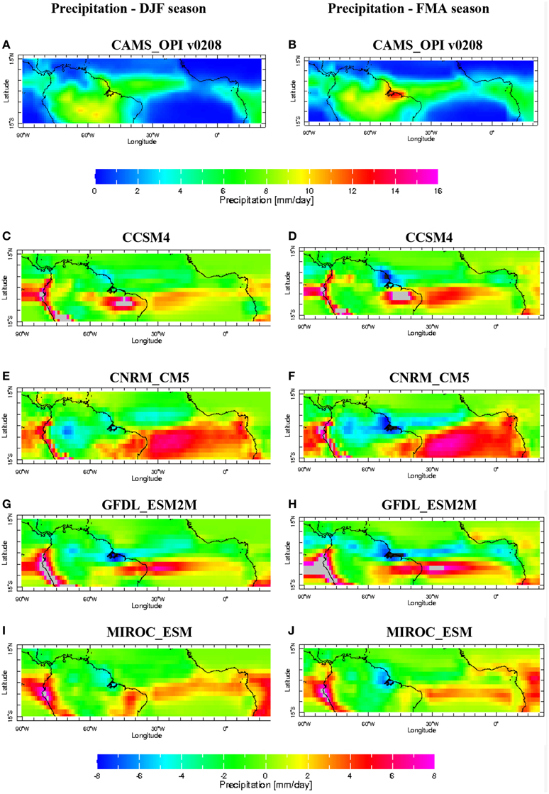
Figure 6. On the left panel the DJF mean precipitation during 1963–2003 period along the equator area for the observation (letter A) and the DJF anomalies for the CCSM4, CNRM_CM5, GFDL_ESM2M e MIROC_ESM models (letters C, E, G, and I, respectively). On the right panel the same sequence as on the left panel except for FMA (the mean in B, and the anomalies in D, F, H, J). All data are interpolated to a lat-lon grid with 1°. The respective maps were constructed from the IRI/LDEO Climate Data Library.

Siongco et al. (2014) analyzed 24 of the CMIP5 models and found significant deficiencies in reproduction of the ITCZ structure with either the west or the east Atlantic bias and no model matches the observed precipitation distribution. Our analysis for the DJF and FMA seasons shows that the CCSM4, CNRM_CM5, GFDL_ESM2M, and MIROC_ESM models have a cooling (warming) bias over the western (eastern) basin with anomalies below −0.5°C (above 0.5°C). The more intense values are found on the eastern Equatorial Atlantic Ocean (Figures 5C–J, respectively). The anomalous precipitation fields shows that all the models suffer with deficiencies in representing the magnitude and mean position of the continental and oceanic ITCZ that is displaced to southward in comparison with the climatology (Figures 6A,B).

The CCSM4 model shows above mean precipitation in both seasons as indicative of Atlantic Niño mode (Richter et al., 2014) that may occurs in response to impact of inter-El Nino variability on the Tropical Atlantic over the Northeast Brazil (Rodrigues et al., 2011). The warmer SST anomalies in the eastern Equatorial and Tropical South Atlantic Ocean favor the southward ITCZ displacement and consequently the above average precipitation values over the NEB (Figures 6C,D). As seen in the Table 3 the observed precipitation during FMA is more correlated with the outputs from GFDL_ESM2M, MIROC_ESM, and CCSM4 models. However, only the CCSM4 model displays a slightly reasonable agreement with observation in terms of variability on the daily precipitation.

In Figures 6E,F the CNRM-CM5 model simulates a more elongated southward ITCZ structure with above mean precipitation over the eastern than central Equatorial Atlantic basin in accordance with the simulated SST anomalies shown in Figures 5E,F. This model shows the more intense SST anomalous gradient along the Equatorial Atlantic Ocean in comparison with the others in analysis. As consequence the north of the NEB shows below average values mainly during FMA season that is the rainy season on this region. The consequence of this anomalous pattern is also noted in Figure 4B on the simulated daily precipitation time series of the CNRM-CM5 model and the low correlation value of 0.27, the lowest between the models, as shown in Table 3. In the GFDL-ESM2M model simulation there are two anomalous precipitation bands zonally elongated: to the north and to the south of the climatological position of the ITCZ that is considerably stronger than in observation leading above mean values over part of NEB (Figures 6G,H). The MIROC-ESM model shows more longitudinal elongated distribution of precipitation and above average values over the north of the NEB that is reflected in simulated time series shown in Figure 4B.

The results obtained from the best of 10 simulations from the ANN model are displayed in Figure 7 that illustrates the performance of each simulation (y-axis) as function of the epochs (x-axis). The term performance refers to the ability of the network in generalize that is, the trained net is able to give correct outputs dataset from the same class as the learning dataset that it has never trained before. The epoch's term refers to the number of iterations for the input dataset in training. There is no rule to decide the number of simulations however 10 simulations are suggested as appropriate to visualize the differences in curves. The weights are reinitialized random in each simulation and the training iteration is initiated using the new target vectors and set of weights. The best simulation was chosen by analysis of the minimum Mean Square Error (MSE) and the maximum correlation coefficient between the predictors and predictand datasets. In addition, a maximum likelihood between the train, validation, test curves and their faster decay were also considered on choice of the best simulation.

FIGURE 7

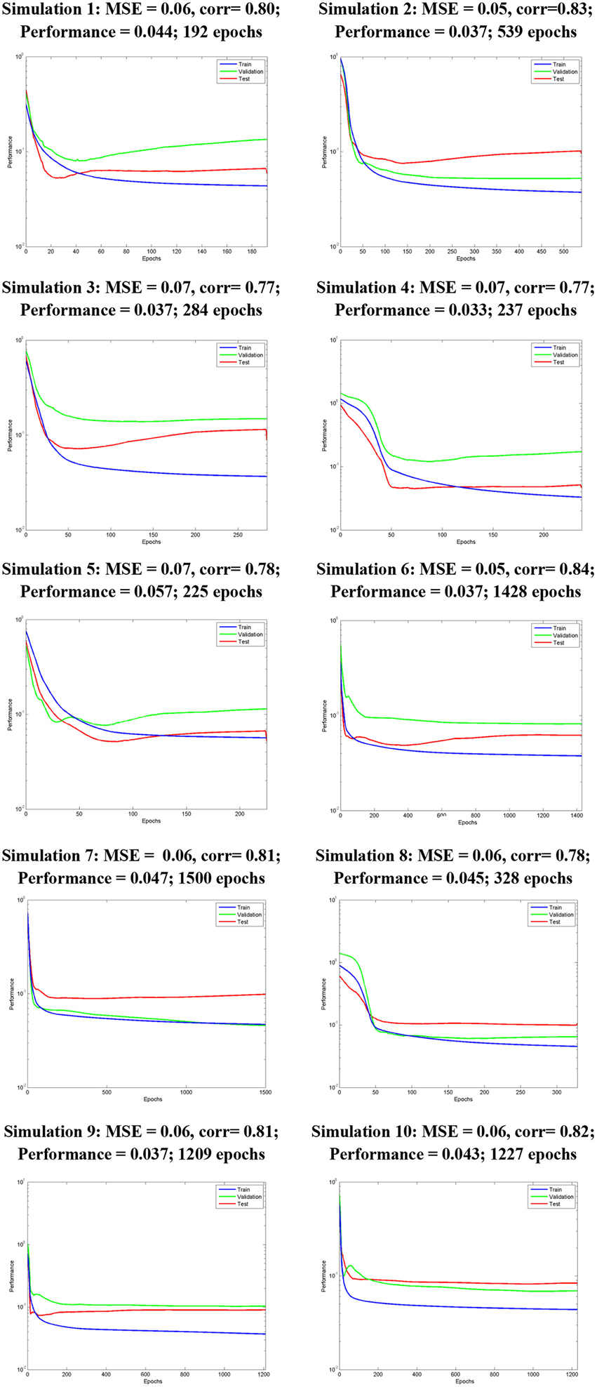
Figure 7. Simulations of the ANN model during the present climate period (1963–2003). In y-axis is the performance of each simulation divided in train (blue line), validation (green line), and test (red line) during different epochs (x-axis).

The simulation 2 shows the best performance and estimated generalization error MSE = |0.05| and correlation coefficient of 0.83 (Figures 7, 8). Although the values of MSE = |0.05| and corr = 0.84 in the simulation 6 it performance is not better than the simulation 2 which compromises the downscaled values. The explanation is that the purpose of training is to reduce the MSE to a low value using the few epochs as possible. The performance in simulation 6 is reached in 1426 epochs that is much long than in simulation 2 and also the respective test set (red line) is worst. Also, the variability of the output dataset obtained in the simulation 2 is better learned than in the simulation 6 (not shown). The Figure 8 shows the cross-validation used to validate the network performance. This means that the network output with respect to target (observed daily precipitation during FMA season of 1963–2003 period over the north of the NEB) for training, validation and test datasets. The equation Output = 0.7*target + −0.051 indicates how close the output is the target dataset. The fitting is reasonably good once the correlation coefficient is 0.83 and 70% of variability in output is explained by the target dataset The value of 0.051 represents the variability of the simulated output due the error term.

FIGURE 8

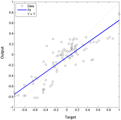
Figure 8. Cross-validation result of the best fit obtained in the Simulation 2 with MSE = 0.05 and corr = 0.83. The output simulated using as target the observed daily precipitation during FMA season and input the simulations of this variable from the four CMIP5 models in analysis during DJF season of 1963–2003 period over the north of the NEB is: Output = 0.7*target + −0.051.

The Equation 4 is the result of the MLR model used in the prediction of normalized daily precipitation during FMA season being represented by the relationship between the predictors: the normalized daily precipitation for DJF season observed and simulated by the CMIP5 models. The MSE obtained is |0.09| and the correlation between the predictors and predictand dataset is 0.70. The equation of the MLR derived model is shown as follow:

$\begin{array}{cc}\begin{array}{l}{\text{Prec}}_{FMA}=-0.17+0.22\ast {\text{Prec}}_{MIROC\_ESMDJF}\hfill \\ +0.22\ast {\text{Prec}}_{GFDL\_ESM2MDJF}+0.20\ast \hfill \\ {\text{Prec}}_{ObsDJF}-0.07\ast {\text{Prec}}_{CCSM4DJF}\hfill \\ +0.06\ast {\text{Prec}}_{CNRM\_CM5DJF}\hfill \end{array}& (5)\end{array}$

This equation defines that −0.17 is the constant value at which the fitted line crosses the y-axis representing the expected response when the predictors are zero. Each predictor (output of each one of the CMIP5 model) is weighted, and the weights denote their relative contribution to the overall adjustment. It is interpreted that the precipitation simulated from the MIROC_ESM and GFDL_ESM2M models during DJF season captures 22% of the variability of the observed daily precipitation during FMA season over the study region. Additionally, the observed daily precipitation during DJF season captures 20% of the variability in precipitation during FMA season. Only a few part of the observed daily precipitation during the rainy season is captured by the simulations of DJF season from the CCSM4 and CNRM_CM5 models. The equation indicates that MLR model not represents the suitable adjustment between the observed daily precipitation during the rainy season of FMA trimester and those predicted in 2 months before during the DJF season.

A comparison between nonlinear x linear methods illustrates that the downscaled values from the ANN model shows an improvement of 13% in terms of correlations coefficient values in comparison with the downscaled time series of the MLR model. This result is analyzed by subtracting the correlation coefficient value of 0.83 calculated between the observation and simulations values of the ANN model with those of the MLR model that is 0.70. Also, the ANN simulates a lesser generalized error of 0.05 in comparison with the obtained of the MLR model that is 0.09 and shows an improvement in the amplitude of the simulated time series.

The Figure 9 shows that ANN and MLR techniques exhibit the same positive tendency as in observation however there are deficiencies to predict the extreme values. Nevertheless, the best prediction of these extremes is found in ANN time series. This means that the MLR model is poorly suited to modeling the complex nonlinear relationships inherent in climate variables. Also, the ANN is more able to capture features of the interannual variability in the daily precipitation. In others, this is a useful tool to understanding of the main features of the precipitation in terms of large-scale atmospheric patterns.

FIGURE 9

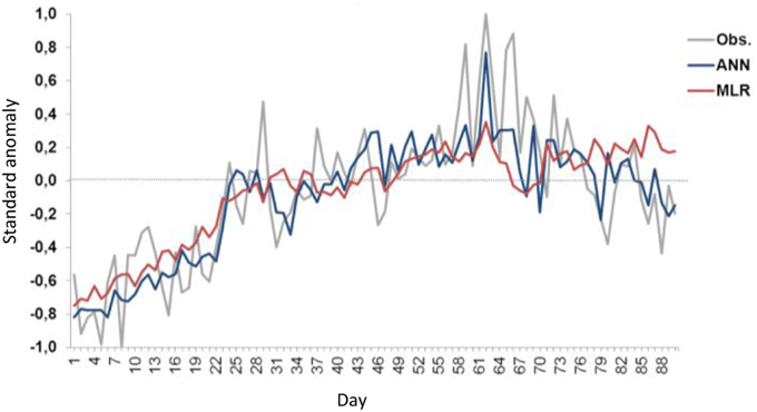
Figure 9. Comparison between the observed (gray line) and simulated daily precipitation by the ANN (blue line) and MLR (red line) models during FMA season of the 1963–2003 period over the north of the NEB.

The plot of the predictand bias (the simulated predictand values minus the observed values) shows that the distribution of errors with values close to zero being more frequent for nonlinear method than linear method (Figures 10A,B, respectively). It suggests that the ANN model is powerful to resolve the physical processes that are nonlinear in the precipitation dataset. However, the refinement methods show a tendency to underestimate high values of precipitation and to overestimate the low ones.

FIGURE 10

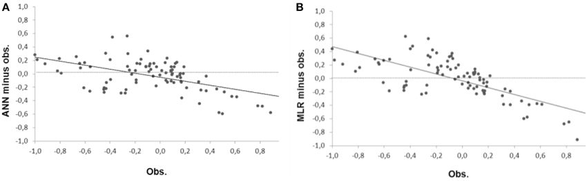
Figure 10. Bias comparison between the simulated daily precipitation by the ANN (A) and MLR (B) models during FMA season of the 1963–2003 over the north of the NEB.

Through the box-plots is shown that the median is similar in the observed and the two downscaled times series (Figure 11). However, the dispersion is best represented in the ANN than in MLR model when compared to the observations. Also, the MLR has a considerably lesser symmetric distribution of values in the predictand time series with a negative tail and more outliers indicating values with an abnormal distance from the other. The downscaled times series show a decreasing of the variance compared to the observations that is also indicated in Figure 9. According the previous results it suggested that the MLR has no skill in simulating the present-day climate over the region probability due the non-linearity imposed between the input and output data. Based on this, we decided to use the ANN method in the next analyses for the future climate.

FIGURE 11

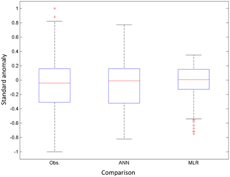
Figure 11. Box-plots comparison between observed and simulated daily precipitation by the ANN and MLR models during FMA season of the 1963–2003 period over the north of the NEB.

Future Climate

In the simulations for the future climate scenario we used the same ANN topology as those used in simulations for the present climate. The details about the design of the experiments are described in Section Results. We emphasize that the network projections criteria is different from those introduced in Boulanger et al. (2007). By comparing the 2055–2095 with the 1963–2003 periods is observed that all models project a positive tendency of daily precipitation over the north of the NEB (Figures 12A–C). An exception is found in the MIROC_ESM runs that projected a negative tendency and change from positive to negative on the rainy pattern (Figure 12D).

FIGURE 12

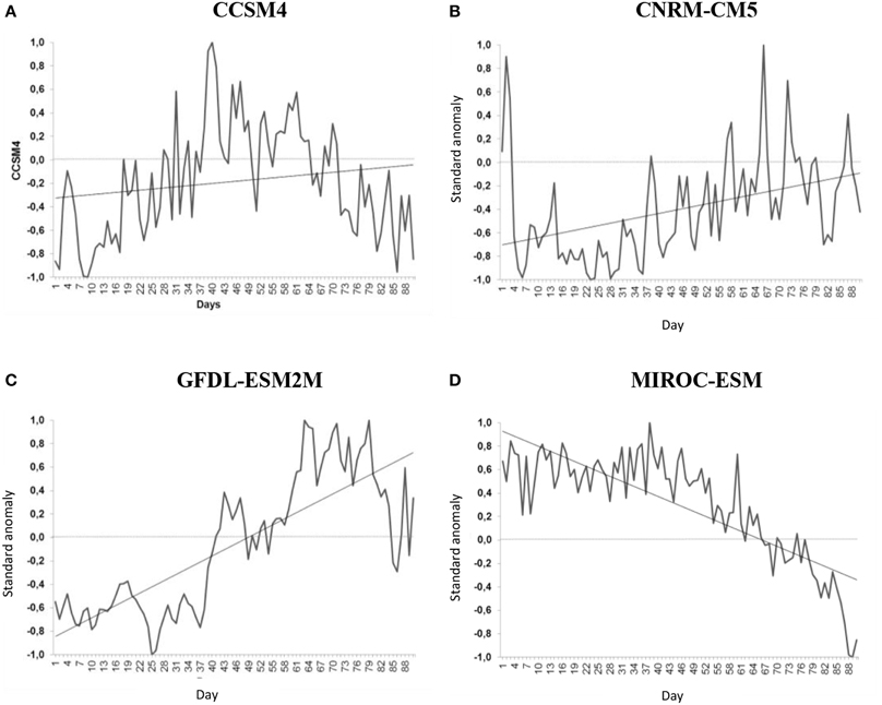
Figure 12. Projections of the daily precipitation on the future climate during FMA season of 2055–2095 period over the north of the NEB simulated by the CMIP5 models: (A) CCSM4, (B) CNRM_CM5, (C) GFDL_ESM2M, (D) MIROC_ESM.

The changes on the future climate projected by CMIP5 models for the 2055–2095 periods are validated with those obtained indirectly through the ANN model. The baseline is the predictand time series previously simulated for the present climate during the 1963–2003 period as shown in Section Present Climate. The best simulation results displayed in Figure 13 reached the MSE = 0.02 and correlation of 0.88 between the predictors and predictand datasets (Figure 13A). The result of the cross-validation Output = 0.74*target + −0.02 is interpreted as 74% variability of the output dataset is captured by all models and the uncountable part related to MSE = 0.02 is due the error in simulation. It means that the ANN model performs well in calibrating the climate model precipitation projections. The low MSE value may represent the local forcing as topography and local atmospheric processes that are smoothed in GCMs simulations due their low-resolution grid. We suggest the linear response that favors the relative high skill in predictability over the NEB in comparison with others regions of Brazil as mentioned in Introduction may be compromised when the models are forced by the greenhouse gas forcing RCP8.5. This suggests the importance of the RCP8.5 in change the large scale for the 2055–2095 periods. In Figure 13B the changes projected by ANN model exhibits near similar tendency as in GFDL_ESM2M model although the lower amplitudes.

FIGURE 13

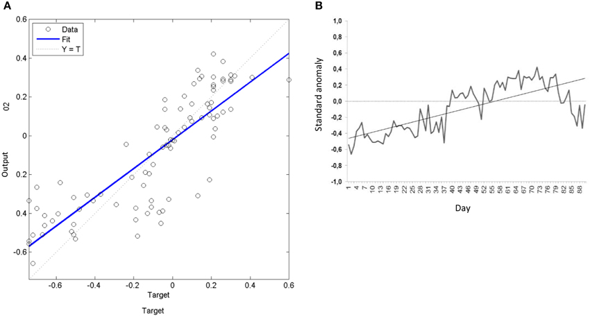
Figure 13. Results of the future climate change scenario simulation during FMA season of the 2055–2095 period of the ANN model: (A) Cross-validation result from the best fit with MSE = 0.02 and corr = 0.84. The output simulated using as target the simulated daily precipitation during FMA season from the ANN model and input the simulations of this variable from the four CMIP5 models in analysis during FMA season of 2055–2095 period over the north of the NEB is: Output = 0.74*target + −0.02. The letter (B) exhibits the respective time series.

The Table 4 shows the comparison through the correlation coefficient among the projected pattern from the ANN model and those from the CMIP5 models. It is clear that the ANN projection is more influenced by the GFDL_ESM2M response to RCP8.5 forcing. This model also shows a moderate correlation among the normalized daily precipitation during DJF and FMA seasons during the 1963–2003 period as seen in Figure 4 and Table 3. However, in analysis of the Figure 6 the mean structure of the ITCZ is better simulated in CCSM4 model that also show moderate correlation as displayed in Table 3. It suggests that a model may present a better simulation than another for the present-day climate but poorly respond to greenhouse gas forcing.

TABLE 4

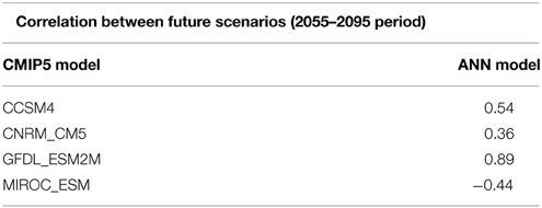
Table 4. Correlation between the future scenarios for the 2055–2095 period projected direct from the CMIP5 models and indirect from the ANN model.

The results reinforce that serious uncertainty are still persists since the CMIP3 model version in projections of equatorial precipitation as an expected consequence of global climate change. Ceppi et al. (2013) and some references therein explained that the hemispheres not heat evenly: the north hemisphere warm more swiftly than the south and this imbalance will have a consequent effect on the structure of the ITCZ. This fact underscores the importance of studies as the present here by applying statistical downscaling approach to improve the estimation of the variability to the GCMs outputs.

Discussions

Regarding the complex task that the numerical models in reproduce the precipitation some questions are addressed in this study.

Are the CMIP5 Models Able to Reproduce the Main Rainy Season Over the North of the NEB During the Present Climate?

No, from the four CMIP5 models analyzed there is a high dispersion of the daily precipitation over the north of the NEB justifying the use of downscaling methods. Overall, the differences between the models are reflected mainly in the mean and variability values of the daily precipitation over this region. The simulated daily precipitation by the CCSM4, GFDL_ESM2M, and MIROC_ESM models during DJF season are most correlated with the observed daily precipitation during FMA season. The correlations are of 0.54, 0.66, and 0.66, respectively. These correlations are explained by deficiencies shown in configuration of the anomalies of SST along the Equatorial Atlantic Ocean that result in anomalies in simulated daily precipitation over the north of NEB. Only the CCSM4 model displays a slightly reasonable agreement with the observations.

Regarding this aspect a comparison between the nonlinear (ANN) and linear method (MLR) to identify the one most suitable for the analysis of daily precipitation is made. No additional post-processing is applied on the downscaled outputs and the statistical methods show a decreasing of the variance in the predictand time series. Such feature is commonly encountered in the results of the application of statistical downscaling in climate research (Silva and Mendes, 2013; among others).

What is the More Adequate Statistical Downscaling Approach to Improve the Model Simulations During the Present Climate: the Artificial Neural Network (ANN) or the Multiple Linear Regression (MLR)?

We compared the relative performance of ANN and MLR models in improve the normalized daily precipitation during FMA season over the north of the NEB derived from observed and the CMIP5 outputs during DJF 1963–2003 period. The comparison between the methods is based in analysis of the Mean Squared Error (MSE), the linear correlation coefficient and the variability of the downscaled time series.

The nonlinear downscaling with ANN is potentially promising method of improvement of the explained variance of dataset than linear downscaling with MLR. The temporal downscaling through the ANN appears relatively efficient in correct part of the deficiencies in CMIP5 runs though the improvement of the large scale observed patterns. In terms of correlation coefficient values the improvement is of 13% between the predictors and predictand values from the ANN model compared to those from the MLR model. Also, the estimated errors and the amplitude of downscaled time series is best performed by ANN model.

Which One of These Statistical Models is More Appropriate to Project Future Scenarios of Climate Change Based on CMIP5 Runs?

Excluding the MIROC_ESM model the others ones are relatively coherent in comparing their 2055–2095 climate scenarios pattern over the north of the NEB. They have a tendency of increase of the daily precipitation projected. The projections for the FMA season derived directly from the mean grid box precipitation simulated from the CMIP5 models are compared with those obtained indirectly through ANN method. The baseline is the predictand downscaled for FMA time series. The climate scenario projected by ANN model indicates that the unaccounted explained variance is |0.02| that is the lower possible and corresponding to local forcings that will not change in future warmer climate (Trigo and Palutikof, 2001). This local forcing may be associated with the topography and local convection that are not well incorporated in the numerical models but influence the occurrence of precipitation. It may be suggested that the heavy-emission scenario of CO₂ in RCP8.5 is an important forcing of large-scale circulation for the 2055–2095 period. A comparison of the precipitation change projected from the ANN and those from the CMIP5 models indicated that the statistical model weights the CMIP5 runs according to their skill in simulating present-day climate. Similar characteristic is also found by the Boulanger et al. (2007) by comparing the 2076–2100 SRES A2 annual mean precipitation change projected by the ANN with those simulated by the seven models from the IPCC AR4.

Through the obtained results we suggest that the ANN method is an important tool to allow the establishment of complex relationship between large-scale and local climate over the north of the NEB. The complex relationship in the precipitation pattern over this region refers to the influence of local and remote forcing's related to SST variability. The purpose of this study is to emphasize that the ANN method that is used in many operational centers around the world in improvement of the predictability of numerical models needs more studies and applications in Brazil.

Furthermore the similar methodology as the present here will be carry out in analysis of the temporal and spatial dependence of these results with those for the east and south grid boxes over the NEB. The east and south of the NEB are regions with stronger nonlinearity compared with the north region and it is possible that ANN results may vary according to the regions particularities. Another important feature that will be investigated is the improvement when the local forcing, as the microclimate, will be included as predictors in addition with the precipitation simulated by the CMIP5 models.

Funding

This work received financial support from the “Coordenação de Aperfeiçoamento de Pessoal de Nível Superior – CAPES” during the post-doctoral research at Post-Graduate Program in Climate Science PPGCC-UFRN/Brazil.

Conflict of Interest Statement

The authors declare that the research was conducted in the absence of any commercial or financial relationships that could be construed as a potential conflict of interest.

Acknowledgments

We thank the two anonymous reviewers that provided relevant suggestions to improve the quality of the manuscript and the “Coordenação de Aperfeiçoamento de Pessoal de Nível Superior–CAPES” for providing the financial support. We are also thankful to researchers Brant Liebmann and Dave Allured for providing the observational South America 24 gridded precipitation dataset, the Program for Climate Model Diagnosis and Intercomparison (PCMDI) and the Working Group on Coupled Modelling (WGCM) for availability of the CMIP5 model dataset and the International Research Institute for Climate and Society for providing the IRI/LDEO Climate Data Library.

References

Biasutti, M., Battisti, D. S., and Sarachik, E. S. (2003). The Annual Cycle over the Tropical Atlantic, South America, and Africa. J. Climate 16, 2491–2508. doi: 10.1175/1520-0442(2003)016<2491:TACOTT>2.0.CO;2

CrossRef Full Text | Google Scholar

Boulanger, J. P., Martinez, F., and Segura, E. C. (2007). Projection of future climate change conditions using IPCC simulations, neural networks and Bayesian statistics. Part 2: precipitation mean state and seasonal cycle in South America. Clim. Dyn. 28, 255–271. doi: 10.1007/s00382-006-0182-0

CrossRef Full Text | Google Scholar

Cardoso, A. O., and da Silva Dias, P. L. (2004). Variabilidade da TSM do Atlântico e Pacífico e temperatura na cidade de São Paulo no inverno. Braz. J. Meteorol. 19, 113–122 (Available in Portuguese). Available online at: http://www.rbmet.org.br/port/revista/revista_dl.php?id_artigo=78&id_arquivo=75

Ceppi, P., Hwang, Y. T., Liu, X., Frierson, D. M., and Hartmann, D. L. (2013). The relationship between the ITCZ and the Southern Hemispheric eddy-driven jet. J. Geophys. Res. Atmos. 118, 5136–5146. doi: 10.1002/jgrd.50461

CrossRef Full Text | Google Scholar

da Silva, G. A. M., Drumond, A., and Ambrizzi, T. (2011). The impact of El Niño on South American summer climate during different phases of the Pacific Decadal Oscillation. Theor. Appl. Climatol. 106, 307–319. doi: 10.1007/s00704-011-0427-7

CrossRef Full Text | Google Scholar

Gardner, M. W., and Dorling, S. R. (1998). Artificial neural networks (the multilayer perceptron)-a review of applications in the atmospheric sciences. Atmos. Environ. 32, 2627–2636. doi: 10.1016/S1352-2310(97)00447-0

CrossRef Full Text | Google Scholar

Grodsky, S. A., and Carton, J. A. (2003). Intertropical Convergence Zone in the South Atlantic and the equatorial cold tongue. J. Climate 16, 723–733. doi: 10.1175/1520-0442(2003)016<0723:TICZIT>2.0.CO;2

CrossRef Full Text | Google Scholar

Hastenrath, S., Wu, M. C., and Chu, P. S. (1984). Towards the monitoring and prediction of Northeast Brazil droughts. Q. J. Roy. Meteorol. Soc. 110, 411–425. doi: 10.1002/qj.49711046407

CrossRef Full Text | Google Scholar

Janowiak, J. E., and Xie, P. (1999). CAMS_OPI: A Global Satellite-Rain gauge merged product for real-time precipitation monitoring applications. J. Climate. 12, 3335–3342.

Google Scholar

Johnson, B., Kumar, V., and Krishnamurti, T. N. (2012). Rainfall anomaly prediction using statistical downscaling in a multimodel superensemble over tropical South America. Clim. Dyn. 43, 1731–1752. Available online at: http://diginole.lib.fsu.edu/cgi/viewcontent.cgi?article=6524&context=etd

Kayano, M. T., and Andreoli, R. V. (2004). Decadal variability of northern northeast Brazil rainfall and its relation to tropical sea surface temperature and global sea level pressure anomalies. J. Geophys. Res. (1978–2012). 109. doi: 10.1029/2004JC002429

CrossRef Full Text | Google Scholar

Liebmann, B., and Allured, D. (2005). Daily Precipitation Grids for South America. Bull. Am. Meteorol. Soc. 86, 1567–1570. doi: 10.1175/BAMS-86-11-1567

CrossRef Full Text | Google Scholar

Mendes, D., and Marengo, J. A. (2010). Temporal downscaling: a comparison between artificial neural network and autocorrelation techniques over the Amazon Basin in present and future climate change scenarios. Theor. Appl. Climatol. 100, 413–421. doi: 10.1007/s00704-009-0193-y

CrossRef Full Text | Google Scholar

Mendes, D., Marengo, J. A., Rodrigues, S., and Oliveira, M. (2014). Downscaling statistical model techniques for climate change analysis applied to the Amazon region. Adv. Artif. Neural Syst. 2014:595462. doi: 10.1155/2014/595462

CrossRef Full Text | Google Scholar

Misra, V. (2004). A Diagnosis of Skill in an AGCM over Northeast Brazil. Cent. Ocean-Land Atmos. Stud. 171. Available online at: ftp://grads.iges.org/pub/ctr/ctr_171.pdf

Moss, R. H., Edmonds, J. A., Hibbard, K. A., Manning, M. R., Rose, S. K., Vuuren, D. P., et al. (2010). The next generation of scenarios for climate change research and assessment. Nature 463, 747–756. doi: 10.1038/nature08823

PubMed Abstract | Full Text | CrossRef Full Text | Google Scholar

Ramírez, M. C., Ferreira, N. J., and Velho, H. F. C. (2006). Linear and nonlinear statistical downscaling for rainfall forecasting over southeastern Brazil. Weather Forecast. 21, 969–989. doi: 10.1175/WAF981.1

CrossRef Full Text | Google Scholar

Riahi, K., Gruebler, A., and Nakicenovic, N. (2007). Scenarios of long-term socio-economic and environmental development under climate stabilization. Technol. Forecast. Soc. Change 74, 887–935. doi: 10.1016/j.techfore.2006.05.026

CrossRef Full Text | Google Scholar

Riahi, K., Shilpa, R., Volker, K., Cheolhung, C., Vadim, C., Guenther, F., et al. (2011). RCP 8.5— A scenario of comparatively high greenhouse gas emissions. Clim. Change 109, 33–57. doi: 10.1007/s10584-011-0149-y

CrossRef Full Text | Google Scholar

Richter, I., Xie, S. P., Behera, S. K., Doi, T., and Masumoto, Y. (2014). Equatorial Atlantic variability and its relation to mean state biases in CMIP5. Clim. Dyn. 42, 171–188. doi: 10.1007/s00382-012-1624-5

CrossRef Full Text | Google Scholar

Rodrigues, R. R., Haarsma, R. J., Campos, E. J. D., and Ambrizzi, T. (2011). The impacts of inter-El Niño variability on the tropical Atlantic and Northeast Brazil climate. J. Clim. 24, 3402–3422. doi: 10.1175/2011JCLI3983.1

CrossRef Full Text | Google Scholar

Sajikumar, N., and Thandaveswara, B. S. (1999). A non-linear rainfall-runoff model using artificial neural network. J. Hydrol. 216, 32–55. doi: 10.1016/S0022-1694(98)00273-X

PubMed Abstract | Full Text | CrossRef Full Text | Google Scholar

Silva, G. A., Dutra, L. M., da Rocha, R. P., Ambrizzi, T., and Leiva, É. (2014). Preliminary analysis on the global features of the NCEP CFSv2 seasonal hindcasts. Adv. Meteorol. 2014:695067. doi: 10.1155/2014/695067

CrossRef Full Text | Google Scholar

Silva, G. A. M., and Mendes, D. (2013). Comparison results for the CFSv2 hindcasts and statistical downscaling over the northeast of Brazil. Adv. Geosci. 35, 79–88. doi: 10.5194/adgeo-35-79-2013

CrossRef Full Text | Google Scholar

Siongco, A. C., Hohenegger, C., and Stevens, B. (2014). The Atlantic ITCZ bias in CMIP5 models. Clim. Dyn. 1–12. doi: 10.1007/s00382-014-2366-3

CrossRef Full Text | Google Scholar

Smith, T. M., Reynolds, R. W., Peterson, C. T., and Lawrimore, J. (2008). Improvements to NOAA's Historical Merged Land-Ocean Surface Temperature Analysis (1880-2006). J. Clim. 21, 2283–2296. doi: 10.1175/2007JCLI2100.1

CrossRef Full Text | Google Scholar

Taschetto, A. S., and Ambrizzi, T. (2012). Can Indian Ocean SST anomalies influence South American rainfall?. Clim. Dyn. 38, 1615–1628. doi: 10.1007/s00382-011-1165-3

CrossRef Full Text | Google Scholar

Trigo, R. M., and Palutikof, J. P. (2001). Precipitation scenarios over Iberia: a comparison between direct GCM output and different downscaling techniques. J. Clim. 14, 4422–4446. doi: 10.1175/1520-0442(2001)014<4422:PSOIAC>2.0.CO;2

CrossRef Full Text | Google Scholar

Xie, S. P., and Carton, J. A. (2004). Tropical Atlantic variability: Patterns, mechanisms, and impacts. Earth Clim. 121–142. doi: 10.1029/147GM07

CrossRef Full Text | Google Scholar