Modeling the Effects of Soil Variability, Topography, and Management on the Yield of Barley

Introduction

Modeling plant growth has become an increasing part of agriculture practice, e.g., in decision making, planning, and the consideration of risks. During the last 30 years, crop growth modeling has changed dramatically from simple input-output relationships to highly professional activities with submodels for agricultural meteorology including different CO₂-concentrations, water retention and flow, turnover of C, N, and further parameters.

In this connection Bossel (1994) emphasized the meaning of gray box modeling. This forms a hybrid between the structural and behavioral models. The mixed form is particularly common since the effect structure and parameters of real systems can often only be determined incompletely. An attempt is made to present the impact structure to the best of its knowledge in such a way that the model exhibits a qualitatively correct behavior. Unknown model parameters are then adjusted so that the model also numerically matches the observed behavior of the original [Expert-N (Priesack, 2006), HERMES (Kersebaum and Beblik, 2001), DAISY (Abrahamsen and Hansen, 2000)].

Traditionally, crop modeling is derived from conventional experienced-based agronomic research, where yields were related to some defined variables. The advantage of black-box-modeling is that costly causal analysis can be dispensed. Despite the simplicity, this description of crop production with regressions and similar statistical procedures has until today had a wide application, e.g., in the derivation of fertilization recommendations and the desired level of liming.

Decisions in practical plant production in Germany are predominantly based on such simple models. These are components of the recommendations of the Association of German Agricultural Analytical and Research Institutes (VDLUFA). The VDLUFA models for nutrient dynamics are based on the examination of the soil and the balancing of nutrient supply and discharge. This organization acts as a political advisor for federal state ministries (http://vdlufa.eu/index.php, 2017)¹ and provides farmers with the appropriate fertilizer recommendations after soil analyses.

Further areas of application are the evaluation of field experiments (fertilization, liming, pest management, cover crop, tillage/no-tillage) which is addressed in this work. Here, the application of regressions and related statistical procedures have provided some qualitative understanding of the interaction of independent variables as well as the meaning for the dependent variable “yield.”

Therefore, investigations were carried out on a long-term fertilizer experiment with the treatments “six different forms of N-fertilizer” and “three levels of nitrogen fertilization (including control plots).”

The most common practice to evaluate such experiments is analysis of variance with the factors N-fertilizer and fertilization level. However, the variability of the soil and of the topography indicated a marked influence on the yield level. For that reason, soil conductivity (EC_a), relief parameters, and coordinates were used as proxies for site conditions. The advantage of these variables is that they are relatively easy to carry out and represent inexpensive measurements.

EC_a, topographical parameters, and coordinates have no direct relationship to the growth and yield of plants, but the spatial variation of these parameters is partly correlated with soil properties that do affect crop productivity. Several studies have shown this connection (Jaynes et al., 1995b; Kitchen et al., 1999; Luchiari et al., 2000; Corwin et al., 2003; Lukas et al., 2009). The wide range of the application of EM38- EC_a are described in Heil and Schmidhalter (2017).

Kitchen et al. (1999) related EC_a to yield and found a significant correlation (boundary lines with R² > 0.25 on most areas), but climate, crop type, and specific field information was also necessary to explain the relationship. Fraisse et al. (2001) also used a combination of EC_a and topographic features to test their ability to describe yield variability. By dividing a field into four or five zones based on EC_a, slope, and elevation, 10 to 37% of corn and soybean yields were explained. Guretzky et al. (2004) tested the relationship of the relief parameter “slope,” EC_a, and legume distribution in pastures. The authors concluded that EC_a and slope were useful in selecting sites in pastures with higher legume yield and indicated its use in the site-specific management of pastures. Tarr et al. (2003) used groups of apparent conductivity and topographical parameters to divide with fuzzy-k clustering a heterogeneous pasture area into relatively homogeneous zones. The five derived subareas indicated significant differences in the target variables (i.e., organic matter, soil moisture, P, K, and pH).

Relief and soil properties are often strongly correlated to the processes of soil development, erosion, and sedimentation (Gerrard, 1981; Pennock and de Jong, 1987; Moore et al., 1993). At a site in Andalusia, Southern Spain, the organic carbon content in the northern position was higher than in the other topographical aspects (Lozano-García et al., 2016). Various authors described the important role of the topography (especially elevation, slope, and aspect) on the temperature and humidity regimes (Bale et al., 1998; Mohanty and Skaggs, 2001; Rech et al., 2001; Griffiths et al., 2009). Yang et al. (1998) and Bakhsh et al. (2000) found, with the help of GIS data, that topographic was related to yield.

The geographical position of an object is given by the high value and the right-hand value. By using these coordinates, each yield value of a plot is given a particular grid reference (Thöle, 2010).

Modeling these relationships was the main objective of this study. Our focus was on the following questions:

- Could the yields of barley (annual and perennial) be estimated using EC_a measurements, topographical parameters and Gauss-Krüger coordinates?

- Are there any predictors that are highly significant for barley yield at this location?

- What impact do fertilizer form and N-level have on yield in the models?

Materials and Methods

General Description, Site of the Dürnast Long-Term Experimental Field

The study area was ~0.31 ha in size, located 30 km north of Munich, Germany (4477221.13 E, 5362908.78 N) in the Tertiary landscape and is part of the long-term field experiments of the Chair of Plant Nutrition, Technical University of Munich (Heil and Schmidhalter, 2017).

The average annual temperature is 7.8°C, and the average annual precipitation is 810 mm (1971–2000).

The dominant soil material is Tertiary sediments with deposits of Pleistocene loess. The composition of the soil is a consequence of loess deposition and subsequent erosion. According to the German Soil Survey (Arbeitsgruppe Bodenkunde, 1994), fine-loamy Typic Udifluvent and fine-silty Dystric Eutrochrept are the dominant soil types. The main characteristics of the relief and soil parameters are listed in Table 1.

TABLE 1

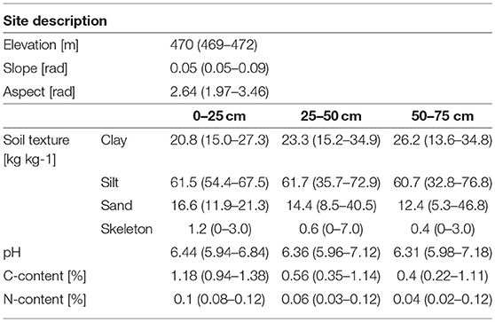
Table 1. Site description of the long term fertilization experiment in Dürnast (Heil and Schmidhalter, 2017).

Experimental Design

The ongoing was established in encompassing 11 years of barley cultivation (1981, 1984, 1987, 1990, 1993, 1996, 1999, 2002, 2008, 2011, and 2013). Fertilizer amount and form, crop rotation, and plot size of this experiment are listed in Table 2. Table 3 indicates the years of cultivation with barley, the cultivars and the number of replications. In Figures 1, 2, the layout of the experimental field is presented. Of note, calcium ammonium nitrate was tested twice. The control plots (no fertilization) were located within every row. Furthermore, after 2006, the experiment was reduced to four replications, identified as a-d (Figure 1).

TABLE 2

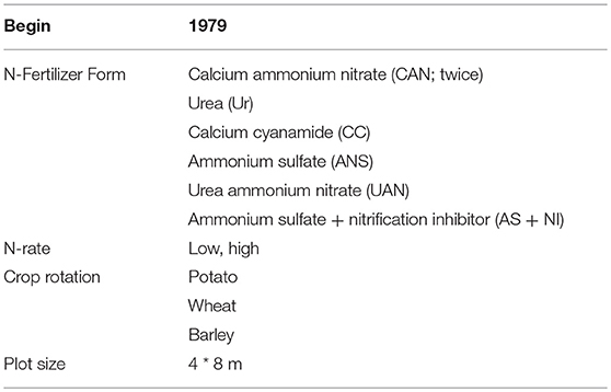
Table 2. Basic features of the long term N-fertilization experiment.

TABLE 3

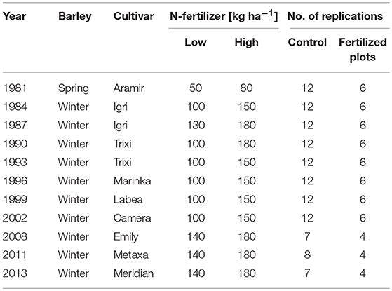
Table 3. Cultivars, amount of fertilizer, and number of replicates.

FIGURE 1

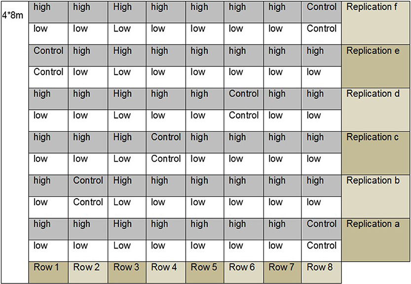
Figure 1. Schematic representation of the experimental area with the distribution of the fertilized and control plots per replication.

FIGURE 2

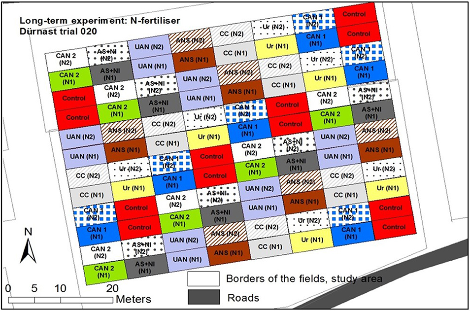
Figure 2. Arrangement of the experimental area with the distribution of the N-fertilizer forms (abbreviations, see Table 2) and the level of fertilization [low (N1), high (N2)].

Data Collection

For the prediction of the barley yield, the following independent variables were used:

(i) experimental cultivation parameters:

- fertilizer (control = 0, fertilizer no. 1–6) (Table 2),

- level of fertilization (control = 0, low = 1, high = 2) (Table 3);

(ii) EC_a (EM38-v, EM38-h, MK2-v-1.0m, MK2-h-1.0m, MK2-v-0.5m and MK2-h-0.5m); for explanations see section Apparent Electrical Conductivity (ECa)

(iii) parameters from digital topographic model; and

(iv) position in the middle of the plots (Gauß-Krüger coordinates).

Yield Data

As a dependent variable, the grain yield per plot was determined with a conventional plot combine harvester.

Apparent Electrical Conductivity (EC_a)

This conductivity was measured with the sensors EM38 and EM38-MK2 on April 1, 2011 in all possible configurations (vertical (v), horizontal (h) configuration) on the experimental field 020.

A detailed description and also a comparison of both devices are given in Heil and Schmidhalter (2015).

Based on the recommended practice for performing such measurements, soil water contents were near field capacity. This assumption was supported by data of the German weather service for the region (unpublished weather data of the station Freising). The EC_a values were standardized to electrical conductivity at a temperature of 25°C using the equation developed by Sheets and Hendrickx (1995). In the next step, the EC_a data were interpolated in 2-m grids using GIS software with experimental omnidirectional semi-variograms and ordinary kriging.

The end results were continuous maps of EC_a distributions (EM38-v, EM38-h, MK2-v-1.0, MK2-h-1.0, MK2-v-0.5, and MK2-h-0.5).

Digital Relief Model

Elevation grid data of approximately 400 ha of the area with a grid size of 2-m was obtained from the Agency for Digitization, High-Speed Internet, and Surveying (Munich). Additional topographic parameters were calculated with the software package System for Automated Geoscientific Analyses (SAGA², produced by Scilands GmbH Göttingen, www.scilands.de). Beside elevation the following variables were used as independent variables in the statistical derivations (Conrad et al., 2015):

elevation (ELEV) [m];

slope gradient (SG) [radian];

aspect (ASP) [radian];

upslope catchment area (CA) [m2];

topographical wetness index (TWI) [–];

plancurvature (PLC) [–];

profilecurvature (PRC) [–];

convergence (CON) [%];

LS-factor (LSF) [–];

channel network base level (CNBL) [–];

vertical distance to channel network (VDCN) [–];

valley depth (VD) [m] and

relative slope position (RSP) [–].

Construction of the Data Set for Calculations

For each plot position, parameters (Gauß-Krüger) were determined and EC_a as well as topographical parameters were averaged.

Yield values, experimental cultivation parameters, and the parameters listed above were combined into one data set.

From the beginning of the experiment in 1979 until 2006, each treatment had six replications. In 2007 the number of control plots was reduced from 12 to 8 and the number of fertilized replications was reduced from 12 to 8.

Statistical Analyses

The statistical analysis was carried out with the SPSS program of the manufacturer IBM (v 22.0). To achieve the aims of the experiment and answer the experimental question, statistical methods such as analysis of variance (ANOVA), analysis of covariance (ANCOVA), and linear regression (REG), were chosen (Kutner et al., 2005).

The theoretical model of REG is

$\begin{array}{l}{\text{Y}}_{\text{i}}={\beta }_0+{\beta }_1{\text{x}}_{\text{i}1}+{\beta }_2{\text{x}}_{\text{i}2}+\dots +{\beta }_{\text{p}}{\text{x}}_{\text{ip}}+{\text{e}}_{\text{j}}\end{array}$

where the dependent variable (y_i) represents the barley yield; x_i represents relief attributes, EC_a measurements, and fertilizer parameters; β_p is the empirical regression model coefficient; and e_j is the residual error component of the model.

For the models, the variables used were tested for normal distribution (0.05 significance level, Kolmogorov-Smirnov test with the significance correction according to Lilliefors) (Garson, 2012). Non-normally distributed variables were transformed.

The theoretical model of ANOVA is

$\begin{array}{l}F=\frac{variancebetweentreatments}{variancewithintreatments}\\ F=\frac{\frac{1}{l-1}}{\frac{1}{n-1}}\frac{S{S}_A}{S{S}_R}=\frac{\frac{1}{l-1}}{\frac{1}{n-1}*{\sum }_{i=1}^l*}\frac{*J{\sum }_{i=1}^J{(\overline{x_i}-\overline{x})}^2}{{\sum }_{j=1}^J{(\overline{x_{ii}}-\overline{x_i})}^2}\end{array}$

SS_A is the sum of squares of the treatments

SS_R is the sum of squares of the error

l is the number of treatments (no. of fertilizer form, N-fertilizer level = 2)

n is the number of cases (control plots and fertilized plots = 96)

$\overline{x}$ is the mean of the data set (mean of all 96 plots)

$\overline{x_i}$ is the mean of the i-group (mean of each single group)

i is the number of groups (=16 groups)

J is the number of measurements (=1, measurement in the case of multiannual mean yield)

j j-measurement (=1, first measurement in the case of multi-annual mean yield)

(Heil and Schmidhalter, 2017).

The analysis of covariance (ANCOVA) connects the properties of REG with the properties of ANOVA. ANCOVA combines the ANOVA model with one or more additional variables (covariates) that correlate with the target variable (Heil and Schmidhalter, 2017).

In the calculations for this study, the ANOVA was performed as follows:

$\begin{array}{l}y=\mu +Factor(N-level)+Factor(N-fertilizerform)\\ +Factor(N-level)*Factor(N-fertilizerform)+e\end{array}$

The extension of the ANCOVA procedure was as follows:

$\begin{array}{l}=\mu +Factor(N-level)+Factor(N-fertilizerform)\\ +Factor(N-level)*Factor(N-fertilizerform)\\ +\text{ ECa}+\text{relief }+\text{Position}+\text{e}\end{array}$

where y is the yield; μ is the mean of the yield; factor N-level and N-fertilizer form reflect the effects of quantity and form of the fertilizer; and e is the error term. The term relief includes the topographical parameters listed above. Position describes the Gauß-Krüger coordinates of the plots (Heil and Schmidhalter, 2017).

The evaluation of the models were carried out with the RMSD (root mean square difference) and the nRMSD (normalized root mean square difference):

$\begin{array}{l}RMSD={\left[1/N{\displaystyle \sum _{i=1}^{N(h)}}{(Z_{si}-Z_{si}^{*})}^2\right]}^{0.5}\end{array}$

where N represents the site, z_si represents the observed value, and ${\text{z}}_{\text{si}}^{*}$ represents the predicted value.

The nRMSD indicates the RMSD in relation to the mean of the observed values. Here nRMSD is expressed as a percentage, where lower values shows less residual variance.

$\begin{array}{l}nRMSD=\frac{RMSD}{\overline{z}}*100\end{array}$

The RMSD is a measure of the accuracy of the prediction calculation, and this value is small for an unbiased prediction.

Results

Modeling of Multi-Annual Means of Yield

The multi annual barley yields of control plots were just over 20 dt ha⁻¹ on average (see Figure 3), which was approximately between one third to half of the yield of the treatments with fertilization. The multi-annual barley yields showed a relatively comparable picture regarding the N-levels and the fertilizer forms. The plots with high fertilization did not produce considerably higher yields.

FIGURE 3

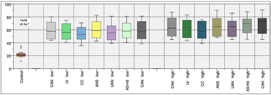
Figure 3. Multi-annual yields of barley (means and coefficients of variation of the years 1981–2013).

The map of the multi-annual yields (Figure 4) indicated a strong spatial increase (both control and fertilized plots) from the northwest corner to the south border (control plots: 14.7-23.6 dt ha⁻¹; low fertilized plots: 50.2-62.5 dt ha⁻¹; high fertilized plots: 55.2-68.2 dt ha⁻¹).

FIGURE 4

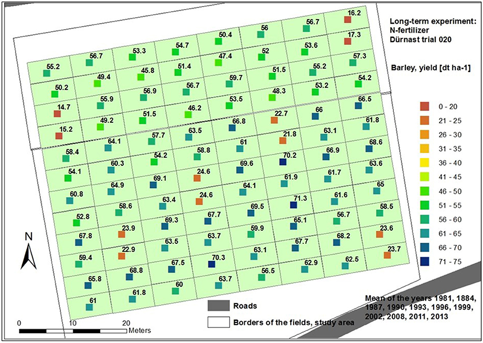
Figure 4. Georeferenced multi-annual yields of barley (plot wise means) of the years 1981–2013.

An opposite trend can be seen for the EC_a readings from both devices and for all configurations (Figures 5, 6). The gradient showed an increase of about 25 mS m⁻¹.

FIGURE 5

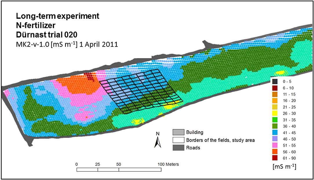
Figure 5. 3-dimemsial map of interpolated EC_a readings [mS m⁻¹] in a 2.m grid measured with MK2-v-1.0 and the borders of field experiment.

FIGURE 6

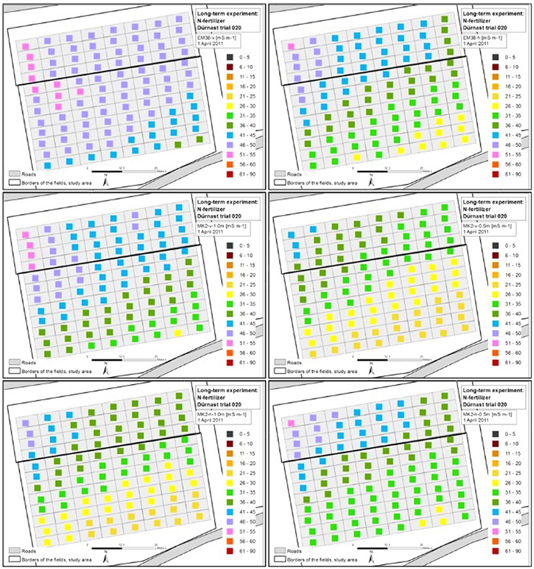
Figure 6. Plot wise EC_a readings (mS m⁻¹) from both devices EM38 and MK2 in the configurations vertical, horizontal, 0.5, and 1.0 m of the field experiment 020.

The average values were characterized by an increase from MK2-v-0.5m, MK2-h-1.0, MK2-h-0.5m, EM38-h, MK2-v-1.0m to EM38-v.

For a more detailed insight into the parameters which influence the yield, the calculations of the multi-annual as well as the annual data sets were divided into non-fertilized and fertilized data.

The modeling of the yield of the control plots was calculated with REG in two different ways (Table 4), at first with all continuous independent variables (Model 1) and at second only with EC_a (Model 2). In the first calculation, the significant variables were the upslope catchment area and EC_a MK2-h-0.5 with a R² = 0.83 and an RMSD of 1.26 dt ha⁻¹. However, the modeling of the yield was also satisfactory with only EC_a MK2-h-05as the predictor. Here, EC_a -MK2-h-0.5 could explain about 70% of the variation with an RMSD of 1.45 dt ha⁻¹.and a nRMSD of y only 7%.

TABLE 4

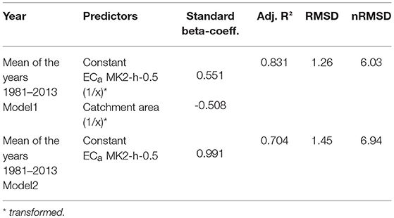
Table 4. Simulation of the yield of the control plots (means of the years 1981–2013) with REG (above: Model 1 predictors EC_a, relief, coordinate, below: Model 2 predictors EC_a), (further information see Supplementary Table 1).

The ANOVA procedure of the fertilized plots (Table 5) indicated that only a weak relationship was detected between yield and the factors fertilization level and fertilizer form. The modeling with ANCOVA delivered a significant improvement with the additional usage of EC_a as readings from the configuration MK2-h-0.5 (Table 6). Here both RMSD and also nRMSD were nearly halved.

TABLE 5

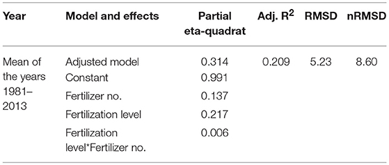
Table 5. Modeling of the yield (means of the years 1981–2013) with ANOVA with the factors fertilization level and fertilizer number (see also Supplementary Table 2 for further information).

TABLE 6

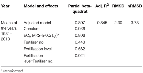
Table 6. Modeling of the yield (means of the years 1981–2013) with ANCOVA with the factors fertilization level and fertilizer number and the covariates EC_a, topographic parameters, and coordinates (further information is contained in Supplementary Table 3).

It was remarkable that in the ANOVA, the factor “fertilization form” was not significant, while in the ANCOVA the importance was highly significant (further information is given in Supplementary Tables 2, 3).

This multi-year evaluation does not allow to work out the yearly influence of barley varieties and also varying amounts of fertilizers (also within the fertilization levels). These calculations represent a yield average as influenced by the weather conditions of 11 years and the fertilizer forms and cultivar selection.

Modeling of Annual Yields

Overall, the annual yields of the control plots could be described very well by the calculated regressions (Table 7). Without the first year of investigation, the R² exceeded a value of 0.77. Within a range of 15–35 dt ha⁻¹, these values even reached coefficients of determination of 0.85. The RMSD varied between 0.5–1.6 dt ha⁻¹ and the nRMSD indicated values lower than 8.5%, without the year 1999 with a relatively low yield of 10.6 dt ha⁻¹. The main influencing parameters were MK2-EC_a, here as the configuration MK2-h-0.5 followed by the configuration MK2-v-1.0. The topographical parameters showed a more diverse picture with the variables PRC, PLC, CNBL, and CA.

TABLE 7

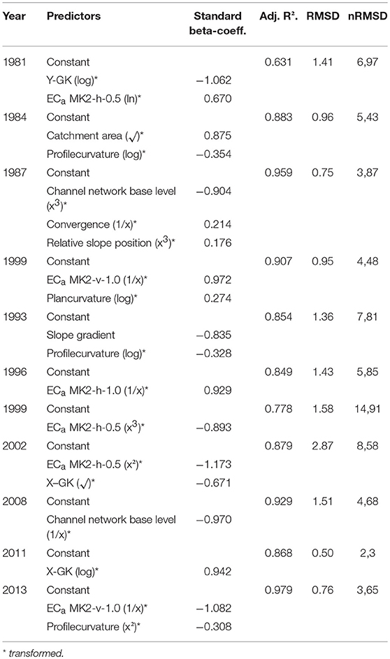
Table 7. Simulation of the annual yield from 1981–2013 with REG of the control plots and the independent variables EC_a, relief, and coordinates (further information is contained in Supplementary Table 4).

The modeling of the annual yields of the fertilized plots (Table 8) with ANOVA strongly indicated fluctuating values for R², RMSD, and nRMSD without a consistent relation to yield. Very often, the factors fertilizing level and fertilizer form both had significant effects on the yield. However, this was not observed in 1987 for the fertilizing level and in 1981 and 2002 for the effect of the fertilizer form. The accuracies of the calculations were higher when the fertilizer form was significant.

TABLE 8

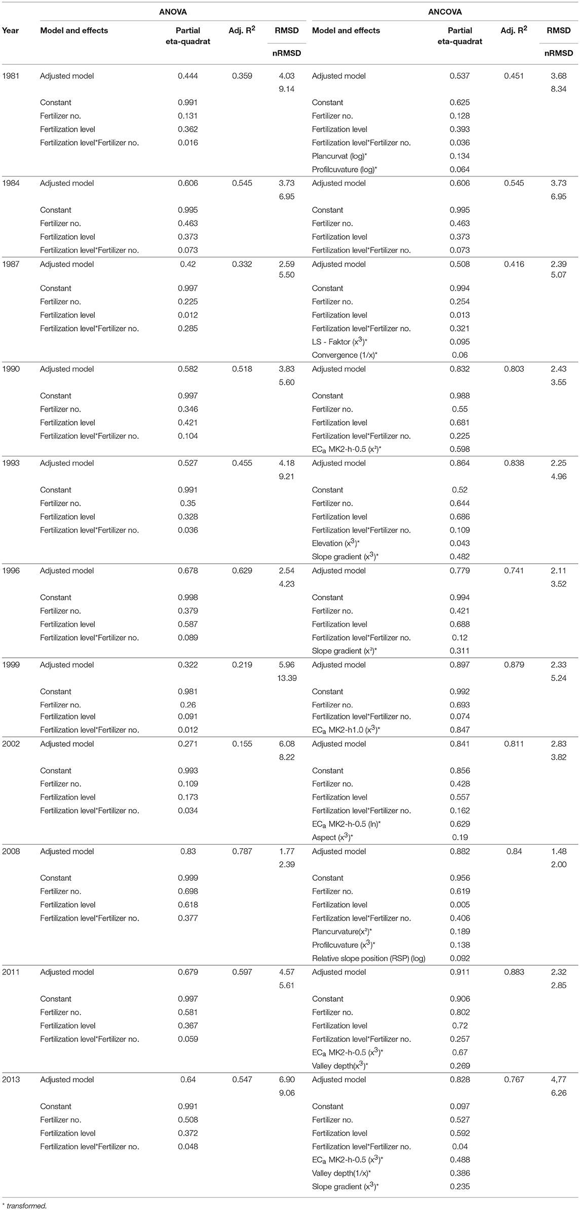
Table 8. Simulation of the annual yield from 1981–2013 with ANOVA and ANCOVA (further information is given in Supplementary Table 5).

Without the first 3 years, the modeling with the ANCOVA procedure produced a marked improvement with R² amounting to 0.74. In 1999 and 2011, the highest R² among the years from 1981 to 2013 was depicted and in the case of RMSD this observation held true for the years 1996 and 2008. The variation of the nRMSD within the years 1987 to 2011 was lower than 5.3%.

The overall evaluation indicated that the nitrogen level and nitrogen form were the dominating predictors. Only in 1981 was the nitrogen form not significant, and in 1987 and 2008, the level was also less important.

In some years, the effect size after partial eta² was greater regarding the factor fertilizer form than the factor fertilization level (1984, 1987, 1993, 1999, 2008, 2011, and 2013). Furthermore, the EC_a-readings and topographical parameters enhanced the quality of the relationships. The dominating EC_a -configuration was MK2-h-0.5. The factor-group topographical parameters were built by CA, VP, PLC, PRC, and CON.

Discussion

Experienced-based agronomic research where crop yields are related to a single or more parameters is traditionally one of the bases of agricultural decision making. Crop yields are expressed as mathematical functions of defined parameters (Geesing et al., 2014).

In contrast, the evaluation of the long-term field experiment “N-forms, 020 Dürnast” showed that a combination of easily and inexpensively obtained parameters was the base for a sufficiently precise derivation of crop yields. However, other independent variables might also be applicable, e.g., remote sensing data and other soil sensing data [spectral reflectance, resistance, or gamma measurements (Robinson et al., 2009)].

Another conclusion can also be drawn. The variables apparent conductivity, topographical features, and coordinates are either stable or relatively comparable over time, which also permits ex-post evaluations of long-term field experiments (Heil and Schmidhalter, 2017).

The disadvantages of this type of modeling are that the assessment of risks that are the consequence of single influencing factors, e.g., climatic perturbations and diseases, cannot a priori be integrated. Given the static character of the models, any adaptation to changed environmental conditions is not possible (Kravchenko et al., 2005). As well not all differences in soils that account for yield differences can be assayed by proximal soil sensing as used in this study. Furthermore, this methodology does not allow the evaluation of the different cultivars in the model design (eight cultivars in 11 years of cultivation).

Despite these limitations, the fitted models mostly agreed well with the observed variation in barley yields. The RMSD values in individual years are within acceptable limits. Relatively high R²-values >0.74 indicated that in most years, crop yield was largely governed by variables accounted for in the models. However, it is necessary to consider that yield can also be affected by other factors. Other influencing factors like climate, pests, diseases, and human activities can cause local variations in predicted crop yields. This poses a limitation to this sort of modeling.

The present work indicates that,

(i) EC_a exerted a significant influence in most of the derivations, mainly in the configuration MK2-h-0.5. This influence was exclusively negative (Figure 7).

(ii) The weight of relief and EC_a demonstrated that the growing conditions were not homogeneous in this relatively small field.

(iii) The selected topographical parameters contributed in different forms the parameter slope of the field in different derivations.

(iv) Fertilization factors dominated the ANCOVA calculations in the years 1981, 1984, 1987, 1993, 2008, 2011, and 2013. In five of the investigated years, the nitrogen fertilization form exceeded the importance of the nitrogen level (years 1984, 1987, 1999, 2008, and 2011).

FIGURE 7

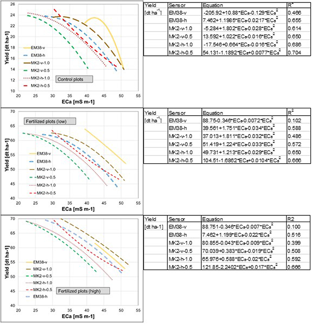
Figure 7. Relationships between EC_a and yields for the control and the fertilized plots with low and high levels of N fertilizer.

Relationships between EC_a and yield have often been described in the literature and the direction of the correlation is increasingly being evaluated.

Robinson et al. (2009) gave a detailed insight into such relationships for sites in Victoria, Australia. However, the multi-year measurements of EC_a and yield delivered an inconsistent picture. Significant influences were found for all measurements, but with different directions. (1) Decreasing yield was combined with increasing EC_a -v on areas with increasing clay content. (2) Positive trends of EC_a and yield were found in areas with better water supply in high and moderate yield zones.

In an investigation on claypan soil, Sudduth et al. (1995) described in a dry year a negative correlation. Contrary results with also negative relationships with corn and soybean, but in a wet year in a topographically highly variable landscape were described by Jaynes et al. (1995a). However, in both studies, no significant relationships were observed in years with more normal precipitation.

In the current investigation, the relationships were also negative. High EC_a -readings corresponded with low yields. Heil and Schmidhalter (2017) indicated, that lower EC_a values were combined with lower elevations and also higher catchment areas and more silty soils (silt: 67 kg kg⁻¹; clay: 16 kg kg⁻¹; sand: 16 kg kg⁻¹; skeleton: 2 kg kg⁻¹; near the southern border). On the other hand, higher EC_a readings were measured in soils at higher elevations with more clay (clay: 26 kg kg⁻¹; silt: 56 kg kg⁻¹; sand: 17 kg kg⁻¹; skeleton: 3 kg kg⁻¹; near the northern border). Additionally, soils with a lower EC_a readings had higher contents of N and C (Heil and Schmidhalter, 2017).

However, the negative relationships between the devices and their configurations differed. In all cases, the R² of EM38-v indicated the lowest level and MK2-h-0.5 the highest values. It was noticeable that configurations which showed the conductivities of the more shallow soil depths were better retrievable. From this is deducible that mainly the subsurface readings were necessary for the modeling.

Obviously soil factors influenced the spatial growth of the crop. Two factors most likely account for such effects, root growth and water availability. Soil factors which have the largest effect on root growth are pore distribution, penetration resistance, and also water and nutrient availability (Hoad et al., 2001). It was assumed that the growing conditions were less favorable from the south to the north-west border. The field management within the N-fertilization was the same across the whole field, so that operations that may influence rooting (rotation, variety choice, cultivations, sowing rate, sowing date, and nitrogen fertilization timing) did not differ. A further explanation is the depiction of the influence of water availability. This factor increased from the top of the field to the lowest parts, according to the drift of the yield.

However, EC_a generally accounted for yield variability better than the topographic properties. Combining EC_a and topography measures together usually improved the R² values in the models.

The statistical procedure ANCOVA frequently detected significant landscape position effects and their interactions with grain yield. The parameters CA, VD, PLC, PRC, and CON were selected as significant factors. All these variables included the slope in combination with area, for which the slope was an essential part.

There are a number of reasons why the ANCOVA approach in many years has successfully explained the variation in grain yield. The applied landscape positions included attributes of the landscape which exemplify changes in crop productivity across landscapes (Halvorson and Doll, 1991; Fiez et al., 1994; Stevenson and van Kessel, 1996).

Despite the fact that this field was relatively small, there was obviously enough topographic relief and also variation in the EC_a to influence the availability of soil resources, microclimatic conditions, and ultimately, the crop production potential.

At first appearance, it seems logical that smaller experimental fields will deliver less explanatory response variables. However, in the field examined here, it showed a heterogeneity that also enabled improved modeling.

Fertilization level and fertilizer form were also main influencing factors on the yields. Nevertheless, there were no significantly higher yields on the higher fertilized plots detected (results not shown). Significant differences were only obtained in comparison to the control plots.

The answer to the question why the fertilizer forms occurred in the modeling remains to be further elucidated. However, the observation that the fertilizer forms CC and/or UAN contribute a significant factor in the ANCOVA models was in partial agreement with other studies, which indicated slightly lower yields due to these forms (both fertilizer forms showed a tendency of mostly lower yields). Ammonia losses, which were altogether low on this site (Schmidhalter et al., 2017) may have contributed to the slightly reduced yield performance of UAN. Generally, although not significant, the yields of the urea treatments also tended to be lower, which was in agreement with this assumption. The transformation of the fertilizer form CC first to ammonium, and subsequently to nitrate is delayed which hinders the uptake, particularly of a cereal crop such as barley, which is characterized by vigorous growth in the early season.

A decreased availability of these fertilizers after the first fertilization in spring could contribute to this observation. Barley requires a considerable amount of N at the beginning of the growing season in spring. In comparison to wheat, barley starts its growth earlier in the season. The Growing Degree Days (GDD) for the “emergence” stage varies between 109 and 145°C for barley; and between 125 and 160°C for wheat (Miller et al., 2001). However, if this N is not initially sufficiently available, this might impact yield performance. This was in agreement with findings by (Delogu et al., 1998) who reported about the great demand of N in the early growth stages of barley in comparison to wheat.

These models can possibly be further improved with the application of additional data. The method ANCOVA involves simple input datasets and can be suitably modified by adding variables depending on weather, management, nutrient availability, and further crops and can be extended for other crops.

Additionally, we have carried out comparable evaluations with the data from the same field using yields of wheat and the same independent variables EC_a relief parameter as well as coordinates (Heil and Schmidhalter, 2017). The direct comparison between both simulations provides a number of similarities:

- EC_a was the main influencing factor on the spatial distribution of the yield.

- The importance of EC_a in the configuration MK2-h-0.5 led to the conclusion that shallower soil layers were more important for the yield than deeper soil layers.

- The relationships between EC_a and yield of wheat were negative; high EC_a was combined with low yield.

Besides the meaning of EC_a further similarities were reflected:

- The level of fertilization was of secondary influence on the size of the yield.

- The differences in yield among the forms of fertilizers were often not significant, indicating the lower importance of the fertilizer form.

- The relief parameters which were combined with slope and height were more dominating than other relief variables.

Remarkable is that the quality of the simulations of wheat yield were in all cases considerably higher in comparison to barley (multi-annual: R² increase of 0.04–0.12, RMSD reduction of 0.22–2 dt ha⁻¹). This was mainly caused by a stronger relationship between EC_a and yield. This statement applies to all fertilized variants and also to the controlplots (increase of R² from barley to wheat on average 0.05–0.10).

Among the reasons for these gradations is probably the shorter vegetation period of barley. This may result in a lower dependence on the soil conditions depending more on actual inputs.

In summary, the combined conclusions of the time invariant parameters delivered by the soil and relief provides the possibility of modeling the results of the field management on this highly managed site:

(i) For the overall delineation of management zones, the application of these parameters is considered as very helpful in contrast to the yearly varying yield information.

(ii) Within the evaluation of field experiments, the influence of site on the experimental outcomes can be corrected thus the signal noise ratio diminished

(iii) Such models also contribute to the detection of soil functions including plant available water, sorption capacity, filtering of unbound substances, and natural soil fertility.

Conclusions

The following conclusions can be drawn from the above findings. Usually the two main reasons for constructing crop growth models are (i) to better understand the processes involved in crop production; and (ii) to use the model as a tool for managing agricultural systems. In contrast, in the present work, this black-box modeling did not include processes, but introduced variables which were proxies for assumed processes.

As discussed in Lobell (2013), the quality of such linear statistical models are highly dependent on the inputs; in this study, the models were limited by the yield, nominal variables fertilization level and fertilizer forms, and the metric parameters for the agricultural site. This means that the models did not account for e.g., for seasonal climatic conditions and further agricultural management. However, with the lower complexity of statistical models they appeal for their simplicity compared to process based counterparts.

Statistical models reveal to be useful to characterize the relationships between crop-fertilization, crop-relief, or crop- EC_a and crop-position in the landscape (Gornott and Wechsung, 2016; Lobell and Asseng, 2017).

In fact, EC_a, relief, and coordinates have no direct relationship to the growth and yield of plants, but the spatial variations of these parameters are partly correlated with soil properties that do affect crop growth. The advantage of these measurements in comparison to yield distribution is its relative temporal stability, which offers a better basis for the delineation of management zones than variable yield mapping information. Seen the good approximation which was obtained by considering only a few static easily obtainable soil properties allowing to describe in a first step very satisfactorily the variance of yield, this represents a very interesting approach keeping the model information as simple as possible, which however possibly still can be further improved by inclusion of further parameters such as weather information and fertilization dates.

Author Contributions

KH: Supervisor, writer; PH: Student editing as part of a master's thesis; US: Project leader.

Conflict of Interest Statement

The authors declare that the research was conducted in the absence of any commercial or financial relationships that could be construed as a potential conflict of interest.

Acknowledgments

The BMBF Project CROP.SENSE.net Nr. 0315530C and the BMBF Project Bonares Nr. 031A564E funded this research.

Supplementary Material

The Supplementary Material for this article can be found online at: https://www.frontiersin.org/articles/10.3389/fenvs.2018.00146/full#supplementary-material

Footnotes

1. ^VDLUFA, Deutschland. http://vdlufa.eu/index.php, 2017 (accessed 01.12.2017)

2. ^SAGA, produced by Scilands GmbH Göttingen, www.scilands.de) (accessed 01.12.2015)

References

Abrahamsen, P., and Hansen, S. (2000). Daisy: an open soil–crop–atmosphere system model. Environ. Model. Softw. 15, 313–330. doi: 10.1016/S1364-8152(00)00003-7

CrossRef Full Text | Google Scholar

Arbeitsgruppe Bodenkunde (1994). Bodenkundliche Kartieranleitung (Pedological mapping). 4. Verbesserte und erweiterte Aufl. Hannover: Herausgegeben von der Bundesanstalt für Geowissenschaften und Rohstoffe und den Geologischen Landesämtern der Bundesrepublik Deutschland, 391.

Bakhsh, A., Colvin, T., Jaynes, D., Kanwar, R., and Tim, U. (2000). Using soil attributes and GIS for interpretation of spatial variability in yield. Agri. Biosyst. Eng. 43, 819–828. doi: 10.13031/2013.2976

CrossRef Full Text | Google Scholar

Bale, C. L., Williams, B. J., and Charley, J. L. (1998). The impact of aspect on forest structure and floristics in some Eastern Australian Sites. For. Ecol. Manag. 110, 363–377. doi: 10.1016/S0378-1127(98)00300-4

CrossRef Full Text | Google Scholar

Bossel, H. (1994). Modellbildung und Simulation. Konzepte, Verfahren und Modelle zum Verhalten dynamischer Systeme. 2. Aufl. Braunschweig: Vieweg. doi: 10.1007/978-3-322-90519-2

CrossRef Full Text | Google Scholar

Conrad, O., Bechtel, B., Bock, M., Dietrich, H., Fischer, E., Gerlitz, L., et al. (2015). System for automated geoscientific analyses (SAGA) v. 2.1.4. Geosci. Model Dev. 8, 1991–2007. doi: 10.5194/gmd-8-1991-2015

CrossRef Full Text | Google Scholar

Corwin, D. L., Lesch, S. M., Shouse, P. J., Soppe, R., and Ayars, J. E. (2003). Identifying soil properties that influence cotton yield using soil sampling directed by apparent soil electrical conductivity. Agron. J. 95, 352–364. doi: 10.2134/agronj2003.3520

CrossRef Full Text | Google Scholar

Delogu, G., Cattivelli, L., Pecchioni, N., De Falcis, D., Maggiore, T., and Stanca, A. M. (1998). Uptake and agronomic efficiency of nitrogen in winter barley and winter wheat. Eur. J. Agron. 9, 11–20. doi: 10.1016/S1161-0301(98)00019-7

CrossRef Full Text | Google Scholar

Fiez, T. E., Miller, B. C., and Pan, W. L. (1994). Winter wheat yield and grain protein across varied landscape positions. Agron. J. 86, 1026–1032. doi: 10.2134/agronj1994.00021962008600060018x

CrossRef Full Text | Google Scholar

Fraisse, C. W., Sudduth, K. A., and Kitchen, N. R. (2001). Delineation of site-specific management zones by unsupervised classification of topographic attributes and soil electrical conductivity. Trans. ASAE 44, 155–166. doi: 10.13031/2013.2296

CrossRef Full Text | Google Scholar

Garson, G. D. (2012). Testing Statistical Assumptions. North Carolina State University, School of Public and International Affairs. Statistical Associates Publishing NC, 54.

Google Scholar

Geesing, D., Diacono, M., and Schmidhalter, U. (2014). Site-specific effects of variable water supply and nitrogen fertilisation on winter wheat. J. Plant Nutrit. Soil Sci. 177, 509–523. doi: 10.1002/jpln.201300215

CrossRef Full Text | Google Scholar

Gerrard, A. (1981). Soils and Landforms: An Integration of Geomorphology and Pedology. London: George Allen and Unwin Ltd.

Google Scholar

Gornott, C., and Wechsung, F. (2016). Statistical regression models for assessing climate impacts on crop yields: a validation study for winter wheat and silage maize in Germany. Agric. Forest Meteorol. 217, 89–100. doi: 10.1016/j.agrformet.2015.10.005

CrossRef Full Text | Google Scholar

Griffiths, R. P., Madritch, M. D., and Swanson, A. K. (2009). The effects of topography on forest soil characteristics in the Oregon Cascade mountains (USA): implications for the effects of climate change on soil properties. Forest Ecol. Manag. 257, 1–7. doi: 10.1016/j.foreco.2008.08.010

CrossRef Full Text | Google Scholar

Guretzky, J. A., Moore, K. J., Burras, C. L., and Brummer, E. C. (2004). Distribution of legumes along gradients of slope and soil electrical conductivity in pastures. Agron. J. 96, 547–555. doi: 10.2134/agronj2004.5470

CrossRef Full Text | Google Scholar

Halvorson, G. A., and Doll, E. C. (1991). Topographic effects on spring wheat yields and water use. Soil Sci. Soc. Am. J. 55, 1680–1685. doi: 10.2136/sssaj1991.03615995005500060030x

CrossRef Full Text | Google Scholar

Heil, K., and Schmidhalter, U. (2015). Comparison of the EM38 and EM38-MK2 electromagnetic induction-based sensors for spatial soil analysis at field scale. Comp. Electr. Agri. 110, 267–280. doi: 10.1016/j.compag.2014.11.014

CrossRef Full Text | Google Scholar

Heil, K., and Schmidhalter, U. (2017). Improved evaluation of field experiments by accounting for inherent soil variability. Sensors 17:2540. doi: 10.1016/j.eja.2017.05.004

CrossRef Full Text | Google Scholar

Hoad, S. P., Russell, G., Lucas, M. E., and Bingham, I. J. (2001) The Management of wheat, barley, oat root systems. Adv. Agron. 74, 193–246. doi: 10.1016/S0065-2113(01)74034-5

CrossRef Full Text | Google Scholar

Jaynes, D. B., Colvin, T. S., and Ambuel, J. (1995b). “Yield mapping by electromagnetic induction,” in Site-Specific Management for Agricultural Systems, ed P. C. Robert, R. H. Rust, and W. E. Larson (Madison WI: American Society of Agronomy, Crop Science Society of America, Soil Science Society of America), 383–394.

Google Scholar

Jaynes, D. B., Colvin, T. S., and Ambuel, J. (1995a). “Yield mapping by electromagnetic induction,” in Proceedings of the Second International Conference on Site-specific Management for Agricultural Systems, eds P. C. Robert, R. H. Rust, and W. E. Larson (Madison, WI: ASA-CSSA-SSSA), 383–394.

Google Scholar

Kersebaum, K. C., and Beblik, A. J. (2001). “Performance of a nitrogen dynamics model applied to evaluate agricultural management practices,” in Modeling Carbon and Nitrogen Dynamics for Soil Management, eds M. J. Shaffer, L. Ma, and S. Hansen, (Boca Raton: Lewis Publishers), 549–569.

Google Scholar

Kitchen, N., Sudduth, K., and Drummond, S. (1999). Soil electrical conductivity as a crop productivity measure for claypan soils. J. Prod. Agric. 12, 607–617. doi: 10.2134/jpa1999.0607

CrossRef Full Text | Google Scholar

Kravchenko, A. N., Harrigan, T. M., and Bailey, B. B. (2005). Soil electrical conductivity as a covariate to improve the efficiency of field experiments. Trans. ASAE 48, 1353–1357. doi: 10.13031/2013.19199

CrossRef Full Text | Google Scholar

Kutner, M. H., Nachtsheim, C. J., Neter, J., and Li, W. (2005). Applied Linear Statistical Models, 5th ed. New York, NY: McGraw-Hill/Irwin.

Google Scholar

Lobell, D. B. (2013). Errors in climate datasets and their effects on statistical crop models. Agric. Forest Meteorol. 170, 58–66. doi: 10.1016/j.agrformet.2012.05.013

CrossRef Full Text | Google Scholar

Lobell, D. B., and Asseng, S. (2017). Comparing estimates of climate change impacts from process-based and statistical crop models. Environ. Res. Lett. 12:015001. doi: 10.1088/1748-9326/aa518a

CrossRef Full Text | Google Scholar

Lozano-García, B., Parras-Alcántara, L., and Brevik, E. C. (2016). Impact of topographic aspect and vegetation (native and reforested areas) on soil organic carbon and nitrogen budgets in Mediterranean natural areas. Sci. Total Environ. 544, 963–970. doi: 10.1016/j.scitotenv.2015.12.022

PubMed Abstract | CrossRef Full Text | Google Scholar

Luchiari, A. Jr, Shanahan, J., Francis, D., Schlemmer, M., Schepers, J., et al. (2000). “Strategies for establishing management zones for site specific nutrient management,” in Proceedings of the 5th International Conference on Precision Agriculture, Bloomington, MN.

Google Scholar

Lukas, V., Neudert, L., and Kren, J. (2009). Mapping of soil conditions in precision agriculture. Acta Agrophys. 13, 393–405.

Google Scholar

Miller, P., Lanier, W., and Brandt, S. (2001). Using Growing Degree Days to Predict Plant Stages MT200103 AG. Montana State University.

Google Scholar

Mohanty, B., and Skaggs, T. (2001). Spatio-temporal evolution and time-stable characteristics of soil moisture within remote sensing footprints with varying soil, slope, and vegetation. Adv. Water Res. 24, 1051–1067. doi: 10.1016/S0309-1708(01)00034-3

CrossRef Full Text | Google Scholar

Moore, I., Gessler, P., Nielsen, G., and Peterson, G. (1993). Soil attribute prediction using terrain analysis. Soil Sci. Soc. Am. J. 57, 443–452. doi: 10.2136/sssaj1993.03615995005700020026x

CrossRef Full Text | Google Scholar

Pennock, D., and de Jong, E. (1987). The influence of slope curvature on soil erosion and deposition in hummock terrain. Soil Sci. 144, 209–217. doi: 10.1097/00010694-198709000-00007

CrossRef Full Text | Google Scholar

Priesack, E. (2006). Expert-N Dokumentation der Modellbibliothek. Forschungsverbund Agrarökosysteme München. FAM-Bericht, Vol 60. München.

Rech, J., Reeves, R., and Hendricks, D. (2001). The influence of slope aspect on soil weathering processes in the Springerville volcanic field, Arizona. Catena 43, 49–62. doi: 10.1016/S0341-8162(00)00118-1

CrossRef Full Text | Google Scholar

Robinson, N. J., Rampant, P. C., Callinan, A. P. L., Rab, M. A., and Fisher, P. D. (2009). Advances in precision agriculture in south-eastern Australia. II. Spatio-temporal prediction of crop yield using terrain derivatives and proximally sensed data. Crop Pasture Sci. 60, 859–869. doi: 10.1071/CP08348

CrossRef Full Text | Google Scholar

Schmidhalter, U., Frank, M., Parzefall, M., Gassner, M., Lehmeyer, F., Pardeller, M., et al. (2017). Ammoniakverluste nach Harnstoff- und Gülledüngung. VDLUFA-Schriftenreihe 74, 185–192.

Google Scholar

Sheets, K. R., and Hendrickx, J. M. H. (1995). Noninvasive soil water content measurement using electromagneticinduction. Water Resour. Res. 31, 2401–2409. doi: 10.1029/95WR01949

CrossRef Full Text | Google Scholar

Stevenson, F. C., and van Kessel, C. (1996). A landscape-scale assessment of the nitrogen and non-nitrogen beneÆts of pea in a crop rotation. Soil Sci. Soc. Am. J. 60, 1797–1805. doi: 10.2136/sssaj1996.03615995006000060027x

CrossRef Full Text | Google Scholar

Sudduth, K. A., Kitchen, N. R., Hughes, D. F., and Drummond, S. T. (1995). “Electromagnetic induction sensing as an indicator of productivity on claypan soils,” in Site-Specific Management for Agricultural Systems, ed P. C. Robert, R. H. Rust, and W. E. Larson (Madison WI: American Society of Agronomy, Crop Science Society of America, Soil Science Society of America), 671–681.

Google Scholar

Tarr, A. B., Moore, K. J., Dixon, P. M., Burras, C. L., and Wiedenhoeft, M. H. (2003). Use of soil electroconductivity in a multistage soil-sampling scheme. Crop Manage. 2, 1–9. doi: 10.1094/CM-2003-1029-01-RS

CrossRef Full Text | Google Scholar

Thöle, H. (2010). Ansätze zur Statistischen Auswertung von On-Farm-Experimenten mit Georeferenzierten Daten. Dissertation. Humboldt-Universität zu Berlin.

Yang, C., Peterson, C., Shrofshire, G., and Otawa, T. (1998). Spatial variability of field topography and wheat yield in the Palouse region of the Pacific Northwest. Trans. ASAE 41, 17–27. doi: 10.13031/2013.17147

CrossRef Full Text | Google Scholar