High Platform Elevations Highlight the Role of Storms and Spring Tides in Salt Marsh Evolution

1. Introduction

The issue of salt marsh elevation change is one that preoccupies coastal geomorphologists and land managers alike. Often measured relative to mean sea level, elevation determines the frequency and depth of flooding of the marsh surface, both from astronomic tides and storms (Cahoon and Reed, 1995). Flooding frequency in turn determines salinity, which influences the type and productivity of the plant communities on the marsh (Pennings et al., 2003; Silvestri et al., 2005; Belliard et al., 2017), and therefore underpins the functioning of the entire ecosystem. Coastal marshes around the world face accelerating rates of sea level rise (IPCC, 2014). Decreased sediment supply due to anthropogenic activities is set to accentuate the pressure of sea level rise on coastal wetlands, particularly in deltaic systems (Syvitski et al., 2009). Furthermore, subsidence caused by water, gas and oil extraction add to the existing stress on wetland ecosystems (Kennish, 2001). Factors that influence marsh growth are less favorable now than in the past (Kirwan et al., 2011), and so determining if salt marshes will maintain their elevation within the tidal frame is an intensively studied research question(Crosby et al., 2016; Kirwan et al., 2016; Lerberg, 2016).

One approach to explore the future evolution of salt marsh elevation is numerical modeling, and several models of salt marshes have been created over the past decades to address the question (Fagherazzi et al., 2012). Models of salt marsh elevation change may be divided into point-based models (0-D), profile models (1-D) or spatially distributed models (2-D). Whereas 2-D models are effective at predicting the evolution of topographic or ecological patterns on the marsh surface (D'Alpaos et al., 2005; Temmerman et al., 2007; Belliard et al., 2016), their high computational cost often precludes their use for long-term simulations or large regions. 1-D models are often used to represent the marsh scarp and simulate salt marsh and mudflat interactions (Mariotti and Fagherazzi, 2010) and lateral erosion processes (Tonelli et al., 2010).

Contrary to these approaches, 0-D models do not take into account the propagation of hydrodynamic forcing, nor do they account for the spatial heterogeneity of marsh topography. These models often use synthetic elevations, simplified tidal forcings and assume constant suspended sediment concentration and median grain size. With these assumptions, they have been used to explore the response of marshes to various sea level rise scenarios (D'Alpaos et al., 2011) or the variations in vegetation productivity (Morris et al., 2002; Mudd et al., 2010; Marani et al., 2013). More recently, Schuerch et al. (2018) used a 0-D model to assess the potential of salt marshes to adapt to projected sea level rise over the twenty-first century, assuming that all coastal wetlands occupy the same continuous vertical space between Mean Sea Level (MSL) and Mean High Water Spring (MHWS). However, due to the scarcity of local sediment size and concentration data, few studies using 0-D models consider variability in sediment supply.

Simulations of salt marsh behavior may be compared with observations of salt marsh elevation change, measured in the field or via remote sensing. Sediment Elevation Tables (SET) allow for highly accurate measurements (Cahoon, 2015; Anisfeld et al., 2016), but lack the spatial coverage provided by less accurate lidar surveys (Nolte et al., 2013; Webb et al., 2013). While they are affected by false ground returns due to vegetation (Schmid et al., 2011; Hladik and Alber, 2012; Rogers et al., 2016, 2018), their large footprint enables lidar surveys to account for the variability of salt marsh elevation in a way that would be too costly to implement on the field.

In this contribution, we use lidar-derived marsh platform elevations and local tidal records to simulate yearly settling fluxes for 8 salt marshes in the United Kingdom and the United States of America. We then compare the calculated settling rates under various sediment size and concentration conditions to various rates of sea level rise. Finally, we investigate the potential of pioneer platforms for rapid accretion. Our aim is not to perfectly simulate sediment settling on these marshes, but rather to use observed marsh elevations and tide records to constrain some of the conditions of sedimentation.

2. Materials and Methods

2.1. Numerical Framework for Settling Fluxes

Following Exner's equation, 0-dimensional numerical models describe the change in elevation of a point on the marsh surface as the sum of deposition and erosion fluxes (Marani et al., 2007, 2013; Kirwan and Temmerman, 2009; D'Alpaos et al., 2011). Over a given period of time Δt, the average variation of elevation relative to sea level Δz is the sum of positive deposition fluxes Q_dep,Δt and belowground organic production Q_org,Δt, and negative erosion fluxes Q_eros,Δt on the platform surface, minus the relative sea level rise R_Δt, which includes eustatic sea level variations and local subsidence. If dt is an infinitesimal time period, the change in elevation dz over dt is therefore expressed by Equation (1):

$\begin{array}{ll}\frac{dz}{dt}=Q_{dep,dt}+Q_{org,dt}+Q_{eros,dt}-R_{dt}& (1)\end{array}$

where it is assumed that $Q_{eros,dt}=0my{r}^{-1}$, as the dampened currents and waves on elevated platforms are unlikely to erode a vegetated surface (Carniello et al., 2005; Möller et al., 2014).

Deposition fluxes on vegetated surfaces are expressed as the sum of particle settling and capture by stems and leaves. Here, capture fluxes are considered significantly smaller than settling fluxes (Marani et al., 2010; Mudd et al., 2010). Over a tidal cycle of period T, we therefore express Q_dep,T according to equation (2) (D'Alpaos et al., 2011):

$\begin{array}{ll}{Q}_{dep,T}=\frac{1}{T}{\displaystyle {\int }_T}\frac{w_s·C(z,t)}{{\rho }_b}\text{d}t& (2)\end{array}$

$\begin{array}{ll}{w}_s=\frac{2}{9}(\frac{{\rho }_s-{\rho }_w}{\mu })g(\frac{D_{50}}{2}{)}^2& (3)\end{array}$

where w_s is the terminal settling velocity calculated using Stoke's law for a spherical particle of diameter D₅₀ and volumetric mass ${\rho }_s=2650kg{m}^{-3}$ in unagitated water of volumetric mass ${\rho }_s=1000kg{m}^{-3}$ and dynamic viscosity μ = 0.0010518 kg s m⁻¹. The assumption of low turbulence on the marsh surface implicitly assumes low velocities, as vegetation increases turbulence on the surface (Nepf, 1999). We therefore anticipate settling fluxes obtained through this model to overestimate real settling. ρ_b = ρ_s(1 − λ) is the bulk density where λ = 0.5 is a parameter accounting for compaction (Marani et al., 2010; D'Alpaos et al., 2011).

The depth-averaged instantaneous suspended sediment concentration C(z, t) is the solution of the first order differential Equation (4):

$\begin{array}{ll}\frac{d(DC)}{dt}=-w_s·C+\tilde{C}·\frac{dh}{dt}& (4)\end{array}$

with

$\begin{array}{ll}\tilde{C}(z,t)=\{\begin{array}{l}C(z,t),\text{ if}\frac{\text{dh}}{\text{dt}}<0.\\ C_0,\text{ if}\frac{\text{dh}}{\text{dt}}⩾0.\end{array}& (5)\end{array}$

where the instantaneous water depth D(z, t) is the difference between the water level h(t) and the elevation z(t). In Equation (5), C(z, t) is dependent on flooding conditions during ebb ($\frac{dh}{dt}<0$), but is forced by the boundary sediment concentration C₀ during flood ($\frac{dh}{dt}>0$). Equation (4) is solved for positive values of D(z, t) under the assumption that at any given time t, either $\frac{dz}{dt}$ is negligible in front of $\frac{dh}{dt}$ or both are null. The solution of Equation (4) under these conditions is then:

$\begin{array}{ll}C(z,t)=\{\begin{array}{l}{C}_0·e^{D(z,t)-D_{max}},\text{ if}\frac{\text{dh}}{\text{dt}}<0.\\ C_0,\text{ if}\frac{\text{dh}}{\text{dt}}⩾0.\end{array}& (6)\end{array}$

where D_max is the maximum flooded depth for a given tidal cycle. Since dry areas cannot accrete through deposition, we consider $\frac{w_s·C(z,t)}{{\rho }_b}=0$ for negative values of D(z, t).

2.2. Modified Forcing and Representation of Elevations

Due to their exploratory nature, 0-D models seldom represent any particular marsh platform elevation or vegetation association. Likewise, maritime forcing parameters are often synthetic, using a sine wave of amplitude H = MHT−MSL as a tidal signal, and considering the forcing sediment concentration C₀ or the median grain size D₅₀ as time-invariant (D'Alpaos et al., 2011) (Figure 1A). Figure 1B illustrates the parameters required to force a more realistic model. Such models are usually implemented for a particular marsh platform (e.g., D'Alpaos et al., 2007; Temmerman et al., 2007) and successfully simulate observed accretion values.

FIGURE 1

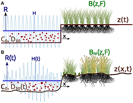
Figure 1. Schematic diagrams of the inputs of a 0-dimensional accretion model. (A) Simplified model with time-invariant maritime forcing (left) and uniform topography and vegetation (right). (B) Model with more realistic, time-dependent maritime forcing and variable topography and plant associations. R is the rate of sea level rise, C₀ is the suspended sediment concentration, D₅₀ is the median sediment grain size, H is the maximum tidal elevation for a given tidal cycle, B is the biomass of a given species, and F is the fitness function for that species.

We examine the effects of using observed rather than sinusoidal or predicted tidal forcing to simulate the vertical accretion on marsh platforms extracted from lidar topographic data. This approach is implemented in the model by describing the mineral accretion flux over a period Δt, Q_dep,Δt, as the sum of settling fluxes over each of the N_Δt tidal cycles in Δt (7).

$\begin{array}{ll}{Q}_{total,\Delta t}={\displaystyle \sum _{i=0}^{i=N_{\Delta t}}}{Q}_{dep,T_i}& (7)\end{array}$

We initially consider fixed values for C₀ and D₅₀, as detailed in section 2.3. Our aim is to determine whether these parameters can be used to explain observed marsh elevations and accretion rates, as well as the conditions necessary for platform elevations to match rising sea levels. Later in this contribution, we relax our assumptions about C₀ and D₅₀ and allow them to vary as free parameters.

2.3. Site Description and Sediment Supply Conditions

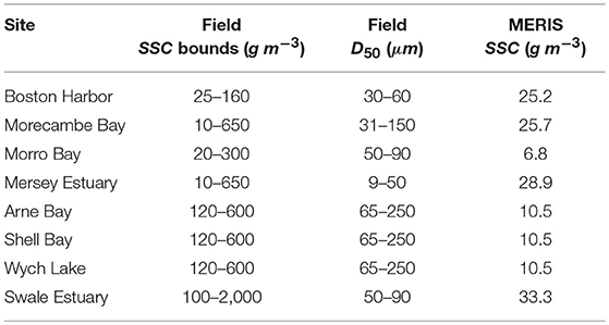
In this study, we examine 8 marsh sites where two lidar topographic surveys acquired at least 4 years apart are located in close proximity to a tidal gauge with a long-term record of hourly data. For each site, we obtain total suspended matter (TSM) using the GlobColour MERIS product (Barrot et al., 2007), which contains monthly values TSM in the Earth's oceans and lakes between 2002 and 2012. Monthly coverage of MERIS, however, is incomplete. Consequently, we use the averaged TSM between 2002 and 2012 in order to cover our sites. The angular resolution of MERIS products is 1/24° at the equator. While this is insufficient to observe the exact TSM value at our sites, MERIS data has already been used to calculate local sediment availability in global estimates of wetland response to sea level rise (Schuerch et al., 2018). In this study, we therefore use MERIS data in combination with field data on sediment supply conditions sourced from the literature, as described below. The location of each site is given in Figure 2 and the Supplementary Material.

FIGURE 2

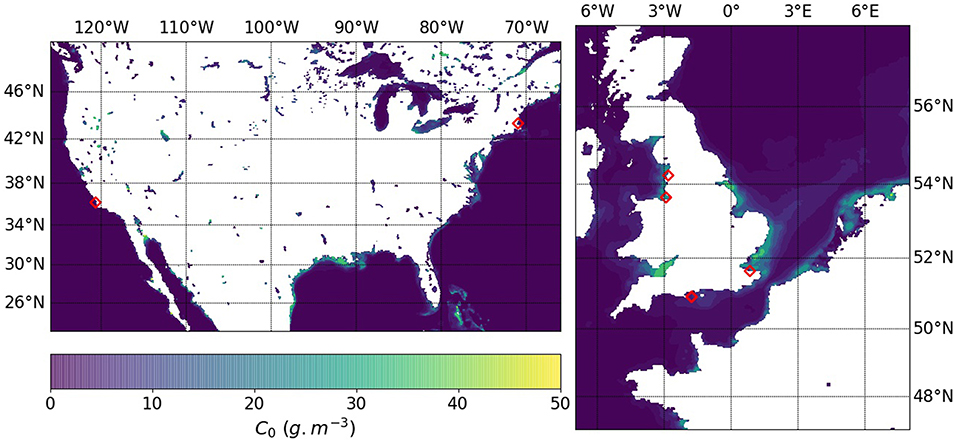
Figure 2. Location of the selected tidal stations over a map of averaged monthly Total Suspended Matter concentration between 2002 and 2012. In the United States, the stations are Port San Luis for the Morro Bay marsh (California) and Boston for the Boston Harbor marsh (Massachusetts). In the United Kingdom, the stations are: Heysham for the Morecambe Bay marsh, Gladstone for the Mersey Estuary marsh, Bournemouth for the Poole Harbour Shell Bay, Wych Lake and Arne Bay marshes, and Sheerness for the Swale Estuary marsh.

2.3.1. Boston Harbor

The marsh studied in Boston Harbor is located in Squantum, MA, and borders Quincy Bay, approximately 6 km from Boston Harbor tide gauge. Flume experiments conducted by Ravens and Gschwend (1999) show tidal flat sediments to range between 30 and 60μm in D₅₀, and to contain 3−4.5% of organic matter. Under stresses of 0.05 Pa, TSM oscillates around 25 g m⁻³, peaking around 160 g m⁻³ under stresses of 0.5 Pa. These values are slightly greater to those found by Hopkinson et al. (2018) in the nearby Plum Island Sound (median SSC around 15.6 g m⁻³ and peaks around 40 g m⁻³), however organic content is much lower than the 30% assumed in Plum Island.

2.3.2. Morro Bay

The marsh studied in Morro bay is located North of Morro Bay State Marine Reserve, CA, on the Chorro Creek estuary, approximately 20 km from Port San Luis tide gauge. Few data on sediment size, concentration and organic content was found for Morro Bay. Instead, we use data for San Francisco Bay, CA. There, acoustic backscatter was used to estimate sediment grain size between 50 and 90 μm and suspended solids to 20−300 g m⁻³ (Gartner, 2004).

2.3.3. Morecambe Bay

The marsh studied in Morecambe Bay is located South of Jenny's point, Lancashire, approximately 15 km from Heysham tide gauge. Few data were found for sediment concentrations. Instead we use data for the Mersey estuary. Aldridge (1997) finds sandy sediments around 150 μm and Pringle (1995) finds silts of around 31 μm. Gray and Scott (1977) mention loss on ignition of 8%.

2.3.4. Mersey Estuary

The marsh studied in the Mersey Estuary is located in Ellesmere Port, Cheshire, approximately 15 km from Gladstone tide gauge. Acoustic Doppler Current Profiler (ADCP) measurements in the Mersey river near Liverpool found D₅₀ in the channel to be approximately 9 μm, and were found up to approximately 50 μm. Suspended solids concentrations vary between 10 and 650 g m⁻³ (Holdaway et al., 1999).

2.3.5. Poole Harbour

The three marshes studied in the Poole Harbour, Dorset, are all under 7 km from the Bournemouth tide gauge. Gao and Collins (1994) show in the neighboring Christchurch Harbour that sediment grain sizes vary between 65 and 250 μm in the proximity of marshes, with concentrations measured around 120 g m⁻³ but known to reach 600 g m⁻³ during storm events (Green, 1940).

2.3.6. Sheerness

The marsh studied in the Swale Estuary, Kent, is approximately 16 km from the Sheerness tide gauge. Wharfe (1977) reports D₅₀ values ranging from 50 to 90 μm, while Zhou and Broodbank (2013) report concentrations ranging from 100 to 2, 000 g m⁻³.

2.4. Collection and Processing of Topographic Data

Topographic survey are sourced from either the NOAA Digital Coast archive or the United Kingdom Environment Agency. All datasets are referenced to their respective national topographic datum: the North American Vertical Datum 1988 in the USA and Ordnance Datum at Newlyn in the UK.

Errors in elevation measurements may stem from the georeferencing of the lidar point clouds. Vertical error margins are determined by comparing lidar elevations to the elevation of multiple ground control points. The root mean square error (RMSE) of this comparison is given by both data providers (Tables 1–3). Vegetation is another factor of error when measuring salt marsh ground elevation (Schmid et al., 2011; Parrish et al., 2014; Rogers et al., 2018). On Sapelo Island, GA, Hladik and Alber (2012) found that low plants such as short Spartina alterniflora and Batis maritima yielded positive errors of less than +0.05 m. Conversely, Chassereau et al. (2011) compared RTK-GPS and lidar elevations on Maddieanna Island, SC, a marsh dominated by Spartina alterniflora, with stem heights of 0.15–0.55 m on the platform and levees and up to 1.70 m on the lower marsh and creek banks. The study found positively skewed histograms of signed error, with the lowest positive errors (under +0.15 m) being far from creek banks, confirming the influence of stem height on the error in lidar elevation. To minimize the error due to vegetation, our selection of marshes excludes sites with dominant tall vegetation species (Table 1).

TABLE 1

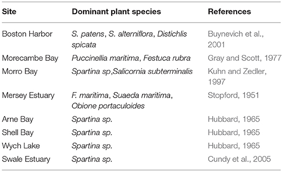
Table 1. Dominant plant species for the selected sites, sourced from literature on regional marsh systems and analog marshes.

TABLE 2

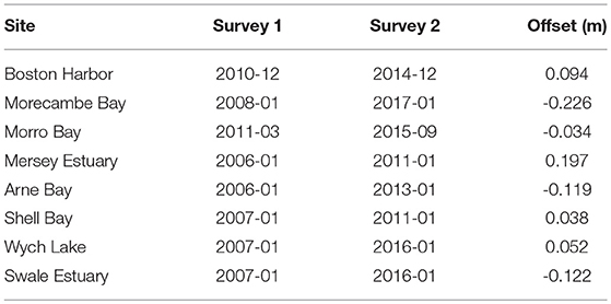
Table 2. Date of surveys and elevation offset for a stable structure between S2 and S1. Column 3 shows the offset in elevation between reference structures.

TABLE 3

Table 3. Sediment conditions used for the production of Figures 6, 7.

From the downloaded point clouds, we use CloudCompare (https://www.cloudcompare.org/) to generate rasters of minimum and maximum elevations within a grid cell, respectively, Z_min and Z_max. Grid cell size is determined to fit a minimum of 6 points per cell, up to a maximum of 3 m. The marsh platform elevation is then extracted from Z_min using the Topographic Identification of Platforms (TIP), which accurately delineates marsh platforms for grids of up to 3 m in horizontal resolution (Goodwin et al., 2018). For each survey, we select a low-relief, non-vegetated structure (road, car park, etc.) for which we calculate the 1st, 2nd and 3rd quartile of the difference Z_max − Z_min. Two subsampling methods are then applied to the marsh platform. First, pixels classified as marsh platforms for which Z_max − Z_min is less than the median of Z_max − Z_min of the reference structure are preserved, as shown for the Mersey Estuary in Figures 3A–C (red pixels). Similar figures for other sites are available in the Supplementary Material. This subsampling ensures that high elevation gradients do not exist within the pixel, whether they are due to topographic features (hummocks or pools) or locally high vegetation. Pixels classified as marsh platforms that are also levee points are selected by the second method (green pixels). Due to the larger spread of elevation and the potentially large errors in elevation associated with levee pixels, we do not use them further in this study (Figure 3D).

FIGURE 3

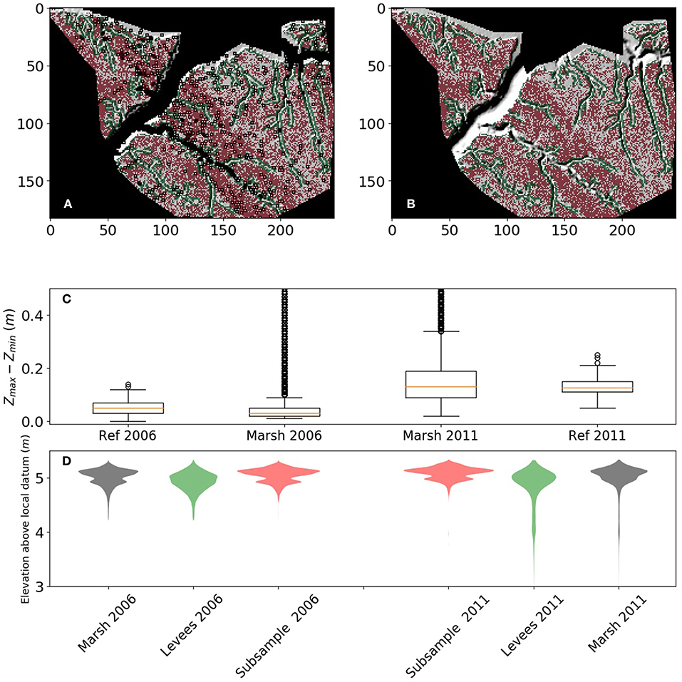
Figure 3. Marsh platform subsampling results for the Mersey Estuary Marsh. (A,B) Show the marsh hillshade (respectively for S1 and S2) overlayed with subsampled pixels (red) and levee pixels (green). (C) Boxplot of differences Z_max − Z_min for the reference infrastructure and the marsh platform. (D) Probability distribution functions for the entire marsh platform (gray), levee pixels (green), and subsample pixels (red).

Vertical offset between the two selected surveys is accounted for as the average difference of Z_min for the reference structure, the first survey being taken as reference by default. The values of vertical offset are given in Table 2.

2.5. Collection and Processing of Sea Level Data

Each selected marsh site is associated with a tidal station in its close vicinity. For these stations, we download sea level observations from the GESLA-2 dataset, a global collection of hourly sea level data up to the year 2015 (Woodworth et al., 2016), or the British Oceanographic Data Centre (BODC) data repository. From these records we extract the monthly mean high and low tides MHT_m and MLT_m. We fit a linear trend to each of these times series, the difference of which constitutes the mean tidal range MTR. The same process is applied to determine the trend of monthly observed highest high tide OHHT. Time series of monthly mean sea levels (MSL_m) were collected from the NOAA sea level trend dataset. For stations in the United Kingdom that do not have a long-term record of MSL_m, we choose the closest long-term tide gauge as a substitute. From this record we extract the linear trend of MSL_m, named MSL, the slope of which constitutes the rate of relative sea level rise RSLR. Figure 4a shows the tidal records with their associated metrics, as well as the 1-year subset of data used to calculate yearly deposition fluxes (see section 3). Figure 4b shows the cumulative distribution function of flooding time at each station, for both the whole record and the selected subset.

FIGURE 4

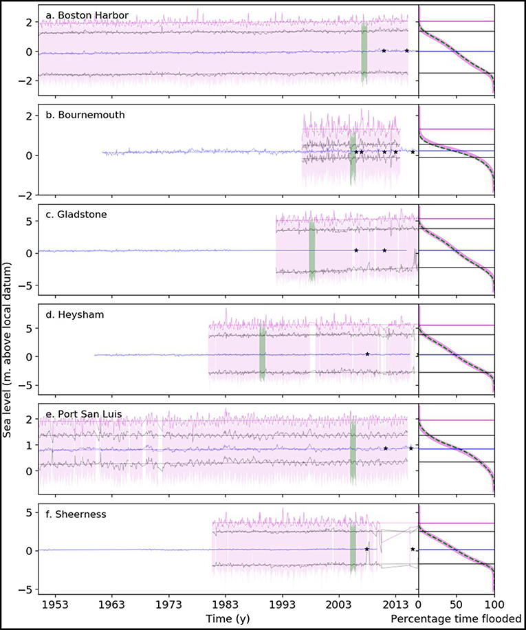
Figure 4. left: Hourly sea level record (pink) and monthly Mean Sea Level MSL (blue) for each station between 1950 and 2017. Black lines are, respectively, the monthly Mean High Tide MHT and Mean Low TIde MLT. Thicker pink lines are monthly Observed Highest High Tide OHHT. Straight lines are monthly linear trends for each metric. Green areas represent the most recent complete year of record. Right: Cumulative distribution function of flooded time for a given elevation for the whole tidal record (pink), and for the chosen representative year (dashed green). Horizontal lines are the most recent value of the linear monthly trends. (a–f) Tide gauges neighboring the examined marshes. Black stars indicate the dates of lidar surveys.

3. Results and Discussion

3.1. High Platform Elevations Cannot Be Explained by Sinusoidal Tidal Forcing

For each of the 8 selected marshes, Figure 5 shows the probability distribution function of elevation f_z of the marsh platform at the dates S1 (left of bar) and S2 (right of bar). Gray filled areas f_z represent the subsampled marsh platform (see Figure 3C). Gray lines represent the same pixel sets plus or minus half the RMSE reported by ground truthing reports. For each survey, marsh elevation is relative to its contemporary sea level. In all of the sites, irrespective of measurement error, the major part of the marsh platform lies within the upper tidal frame, defined as the range of elevations between MHT and OHHT. While megatidal marshes show a wider distribution, no platform occupies more than half of the upper tidal frame. This observation is supported by surveys of vegetation populations relative to tidal levels (Belliard et al., 2017) and refines the approach of Schuerch et al. (2018), where marshes are assumed to occupy the entire range of elevations between MSL and MHT.

FIGURE 5

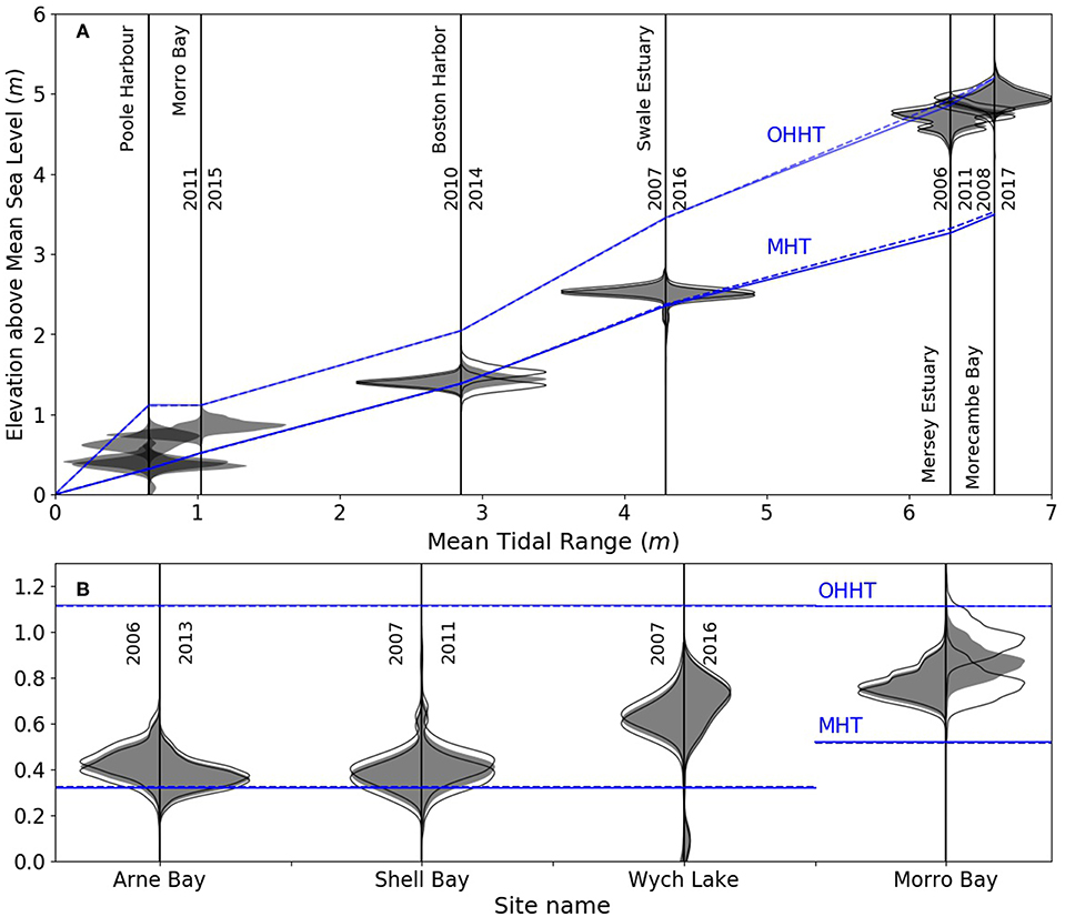
Figure 5. Probability distribution functions of marsh platform elevations relative to MSL for each examined marsh at the dates S1 (left - gray fill) and S2 (right - gray fill); Black lines indicate the possible vertical offset of the probability distribution functions due to lidar vertical error; Blue lines show the monthly trend for MHT and OHHT a the dates S1 (full) and S2 (dashed); (A) Marsh sites organized by Mean Tidal Range. (B) Detail of micro-tidal sites.

In models using a sinusoidal tidal forcing of amplitude H = MHT−MSL, the equilibrium elevation z_eq relative to MSL is given by Equation (8) (D'Alpaos et al., 2011):

$\begin{array}{ll}{z}_{eq}=H·(1-\frac{R}{k})& (8)\end{array}$

where k = Q_dep,y + Q_org,y [mm yr⁻¹] is the sum of yearly deposition and below-ground production rates. While z_eq is seldom truly reached, it gives an indication of the elevation toward which marsh platforms converge. Equation (8) suggests that, under sinusoidal forcing, no part of any marsh platform may reach elevations higher than MHT. This constraint is relaxed by the fact that platform elevation tends to lag behind sea level variations (Kirwan and Temmerman, 2009): salt marshes that have experienced higher sea levels may then be found at higher elevations.

All of the marshes examined in this study are higher than both their equilibrium elevations and their maximum elevation H + MSL. However, no stations other than Gladstone and Heysham have experienced late quaternary uplift (Shennan and Horton, 2002; Donnelly, 2006; Bromirski et al., 2011; Shennan et al., 2012) and no stations show significant negative modern variations in monthly MSL (see Figure 4). Hence, the high elevation of the examined marsh platforms cannot be explained by a sinusoidal forcing of amplitude H, notwithstanding the use of this forcing by several studies on marsh elevation change for lower marshes (e.g., Morris et al., 2002; Marani et al., 2007; D'Alpaos et al., 2011; Tambroni and Seminara, 2012; Da Lio et al., 2013).

Furthermore, platforms that are higher than z_eq are predicted by Equation (8) to lose elevation, as they are not flooded frequently enough to allow accretion rates that match sea level rise. However, Figure 5 shows that in all but two sites, platforms are gaining elevation on MSL. This affirmation stands for all but when extreme positive error in S1 and extreme negative error in S2 are considered. All the examined platforms therefore experience deposition, and may be considered active, rather than relics of higher sea levels. This result strongly suggests that the marsh platforms in our study depend on deposition of concentrated coarse sediment to maintain their position in the tidal frame, typically provided by spring tides and storms. The latter are shown by Castagno et al. (2018) to positively influence sediment import into back-barrier bays. This effect, however, is less important for fine sands (D₅₀ ≥ 125 μm), which hints at a potential depletion in this size fraction, which may in turn lead to marshes failing to keep pace with RSLR. Dependance on infrequent deposition events is also consistent with the findings of Mariotti et al. (2010) in micro-tidal back-barrier marshes, who showed that storm surges contribute to the erosion of scarps as well as to the recycling of eroded marsh sediment onto the platform.

3.2. Modeling Accretion Rates With Real Tidal Forcing Highlights the Influence of Elevation, Grain Size and Concentration

Following the observations of section 3.1, we examine the effect of using a realistic tidal forcing by simulating deposition fluxes over a year for each marsh site. The sea level record used to force accretion is a subset of the full tidal record for each station, shown as the green highlighted data in Figure 4. In this experiment, we use three sets of values for C₀ and D₅₀. Lower values for C₀ and D₅₀ referenced in Section 2.3 are the first set. The second set is D₅₀ = 50 μm, which is within the higher range of values used in long-term modeling studies (Marani et al., 2007; D'Alpaos et al., 2011). C₀ is determined by the values obtained from the MERIS Total Suspended Sediment (TSM) dataset at the location of the tidal station. In the third set, higher values for C₀ and D₅₀ referenced in section 2.3 are selected. Table 3 summarizes sediment supply conditions used in the simulations.

Figure 6 compares the observed and modeled elevation change of the dominant platform elevation z_max(fZ) relative to the terrestrial datum, with relative sea level rise as a reference. Despite the precautions taken to reduce error in the elevation samples, observed accretion rates (red bars) are visibly unreliable. For instance, Arne Bay exhibits negative accretion rates while Wych Lake and Shell Bay, located less than 5 km away, exhibit accretion rates close to those recorded at Wax Lake Delta, one of the fastest accreting marshes in the world. Morro Bay and Boston Harbor also exhibit unrealistic accretion rates, particularly in regard to the low rates of associated sea level rise. While such rapid elevation variations have been observed using SETs (Kirwan et al., 2016), they may also be the product of uncertainty in elevation values. Indeed, errors in the measurement of elevation for both S1 and S2 lead to considerable error in rates of accretion, as shown by the error bars in Figure 6.

FIGURE 6

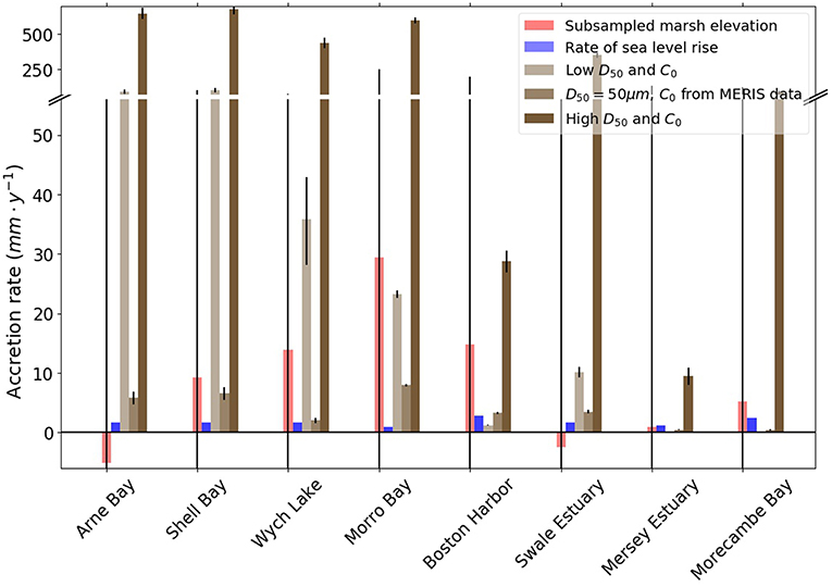
Figure 6. Magnitude of deposition rates (red and brown bars), with relative sea level rise RSLR for reference, for each site; the initial elevation is the normalized dominant elevation of the platform z_max(fZ). Black lines indicate vertical error.

However, the elevation error in S1 typically leads to errors of 5% or less on the modeled accretion rate (brown bars). Although variations in sediment supply and flooding patterns prevent a direct comparison between sites, we observe an overall decrease in modeled deposition rates with increasing tidal range and platform elevation. Conversely, we note a significant positive response of accretion rates to the combined increase in sediment size and concentration, as shown by the differences in accretion rates between low C₀ and D₅₀ and high C₀ and D₅₀. This response leads us to postulate that the low values of C₀ are the cause for the low modeled accretion rates when using MERIS data. Indeed, the MERIS dataset has a spatial resolution of 300 m and is primarily an oceanic dataset. It does not account for complex coastal inlets, estuaries and bays where salt marshes are found, and where higher concentrations are likely to be found (Amos and Alfoldi, 1979). Furthermore, Fagherazzi et al. (2014) find strong spatial variations in sediment size within the tidal creeks of a single site at Plum Island Sound. In this respect, the site-specific data collected in section 2.3 is likely representative of the spatial variability of sediment supply found in the sites examined. The relative influence of C₀ and D₅₀, however, is not discernable at this point.

3.3. Constraints on Sediment Supply and Consequences for Platform Equilibrium

Whether a marsh keeps pace with sea levels has been suggested to depend on forcing sediment concentration (Kirwan et al., 2010; D'Alpaos et al., 2011; Kirwan and Megonigal, 2013). We establish in Section 3.2 that deposition is also conditioned by the initial platform elevation, as suggested by Cahoon and Reed (1995), and the grain size of the deposited sediment. We calculate Q_dep for a range of C₀ and D₅₀, assuming a contribution of 6% from below-ground production Q_org. This value is the lower bound of a range estimated from loss on ignition organic matter contents for several marshes around the world (Crooks et al., 2002; Neubauer, 2008; Roner et al., 2016), and approximates to local data in Boston Harbor and Morro Bay (see section 2.3). For each site, Figure 7 shows the contour lines of C₀ and D₅₀ values that yield given values of k = Q_dep+Q_org. The dashed blue line corresponds to conditions on C₀ and D₅₀ for marsh accretion to match the current RSLR. Dashed red lines indicate the observed accretion rates, but do not represent the associated error. Sediment supply conditions corresponding to low and high C₀ and D₅₀ bound the gray box, and the black star represents the concentration determined using the MERIS data and D₅₀ = 50 μm. We remind the reader that due to the assumption of negligible turbulence on the marsh surface, Q_dep is likely overestimated and therefore the required sediment supply to match a given RSLR is likely under estimated.

FIGURE 7

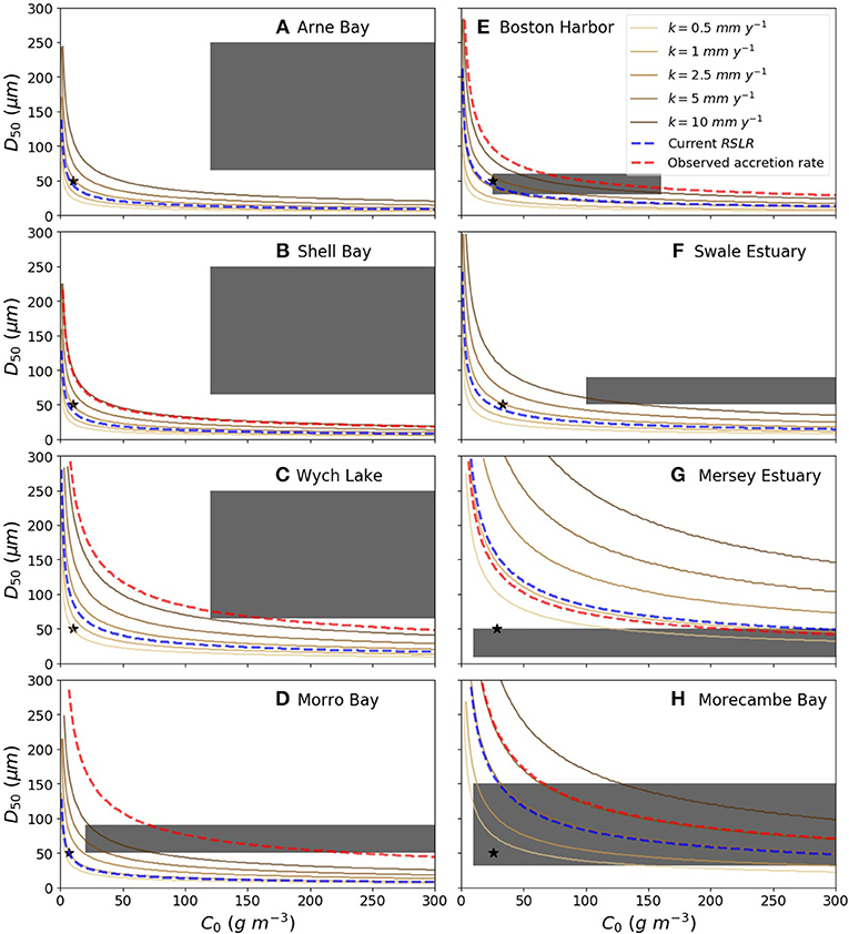
Figure 7. Contour lines representing conditions on C₀ and D₅₀ for total accretion k = Q_dep + Q_org to reach the indicated values. Here, Q_org = 0.06 · Q_dep; Gray boxes bound sediment supply conditions from low C₀ and D₅₀ to high C₀ and D₅₀. Black stars represent C₀ conditions obtained from MERIS data, with D₅₀ = 50 μm. Blue dashed lines represent the conditions required to match RSLR, and red dashed lines the conditions to match observed accretion rates. (A–H) Marsh sites examined, ordered by Mean Tidal Range.

In all cases, the contours follow a hyperbolic curve. This behavior implies that at high sediment concentrations, variations in C₀ have less impact on Q_dep than variations in D₅₀, and vice versa. Conversely, the point of the contour line that is closest to graph origin represents the conditions where variations in each parameters exert an equal influence on accretion rates. This behavior is preserved along the 1:1 diagonal. High sediment concentrations require high shear stress at the bed to mobilize sediment (Fagherazzi et al., 2006) if generated in situ. If the sediment is sourced from either offshore or rivers, high turbulence is needed to keep sediment in suspension. High suspended sediment concentrations are associated with strong currents or high waves, increasingly so for large particle sizes (Yang et al., 2008). Consequently, we may expect higher sediment concentrations to be associated with larger particle sizes. Such conditions are typical of storm events, spring tides or fluvial flood discharges. They may be observed on the field, for instance when gravel is backed-up against marsh scarps after storm events, or when strong tides leave sandy trail bars on the lee side of pioneer plants.

Figures 7A–C represent three neighboring marshes in Poole Harbour, Dorset, UK, for which tidal and sediment conditions are considered identical. Wych Lake (Figure 7C) is higher in the tidal frame than the other sites, and as a consequence, the contour lines are both further from the origin and further apart. Hence, for equal sediment supplies and tidal forcing, increasing elevation reduces deposition rates and increases the demand in sediment to maintain elevation within the tidal frame. For example, platforms in Morecambe Bay and the Mersey Estuary (Figures 7G–H) are close to OHHT, and are seldom flooded. As a consequence, not only do these sites require more sediment to match current rates of sea level rise, but they would also require a greater increase in C₀ or D₅₀ if RSLR increased. This situation is hinted at by Pringle (1995), who finds medium to coarse silts (31 μm) and very fine sands of up to 100 μm in Morecambe Bay marshes. Conversely, ranges of 20 − 40 μm were observed by Roner et al. (2016) in the Venice Lagoon, where salt marshes are notoriously low in the tidal frame (Da Lio et al., 2013).

We show the conditions necessary to match observed positive accretion rates (dashed red lines), but recommend caution when considering these data (see section 3.2). Indeed, though it seems that most sediment supply condition boxes (gray boxes) contain the dashed red lines, the existence of negative accretion when conditions predict more than 10 mm y⁻¹ of accretion demands a critical view of the observed accretion values. Regardless, all field-measured sediment supply conditions generate enough accretion in all sites, except the Mersey Estuary and Morecambe Bay (Figures 7G–H), for the platform to keep up with current RSLR (dashed blue lines). Aside from Boston Harbour (Figure 7E), even the lower bounds of measured sediment supply are sufficient to match more than 10 mm y⁻¹ of sea level rise. Our application of Stokes' law with negligible current and turbulence may explain this overestimation of k. However, we must also consider that field measurements provide only a snapshot of sediment supply conditions at any given location.

Leroux (2013) highlighted the high temporal variability of sediment supply; he measured peak concentrations of up to 5, 000 g m⁻³ during a spring tide, while base concentrations were 500 g m⁻³ in tidal creeks of the Mont-Saint-Michel Bay, France. The high shear stresses caused by storms also generate peaks in sediment concentrations (Fagherazzi and Priestas, 2010). In this respect, averaged MERIS data (black stars) may better represent the temporal variability of sediment supply. To further improve our understanding of sediment supply, we suggest that k contour lines may be combined with accretion monitoring through marker horizons and grain size distribution (GSD) analyses to determine average sediment concentrations during deposition events. While our 0-D model does not account for distance to creeks, the results of Zhang et al. (2019) show that it is an important factor of marsh deposition, and we suggest that these results should orient future methods of deposition measures.

3.4. Insight on the Roles of Elevation and Tidal Range

In this section, we compare the 8 marsh sites to better understand the interaction between platform elevation and tidal records. In Figure 8, we calculate k for the same range of sediment supply conditions as in section 3.3 and represent the conditions leading to k = 2.5 mm y⁻¹. Each subplot shows the accretion contour lines for each site for various initial elevations z₀. Indeed, elevation within the tidal frame determines the (1) proportion of N_Δt tidal cycles for which the platform floods (Equation 6), and (2) the maximum depth D_max of each flooding event, thus influencing deposition within each cycle (Equation 7). Although below-ground production is known to vary with elevation, these variations are not well quantified above elevations of MHT (Morris et al., 2002), and we therefore maintain Q_org = 0.06·Q_dep.

FIGURE 8

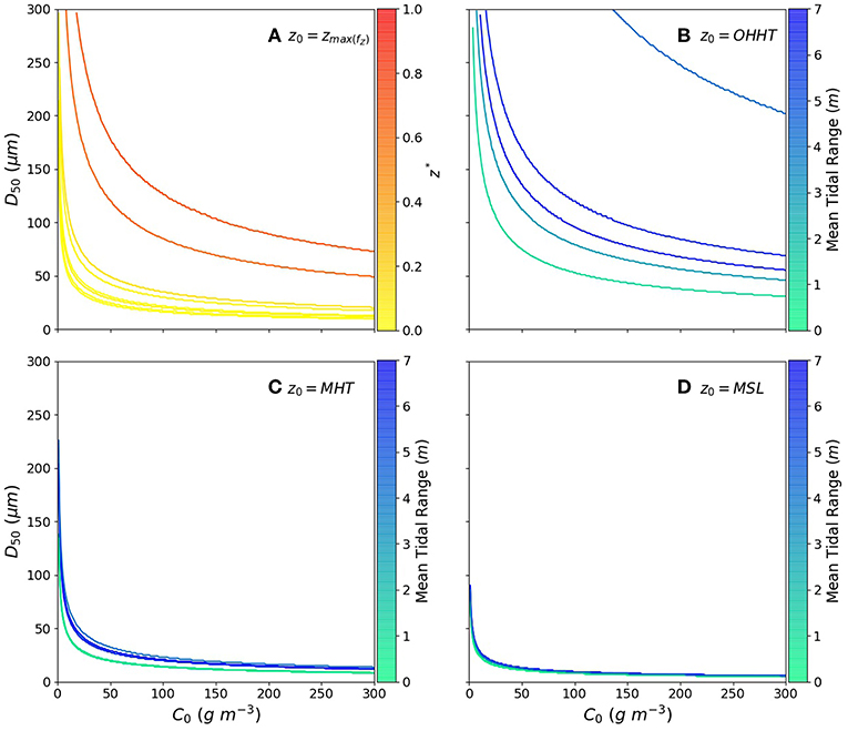
Figure 8. Necessary values of C₀ and D₅₀ for total accretion to reach k = 2.5 mm y⁻¹; (A) initial elevation z₀ = z_max(fZ), colored by increasing z*. (B) z₀ = OHHT. (C) z₀ = MHT. (D) z₀ = MSL; the last three subplots are colored by mean tidal range.

In Figure 8A, the initial elevation is the observed main platform elevation z_max(fZ). Regardless of mean tidal range, the normalized elevation in the upper tidal frame, defined as z* in Equation (9), exerts a positive influence on the sediment supply necessary to meet k = 2.5 mm y⁻¹.

$\begin{array}{ll}{z}^{*}=\frac{z-MHT}{OHHT-MHT}& (9)\end{array}$

We note that for z₀ = OHHT (Figure 8B), sediment requirements are so high that for Boston Harbor and the Swale Estuary, sediment larger than fine sand would be needed for marshes to be at equilibrium of moderate sea level rise rates. Such conditions are typical of beaches and sand dunes rather than marshes (Hayden et al., 1995), suggesting that flooding patterns at these sites do not allow marshes to reach these elevations.

Conversely, if z₀ = MHT, very little variation between sites of different tidal ranges is observed, suggesting that the effect of tidal range on accretion rates increases with platform elevation. Hence, similar sediment supply conditions shown (Figure 8C) may allow low marsh platforms around the world to withstand moderate sea level rise rates of RSLR = 2.5 mm y⁻¹, whereas local tidal regimes would affect high platforms more strongly. This low sediment demand is similar to that observed in Figure 8D, where initial elevations are z₀ = MSL. For these low elevations, mean tidal range also exerts a weak influence on accretion rates. More importantly, the little difference in accretion rates between z₀ = MSL and z₀ = MHT imply that pioneer platforms are likely to reach MHT, thus ensuring the regeneration of marsh surface area after lateral erosion events. We note that our model does not account for variable sediment concentrations on the platform, and is likely to overestimate deposition on parts of the platform that are far from creeks or scarps. Indeed, Temmerman et al. (2005) show that deposition rates decrease with distance from creeks and marsh edges. Pioneer platforms with different creek network properties, due for example to vegetation development (Kearney and Fagherazzi, 2016), may grow at different rates.

4. Conclusions

In this contribution, we test a 0-dimensional settling model to estimate elevation change on real salt marsh platforms, and compare these results with accretion fluxes derived from DEM surveys taken at least four years apart. While elevation changes observed through lidar have too high errors to yield accurate results, initial elevation measurements are sufficiently accurate to examine model results and their sensitivity to sediment supply conditions. We find that using a sinusoidal tidal forcing to simulate elevation evolution cannot explain the current elevation of the marshes we examined, which were located between MHT and OHHT. While we did not examine enough sites to draw general conclusions on the distribution of salt marsh platforms within the tidal frame, our results suggest that simplified sinusoidal tides cannot account for the full evolution of salt marshes.

Using a representative subset of real tidal forcing, we calculate settling fluxes that better explain current platform elevations. When accounting for a 6% contribution of belowground organic production to accretion fluxes, modeled accretion rates for marshes that are low in the upper tidal frame (but still above MHT) are mostly sufficient to keep pace with current rates of relative sea level rise under most observed sediment supply conditions determined by MERIS. Conversely, sites that are closer to OHHT require coarser or more concentrated sediment. The low hydroperiod associated with such high platforms suggests that small or light flocs do not have time to settle in sufficient quantity for the platform to maintain its elevation. Under storm surge conditions, however, advection of highly concentrated fine material and prolonged hydroperiod may counteract the effect of elevation.

It follows that marshes that reach a high position in tidal frame should contain coarser sediment than platforms that do not attain this elevation, unless they are subject to frequent storms. The existence of such high platforms is therefore conditioned by the availability of coarse sediment or finer material in high volumes (or very high organic matter contents), typically mobilized during storms, floods and spring tides. Conversely, we find that low platforms require a weaker sediment supply conditions to keep pace with RSLR. Further investigation into accretion rates with low starting elevations (MHT and MSL) suggests that established low platforms are likely to contribute to long-term marsh regeneration regardless of tidal regimes, but also that plant establishment is likely the bottleneck of marsh progradation processes.

To add weight to the conclusions drawn above, further research may investigate the relationship between marsh elevation and tidal records over a larger dataset. Furthermore, measuring sedimentation and back-calculating sediment concentration from field samples in different sites would allow to confirm the behavior suggested by the model. Future work may also investigate the size of deposited particles at various distances from scarps and tidal creeks to determine the detailed mechanisms of settling on wide vegetated platforms.

Author Contributions

GG designed the study, collected and analyzed the data and wrote the article with input in all aspects from SM.

Funding

GG is funded by the Natural Environment Research Council Doctoral Training Partnership grant NERC NE/L002558/1. SM was supported by the Leverhulme Foundation (IAF-2014-009).

Conflict of Interest Statement

The authors declare that the research was conducted in the absence of any commercial or financial relationships that could be construed as a potential conflict of interest.

Acknowledgments

The authors wish to acknowledge Dimitri Lague for his guidance on the use of the CloudCompare command line, and on the analysis of point clouds in general. the authors also thank the Geomatics Department at the Department for Environment, Food and Rural Affairs.

Supplementary Material

The Supplementary Material for this article can be found online at: https://www.frontiersin.org/articles/10.3389/fenvs.2019.00062/full#supplementary-material

References

Aldridge, J. N. (1997). Hydrodynamic model predictions of tidal asymmetry morecambe bay. Estuar. Coast. Shelf Sci. 44, 39–56. doi: 10.1006/ecss.1996.0113

CrossRef Full Text | Google Scholar

Amos, C. L., and Alfoldi, T. T. (1979). The determination of suspended sediment concentration in a macrotidal system using landsat data. J. Sediment. Petrol. 49, 159–174. doi: 10.1306/212F76DF-2B24-11D7-8648000102C1865D

CrossRef Full Text | Google Scholar

Anisfeld, S. C., Hill, T. D., and Cahoon, D. R. (2016). Elevation dynamics in a restored versus a submerging salt marsh in Long Island Sound. Estuar. Coast. Shelf Sci. 170, 145–154. doi: 10.1016/j.ecss.2016.01.017

CrossRef Full Text | Google Scholar

Barrot, G., Mangin, A., and Pinnock, S. (2007). GlobColour Global Ocean Colour for Carbon Cycle Research Product User Guide. Technical report.

Google Scholar

Belliard, J. P., Di Marco, N., Carniello, L., and Toffolon, M. (2016). Sediment and vegetation spatial dynamics facing sea-level rise in microtidal salt marshes: insights from an ecogeomorphic model. Adv. Water Resour. 93, 249–264. doi: 10.1016/j.advwatres.2015.11.020

CrossRef Full Text | Google Scholar

Belliard, J. P., Temmerman, S., and Toffolon, M. (2017). Ecogeomorphic relations between marsh surface elevation and vegetation properties in a temperate multi-species salt marsh. Earth Surf. Process. Landf. 42, 855–865. doi: 10.1002/esp.4041

CrossRef Full Text | Google Scholar

Bromirski, P. D., Miller, A. J., Flick, R. E., and Auad, G. (2011). Dynamical suppression of sea level rise along the Pacific coast of North America: indications for imminent acceleration. J. Geophys. Res. Oceans 116, 1–13. doi: 10.1029/2010JC006759

CrossRef Full Text | Google Scholar

Buynevich, I. V., Fitzgerald, D. M., Smith, L. B. J., and Doughertyt, A. J. (2001). Stratigraphic evidence for historical position of the East Cambridge Shoreline , Boston. J. Coast. Res. 3, 15–20. Available online at: https://www.jstor.org/stable/4300213

Google Scholar

Cahoon, D. R. (2015). Estimating relative sea-level rise and submergence potential at a coastal wetland. Estuar. Coasts 38, 1077–1084. doi: 10.1007/s12237-014-9872-8

CrossRef Full Text | Google Scholar

Cahoon, D. R., and Reed, D. J. (1995). Relationships among marsh surface topography, hydroperiod, and soil accretion in a deteriorating louisiana salt marsh. J. Coast. Res. 11, 357–369.

Google Scholar

Carniello, L., Defina, A., Fagherazzi, S., and D'Alpaos, L. (2005). A combined wind wave-tidal model for the Venice lagoon, Italy. J. Geophys. Res. 110, 1–15. doi: 10.1029/2004JF000232

CrossRef Full Text | Google Scholar

Castagno, K. A., Jiménez-robles, A. M., and Donnelly, J. P. (2018). Intense storms increase the stability of tidal bays. Geophys. Res. Lett. 45, 5491–5500. doi: 10.1029/2018GL078208

CrossRef Full Text | Google Scholar

Chassereau, J. E., Bell, J. M., and Torres, R. (2011). A comparison of GPS and lidar salt marsh DEMs. Earth Surf. Process. Landf. 36, 1770–1775. doi: 10.1002/esp.2199

CrossRef Full Text | Google Scholar

Crooks, S., Schutten, J., Sheern, G. D., Pye, K., and Davy, A. J. (2002). Drainage and elevation as factors in the restoration of salt marsh in Britain. Restorat. Ecol. 10, 591–602. doi: 10.1046/j.1526-100X.2002.t01-1-02036.x

CrossRef Full Text | Google Scholar

Crosby, S. C., Sax, D. F., Palmer, M. E., Booth, H. S., Deegan, L. A., and Bertness, M. D., et al. (2016). Salt marsh persistence is threatened by predicted sea-level rise. Estuar. Coast. Shelf Sci. 181, 93–99. doi: 10.1016/j.ecss.2016.08.018

CrossRef Full Text | Google Scholar

Cundy, A. B., Hopkinson, L., Lafite, R., Spencer, K., Taylor, J. A., and Ouddane, B., et al. (2005). Heavy metal distribution and accumulation in two Spartina sp. -dominated macrotidal salt marshes from the Seine estuary (France) and the Medway estuary (UK). Appl. Geochem. 20, 1195–1208. doi: 10.1016/j.apgeochem.2005.01.010

CrossRef Full Text | Google Scholar

Da Lio, C., D'Alpaos, A., and Marani, M. (2013). The secret gardener: vegetation and the emergence of biogeomorphic patterns in tidal environments. Philos. Trans. Ser. A Math. Phys. Eng. Sci. 371:20120367. doi: 10.1098/rsta.2012.0367

CrossRef Full Text | Google Scholar

D'Alpaos, A., Lanzoni, S., Marani, M., Fagherazzi, S., and Rinaldo, A. (2005). Tidal network ontogeny: channel initiation and early development. J. Geophys. Res. 110, 1–14. doi: 10.1029/2004JF000182

CrossRef Full Text | Google Scholar

D'Alpaos, A., Lanzoni, S., Marani, M., and Rinaldo, A. (2007). Landscape evolution in tidal embayments: modeling the interplay of erosion, sedimentation, and vegetation dynamics. J. Geophys. Res. 112, 1–17. doi: 10.1029/2006JF000537

CrossRef Full Text | Google Scholar

D'Alpaos, A., Mudd, S. M., and Carniello, L. (2011). Dynamic response of marshes to perturbations in suspended sediment concentrations and rates of relative sea level rise, J. Geophys. Res. 116:F04020. doi: 10.1029/2011JF002093

CrossRef Full Text | Google Scholar

Donnelly, J. P. (2006). A revised late holocene sea-level record for Northern Massachusetts, USA. J. Coast. Res. 225, 1051–1061. doi: 10.2112/04-0207.1

CrossRef Full Text | Google Scholar

Fagherazzi, S., Carniello, L., D'Alpaos, L., and Defina, A. (2006). Critical bifurcation of shallow microtidal landforms in tidal flats and salt marshes. Proc. Natl. Acad. Sci. U.S.A. 103, 8337–8341. doi: 10.1073/pnas.0508379103

PubMed Abstract | CrossRef Full Text | Google Scholar

Fagherazzi, S., Kirwan, M. L., Mudd, S. M., Guntenspergen, G. R., Temmerman, S., and Rybczyk, J. M., et al. (2012). Numerical models of salt marsh evolution: ecological, geormorphic, and climatic factors. Rev. Geophys. 50, 1–28. doi: 10.1029/2011RG000359

CrossRef Full Text | Google Scholar

Fagherazzi, S., Mariotti, G., Banks, A. T., Morgan, E. J., and Fulweiler, R. W. (2014). The relationships among hydrodynamics, sediment distribution, and chlorophyll in a mesotidal estuary. Estuar. Coast. Shelf Sci. 144, 54–64. doi: 10.1016/j.ecss.2014.04.003

CrossRef Full Text | Google Scholar

Fagherazzi, S., and Priestas, A. M. (2010). Sediments and water fl uxes in a muddy coastline: interplay between waves and tidal channel hydrodynamics. Earth Surf. Process. Landf. 293, 284–293. doi: 10.1002/esp.1909

CrossRef Full Text | Google Scholar

Gao, A. S., and Collins, M. B. (1994). Analysis of grain size trends, for defining sediment transport pathways in marine environments. J. Coast. Res. 10, 70–78.

Google Scholar

Gartner, J. W. (2004). Estimating suspended solids concentrations from backscatter intensity measured by acoustic Doppler current profiler in San Francisco Bay, California. Mar. Geol. 211, 169–187. doi: 10.1016/j.margeo.2004.07.001

CrossRef Full Text | Google Scholar

Goodwin, G. C., Mudd, S. M., and Clubb, F. J. (2018). Unsupervised detection of salt marsh platforms: a topographic method. Earth Surf. Dyn. 6, 239–255. doi: 10.5194/esurf-6-239-2018

CrossRef Full Text | Google Scholar

Gray, A. J., and Scott, R. (1977). The ecology of morecambe bay. VII. The distribution of Puccinellia maritima, Festuca rubra and Agrostis stolonifera in the Salt Marshes. Brit. Ecol. Soc. 14, 229–241. doi: 10.2307/2401838

CrossRef Full Text | Google Scholar

Green, F. H. W. (1940). Poole Harbour - a hydrographic survey 1938-9. Geograph. Publ.

Hayden, B. P., Santos, M. C. F. V., Shao, G., and Kochel, R. C. (1995). Geomorphological controls on coastal vegetation at the virginia Coast Reserve. Geomorphology 13, 283–300. doi: 10.1016/0169-555X(95)00032-Z

CrossRef Full Text | Google Scholar

Hladik, C., and Alber, M. (2012). Accuracy assessment and correction of a LIDAR-derived salt marsh digital elevation model. Remote Sens. Environ. 121, 224–235. doi: 10.1016/j.rse.2012.01.018

CrossRef Full Text | Google Scholar

Holdaway, G. P., Thorne, P. D., Flatt, D., Jones, S. E., and Prandle, D. (1999). Comparison between ADCP and transmissometer measurements of suspended sediment concentration. Continent. Shelf Res. 19, 421–441. doi: 10.1016/S0278-4343(98)00097-1

CrossRef Full Text | Google Scholar

Hopkinson, C., Morris, J. T., Fagherazzi, S., Wollheim, W. M., and Raymond, P. A. (2018). Lateral marsh edge erosion as a source of sediments for vertical marsh accretion. J. Geophys. Res. G 123, 2444–2465. doi: 10.1029/2017JG004358

CrossRef Full Text | Google Scholar

Hubbard, J. C. E. (1965). Spartina marshes in Southern England: VI. Pattern of invasion in poole harbour. Brit. Ecol. Soc. 53, 799–813. doi: 10.2307/2257637

CrossRef Full Text | Google Scholar

IPCC, I. P. o. C. C. (2014). Coastal systems and low-lying areas. Climate Change 2014: Impacts, Adaptation, and Vulnerability. Part A: Global and Sectoral Aspects. Contribution of Working Group II to the Fifth Assessment Report of the Intergovernmental Panel on Climate Change, 361–409.

Kearney, W. S., and Fagherazzi, S. (2016). Salt marsh vegetation promotes efficient tidal channel networks. Nat. Commun. 7, 1–7. doi: 10.1038/ncomms12287

PubMed Abstract | CrossRef Full Text | Google Scholar

Kennish, M. J. (2001). Coastal salt marsh systems in the U.S.: a review of anthropogenic impacts. J. Coast. Res. 17, 731–748. Available online at: https://www.jstor.org/stable/4300224

Google Scholar

Kirwan, M., and Temmerman, S. (2009). Coastal marsh response to historical and future sea-level acceleration. Quatern. Sci. Rev. 28, 1801–1808. doi: 10.1016/j.quascirev.2009.02.022

CrossRef Full Text | Google Scholar

Kirwan, M. L., Guntenspergen, G. R., D'Alpaos, A., Morris, J. T., Mudd, S. M., and Temmerman, S. (2010). Limits on the adaptability of coastal marshes to rising sea level. Geophys. Res. Lett. 37, 1–5. doi: 10.1029/2010GL045489

CrossRef Full Text | Google Scholar

Kirwan, M. L., and Megonigal, J. P. (2013). Tidal wetland stability in the face of human impacts and sea-level rise. Nature 504, 53–60. doi: 10.1038/nature12856

PubMed Abstract | CrossRef Full Text | Google Scholar

Kirwan, M. L., Murray, A. B., Donnelly, J. P., and Corbett, D. R. (2011). Rapid wetland expansion during European settlement and its implication for marsh survival under modern sediment delivery rates. Geology 39, 507–510. doi: 10.1130/G31789.1

CrossRef Full Text | Google Scholar

Kirwan, M. L., Temmerman, S., Skeehan, E. E., Guntenspergen, G. R., and Fagherazzi, S. (2016). Overestimation of marsh vulnerability to sea level rise. Nat. Clim. Change 6, 253–260. doi: 10.1038/nclimate2909

CrossRef Full Text | Google Scholar

Kuhn, N., and Zedler, J. B. (1997). Differential effects of salinity and soil saturation on native and exotic plants of a coastal salt marsh. Estuaries 20, 391–403. doi: 10.2307/1352352

CrossRef Full Text | Google Scholar

Lerberg, S. (2016). Assessing tidal marsh resilience to sea-level rise at broad geographic scales with multi-metric indices. Biol. Conserv. 204, 263–275. doi: 10.1016/j.biocon.2016.10.015

CrossRef Full Text | Google Scholar

Leroux, J. (2013). Chenaux tidaux et Dynamique des prés-salés en Régime méga-tidal: Approche Multi-Temporelle du Siècle à L'événement de Marée. Géomorphologie. Université Européenne de Bretagne, Université Rennes 1.

Google Scholar

Marani, M., Da Lio, C., and D'Alpaos, A. (2013). Vegetation engineers marsh morphology through multiple competing stable states. Proc. Natl. Acad. Sci. U.S.A. 110, 3259–3263. doi: 10.1073/pnas.1218327110

PubMed Abstract | CrossRef Full Text | Google Scholar

Marani, M., D'Alpaos, A., Lanzoni, S., Carniello, L., and Rinaldo, A. (2007). Biologically-controlled multiple equilibria of tidal landforms and the fate of the Venice lagoon. Geophys. Res. Lett. 34, 1–5. doi: 10.1029/2007GL030178

CrossRef Full Text | Google Scholar

Marani, M., D'Alpaos, A., Lanzoni, S., Carniello, L., and Rinaldo, A. (2010). The importance of being coupled: stable states and catastrophic shifts in tidal biomorphodynamics. J. Geophys. Res. 115, 1–15. doi: 10.1029/2009JF001600

CrossRef Full Text | Google Scholar

Mariotti, G., and Fagherazzi, S. (2010). A numerical model for the coupled long-term evolution of salt marshes and tidal flats. J. Geophys. Res. 115, 1–15. doi: 10.1029/2009JF001326

CrossRef Full Text | Google Scholar

Mariotti, G., Fagherazzi, S., Wiberg, P. L., McGlathery, K. J., Carniello, L., and Defina, A. (2010). Influence of storm surges and sea level on shallow tidal basin erosive processes. J. Geophys. Res. 115, 1–17. doi: 10.1029/2009JC005892

CrossRef Full Text | Google Scholar

Möller, I., Kudella, M., Rupprecht, F., Spencer, T., Paul, M., and van Wesenbeeck, B. K., et al. (2014). Wave attenuation over coastal salt marshes under storm surge conditions. Nat. Geosci. 7, 727–731. doi: 10.1038/ngeo2251

CrossRef Full Text | Google Scholar

Morris, J. T., Sundareshwar, P. V., Nietch, C. T., Kjerfve, B., and Cahoon, D. R. (2002). Responses of coastal wetlands to rising sea level. Ecology 83, 2869–2877. doi: 10.1890/0012-9658(2002)083[2869:ROCWTR]2.0.CO;2

CrossRef Full Text | Google Scholar

Mudd, S. M., D'Alpaos, A., and Morris, J. T. (2010). How does vegetation affect sedimentation on tidal marshes? Investigating particle capture and hydrodynamic controls on biologically mediated sedimentation, J. Geophys. Res. 115:F03029. doi: 10.1029/2009JF001566

CrossRef Full Text | Google Scholar

Nepf, H. M. (1999). Drag, turbulence, and diffusion in flow through emergent vegetation. Water Resour. Res. 35, 479–489. doi: 10.1029/1998WR900069

CrossRef Full Text | Google Scholar

Neubauer, S. C. (2008). Contributions of mineral and organic components to tidal freshwater marsh accretion. Estuar. Coast. Shelf Sci. 78, 78–88. doi: 10.1016/j.ecss.2007.11.011

CrossRef Full Text | Google Scholar

Nolte, S., Koppenaal, E. C., Esselink, P., Dijkema, K. S., Schuerch, M., and De Groot, A. V., et al. (2013). Measuring sedimentation in tidal marshes: a review on methods and their applicability in biogeomorphological studies. J. Coast. Conserv. 17, 301–325. doi: 10.1007/s11852-013-0238-3

CrossRef Full Text | Google Scholar

Parrish, C. E., Rogers, J. N., and Calder, B. R. (2014). Assessment of waveform features for lidar uncertainty modeling in a coastal salt marsh environment. IEEE Geosci. Remote Sens. Lett. 11, 569–573. doi: 10.1109/LGRS.2013.2280182

CrossRef Full Text | Google Scholar

Pennings, S. C., Selig, E. R., Houser, L. T., and Bertness, M. D. (2003). Geographic variation in positive and negative interactions among salt marsh plants. Ecology 84, 1527–1538. doi: 10.1890/0012-9658(2003)084[1527:GVIPAN]2.0.CO;2

CrossRef Full Text | Google Scholar

Pringle, A. W. (1995). Erosion of a cyclic saltmarsh in Morecambe Bay, North-West England. Earth Surf. Process. Landf. 20, 387–405. doi: 10.1002/esp.3290200502

CrossRef Full Text | Google Scholar

Ravens, T. M., and Gschwend, P. M. (1999). Flume measurements of sediment erodibility in boston harbor. J. Hydraulic Eng. 125, 998–1005. doi: 10.1061/(ASCE)0733-9429(1999)125:10(998)

CrossRef Full Text | Google Scholar

Rogers, J. N., Parrish, C. E., Ward, L. G., and Burdick, D. M. (2016). Assessment of elevation uncertainty in salt marsh environments using discrete-return and full-waveform lidar. J. Coast. Res. 76, 107–122. doi: 10.2112/SI76-010

CrossRef Full Text | Google Scholar

Rogers, J. N., Parrish, C. E., Ward, L. G., and Burdick, D. M. (2018). Improving salt marsh digital elevation model accuracy with full-waveform lidar and nonparametric predictive modeling. Estuar. Coast. Shelf Sci. 202, 193–211. doi: 10.1016/j.ecss.2017.11.034

CrossRef Full Text | Google Scholar

Roner, M., D'Alpaos, A., Ghinassi, M., Marani, M., Silvestri, S., and Franceschinis, E., et al. (2016). Spatial variation of salt-marsh organic and inorganic deposition and organic carbon accumulation: inferences from the Venice lagoon, Italy. Adv. Water Resour. 93, 276–287. doi: 10.1016/j.advwatres.2015.11.011

CrossRef Full Text | Google Scholar

Schmid, K. A., Hadley, B. C., and Wijekoon, N. (2011). Vertical accuracy and use of topographic LIDAR data in coastal marshes. J. Coast. Res. 275, 116–132. doi: 10.2112/JCOASTRES-D-10-00188.1

CrossRef Full Text | Google Scholar

Schuerch, M., Spencer, T., Temmerman, S., Kirwan, M. L., Wolff, C., and Lincke, D., et al. (2018). Future response of global coastal wetlands to sea-level rise. Nature 561, 231–234. doi: 10.1038/s41586-018-0476-5

PubMed Abstract | CrossRef Full Text | Google Scholar

Shennan, I. A. N., and Horton, B. E. N. (2002). Holocene land- and sea-level changes in Great Britain. J. Q. Sci. 17, 511–526. doi: 10.1002/jqs.710

CrossRef Full Text | Google Scholar

Shennan, I. A. N., Milne, G., and Bradley, S. (2012). Late Holocene vertical land motion and relative sea- level changes: lessons from the British Isles. J. Q. Sci. 27, 64–70. doi: 10.1002/jqs.1532

CrossRef Full Text | Google Scholar

Silvestri, S., Defina, A., and Marani, M. (2005). Tidal regime, salinity and salt marsh plant zonation. Estuar. Coast. Shelf Sci. 62, 119–130. doi: 10.1016/j.ecss.2004.08.010

CrossRef Full Text | Google Scholar

Stopford, S. (1951). An ecological survey of the cheshire foreshore of the dee estuary. Brit. Ecol. Soc. 20, 103–122. doi: 10.2307/1649

CrossRef Full Text | Google Scholar

Syvitski, J. P., Kettner, A. J., Overeem, I., Hutton, E. W. H., Hannon, M. T., and Brakenridge, G. R., et al. (2009). Sinking deltas due to human activites. Nat. Geosci. 2, 681–686. doi: 10.1038/ngeo629

CrossRef Full Text | Google Scholar

Tambroni, N., and Seminara, G. (2012). A one-dimensional eco-geomorphic model of marsh response to sea level rise: wind effects, dynamics of the marsh border and equilibrium. J. Geophys. Res. 117, 1–25. doi: 10.1029/2012JF002363

CrossRef Full Text | Google Scholar

Temmerman, S., Bouma, T. J., Govers, G., and Lauwaet, D. (2005). Flow paths of water and sediment in a tidal marsh: relations with marsh developmental stage and tidal inundation height. Estuaries 28, 338–352. doi: 10.1007/BF02693917

CrossRef Full Text | Google Scholar

Temmerman, S., Bouma, T. J., Van de Koppel, J., Van der Wal, D., De Vries, M. B., and Herman, P. M. J. (2007). Vegetation causes channel erosion in a tidal landscape. Geology 35, 631–634. doi: 10.1130/G23502A.1

CrossRef Full Text | Google Scholar

Tonelli, M., Fagherazzi, S., and Petti, M. (2010). Modeling wave impact on salt marsh boundaries. J. Geophys. Res. 115, 1–17. doi: 10.1029/2009JC006026

CrossRef Full Text | Google Scholar

Webb, E. L., Friess, D. A., Krauss, K. W., Cahoon, D. R., Guntenspergen, G. R., and Phelps, J. (2013). A global standard for monitoring coastal wetland vulnerability to accelerated sea-level rise. Nat. Clim. Change 3, 458–465. doi: 10.1038/nclimate1756

CrossRef Full Text | Google Scholar

Wharfe, J. R. (1977). The intertidal sediment habitats of the lower medway estuary. Environ. Pollut. 13, 79–91. doi: 10.1016/0013-9327(77)90092-1

CrossRef Full Text | Google Scholar

Woodworth, P. L., Hunter, J. R., Marcos, M., Caldwell, P., Menéndez, M., and Haigh, I. (2016). Towards a global higher-frequency sea level dataset. Geosci. Data J. 3, 50–59. doi: 10.1002/gdj3.42

CrossRef Full Text | Google Scholar

Yang, S. L., Li, H., Ysebaert, T., Bouma, T. J., Zhang, W. X., and Wang, Y. Y., et al. (2008). Spatial and temporal variations in sediment grain size in tidal wetlands, Yangtze Delta: on the role of physical and biotic controls. Estuar. Coast. Shelf Sci. 77, 657–671. doi: 10.1016/j.ecss.2007.10.024

CrossRef Full Text | Google Scholar

Zhang, X., Leonardi, N., Donatelli, C., and Fagherazzi, S. (2019). Advances in water resources fate of cohesive sediments in a marsh-dominated estuary. Adv. Water Resour. 125, 32–40. doi: 10.1016/j.advwatres.2019.01.003

CrossRef Full Text | Google Scholar

Zhou, J., and Broodbank, N. (2013). Sediment-water interactions of pharmaceutical residues in the river environment. Water Res. 48, 61–70. doi: 10.1016/j.watres.2013.09.026

PubMed Abstract | CrossRef Full Text | Google Scholar