Near-Surface Biases in ERA5 Over the Canadian Prairies

Key Points

• The ERA5 biases are much smaller in both warm and cold seasons than in ERA-Interim.

• Bias corrections for ERA5 are computed based on effective cloud albedo.

• The ERA5 precipitation, surface energy, and water budgets look realistic.

Introduction

A series of papers have analyzed the coupling of the seasonal and diurnal climatology of the Canadian Prairies to land-surface properties, such as snow cover and agricultural cropping, as well as to reflective cloud cover (Betts et al., 2013a,b, 2014a,b, 2015, 2016; Betts and Tawfik, 2016) using hourly climate data from 15 stations in the Canadian Prairies. Betts and Desjardins (2018) is a good overview of this research. These hourly climate data provide a solid observational basis for understanding land surface coupling for this region, and have been used to further our understanding of hydrometeorology (Betts et al., 2017).

At Agriculture and Agri-Food Canada, soil-plant-climate models are used to predict crop production and soil carbon change as well as nitrous oxide emissions for present and future climate change scenarios (Smith et al., 2009, 2013). These models are also used to evaluate the impact of management practices and to assess the sustainability of agricultural practices (Desjardins et al., 2001, 2005). All of these models require either weather or climate data as input in order to drive the mechanisms that estimate planting and harvest dates, crop growth and production; as well as organic matter decomposition, nutrient losses, and trace gas emissions. The complexity of weather/climate data required as input varies from relatively simple estimates of daily minimum and maximum temperature, to more complex variables such as hourly solar radiation, cloud cover and relative humidity. Generally, these weather/climate variables are tightly coupled to each other. In order to ensure model performance is maximized, a suite of high-quality weather/climate variables are the preferred input. For an analysis of the past, measured climate data is available as input to the agricultural models. For an analysis of the future, whether seasonal or longer term, all weather/climate data required as input by an agricultural model must be obtained from global circulation models (GCMs). Over time these GCMs used for forecasting weather and climate have improved, but forecast output variables still have biases for specific regions and/or specific times of the year. This is of concern, since GCM model outputs are currently incorporated into agricultural modeling without accounting for biases, and any bias will affect the modeled agricultural system.

So another valuable use of the Prairie data has been to assess biases in atmospheric forecast models, since society depends on these for weather forecasting on weekly and monthly timescales, as well global model simulations to understand our changing global climate. Betts and Beljaars (2017) used the Prairie data to analyze the biases in the near-surface data from the European Center for Medium-range Weather Forecasts (ECMWF) reanalysis known as ERA-Interim (Dee et al., 2011). This paper is a follow-on using the recent ECMWF reanalysis known as ERA5 (C3S, 2017). We will show that the ERA5 temperature biases are much smaller than in ERA-Interim (ERI).

Earlier work (Betts et al., 2013a, 2017; Betts and Tawfik, 2016) had shown that the diurnal air temperature range is strongly dependent on diurnal and monthly timescales on opaque cloud, which determines the shortwave and longwave cloud forcing. Betts et al. (2014a, 2015) showed that the high reflectivity of snow on the Prairies of the order of 0.7 acts as a climate switch in the cold season between largely non-overlapping climate states separated by 10K. Snow cover in winter also reverses the sign of the net cloud forcing. We will show that the ERA5 biases are not discontinuous across the snow cover boundary, unlike the biases in ERI.

These improvements in the modeling of the land-atmosphere interface, including the snow layer, from 10 years of model development between ERI and ERA5 are very significant. One important issue is whether data from reanalysis and short-term forecasts are now sufficiently accurate to replace observations for the large regions of Canada and elsewhere where there is little climate station data. A related challenge is that manual station observations are declining (Mekis et al., 2018). While some observations are replaced by automated stations, others that have proved valuable for historical climate analyses, such as the opaque cloud estimates, disappear.

Land-Surface Model in ERA5

The operational ECMWF analysis-forecast system is under continual development with significant upgrades typically twice a year. For historic reanalysis a frozen version of the model is used. Our previous work used the ERI reanalysis (Dee et al., 2011), based on model cycle Cy31r1, which was introduced operationally in 2006. This paper uses the latest reanalysis, ERA5, based on model cycle Cy41r2, which was introduced operationally in 2016, a decade later. Extensive details of the representation of physical processes, including the surface parameterization and parameter tables, are available at Cy41r2 (Cy41r2, 2016). Here we give a brief overview.

ERA5 developed the Tiled ECMWF Scheme for Surface Exchanges over Land (TESSEL, Viterbo and Beljaars, 1995; Viterbo et al., 1999; Van den Hurk et al., 2000) to represent terrain heterogeneity in a simplified way. A revised land surface hydrology called HTESSEL (Balsamo et al., 2009) followed to address shortcomings of the previous land surface scheme, specifically the lack of surface runoff and the choice of a global uniform soil texture. New infiltration and runoff schemes are included with a dependency on the soil texture and standard deviation of orography. The snow-pack is treated taking into account its thermal insulation properties and a more realistic representation of density, the interception of liquid rain, and a revised albedo and metamorphism aging processes (Dutra et al., 2010; Balsamo et al., 2011). Reduced heat diffusion through surface snow has reduced the night-time coupling between atmosphere and sub-surface (Holtslag et al., 2013).

Note that the tiles at the interface of the soil-atmosphere are in energy and hydrological contact with one single atmospheric profile above and one single soil profile below. Each grid-box is divided into eight fractions: two vegetated fractions (high and low vegetation without snow), one bare soil fraction, three snow/ice fractions (snow on bare ground/low vegetation, high vegetation with snow beneath, and lake-ice, respectively), and two water fractions (interception reservoir, and sub-grid-lakes which have a specific sub-model). The distinction between low and high vegetation is particularly important for snow, because exposed snow has a high albedo, whereas a canopy with snow underneath has a low albedo (Betts and Ball, 1997; Betts et al., 2001). The vegetation characteristics in ERA5 are defined by fractional cover and type of the dominant high and low vegetation, and are based on the Global Land Cover Characterization (GLCC) data set derived from 1-km AVHRR (Advanced Very High Resolution Radiometer) satellite observations (Loveland et al., 2000). For each vegetation type, Leaf Area Index (LAI) has an annual cycle which comes from a satellite-derived monthly climatology (Boussetta et al., 2013).

Over land, the skin temperature is in thermal contact with a four-layer soil or, if there is snow present, a single layer snow mantle overlying the soil. The snow temperature varies due to the combined effect of top energy fluxes, basal heat flux, and the melt energy. The soil heat budget follows a Fourier diffusion law, modified to take into account the thermal effects of soil-water phase changes. The energy equation is solved with a net ground heat flux as the top boundary condition, and a zero-flux at the bottom. Snowfall is collected in the snow mantle, which in turn is depleted by snowmelt, contributing to surface runoff and soil infiltration, and evaporation. A fraction of the rainfall is collected by a vegetation interception layer, where the remaining fraction (throughfall) is partitioned between surface runoff and infiltration.

Subsurface water fluxes are determined by Darcy's law, used in a soil water equation solved with a four layer discretization shared with the heat budget equation. Top boundary condition is infiltration plus surface evaporation, free drainage is assumed at the bottom; each layer has an additional sink of water in the form of root extraction over vegetated areas. The seasonal evolution of the vegetation development modulates the evapotranspiration (Boussetta et al., 2013), and a revised formulation of the bare soil evaporation improves the realism of soil-atmosphere water transfer over sparsely vegetated areas and deserts (Albergel et al., 2012).

The coupled land-atmosphere model plays an important role in the analysis system because it propagates the state of the atmosphere and land variables in time, and provides a background to the 4-dimensional variational analysis. The air temperature and dewpoint at 2 m and snow-depth are analyzed separately with a 2-D optimal interpolation method, and used in a simplified ensemble Kalman filter soil moisture analysis described in Drusch et al. (2009), de Rosnay et al. (2011, 2013), followed by a 1-D optimal interpolation giving the soil and snow temperature profiles (see Part II in Cy41r2, 2016).

To study the model near-surface biases, we use the hourly short-term forecasts from the 0 and 12 UTC analyses, so that the diurnal cycle is well-resolved. The reason for taking the very short range to study model biases is that we would like to be as close as possible to the large scale analysis, so errors can be attributed to the model formulation and uncertainty in land surface variables rather than to errors in the large scale flow. It is well-known from operational verification that systematic errors in near surface variables like 2-m temperature and dew point (which are not used by the atmospheric analysis) are already present right from the start of the forecast (e.g., Haiden et al., 2016).

The ERA5 grid-boxes are 0.25 × 0.25 degrees, corresponding to about 27.8 km in latitude and 17.5 km in longitude at 51°N; much smaller than ERI, which had a spatial resolution of about 80 km.

Methods

Climate Stations and ERA5

This paper compares data from five climate stations listed in Table 1 with co-located ERA5 grid-boxes. The same five climate stations were used in Betts and Beljaars (2017) to study the ERI biases, and in the next section, we will replicate their work using ERA5. The downward radiation comparison uses data from the Baseline Surface Radiation Network (BSRN) site at Bratt's Lake, which is about 25 km south of the Regina climate station. Table 2 shows the high and low vegetation classes in ERA5 and the corresponding vegetation cover and maximum Leaf Area Index (LAI). LAI has a fixed annual cycle, typically with a maximum in July.

TABLE 1

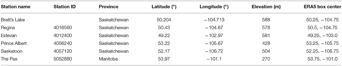
Table 1. Climate stations with location and elevation.

TABLE 2

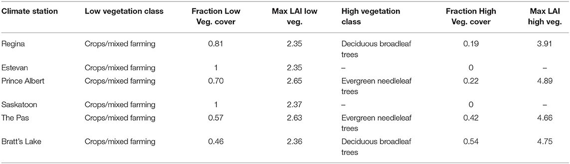
Table 2. Vegetation representation in ERA5 for the grid-box nearest to climate stations.

Data Processing

Our comparison uses daily means of temperature (T_m), together with maximum (T_x), and minimum temperature (T_n) and the diurnal range of temperature (DTR)

$\begin{array}{ll}\text{DTR}={\text{T}}_{\text{x}}-{\text{T}}_{\text{n}}& (1)\end{array}$

The reduction of the hourly Prairie data to daily means is discussed in Betts et al. (2013a). The Prairie data uses Local Standard Time (LST = UTC-6) all year, which is about an hour later than local solar time. The hourly ERA5 data was therefore shifted to LST and similarly reduced to LST daily means, and daily T_x, T_n. We also computed hourly scalar wind speed (WS) from the hourly u- and v-wind components, and calculated daily means as an average of the 24 hourly values.

We defined the bias of a variable X as the difference between the co-located ERA5 value and the climate station data.

$\begin{array}{ll}\text{bias}:\text{X}=\text{X}:\text{ERA}5-\text{X}:\text{data}& (2)\end{array}$

Note that the ERA5 value represents a mean over the model grid-box of ~485 km² (at 51°N), while the point station data comes from instruments over standard grass plots, which are located near airports. Our climatic sampling of the bias structure is excellent, as 99.97% of the days have no missing hourly data. As in Betts and Beljaars (2017) our data aggregation strategy is simply to merge the biases from the four Saskatchewan stations to maximize sample size before making sub-stratifications. The standard deviation (SD) of the long-term mean temperature biases between stations is small, of order ± 0.1°C. Later, we will discuss how the SD of the temperature biases changes with timescale.

Over mountainous terrain, station data varies strongly with location and elevation (Gultepe et al., 2014), but over the Saskatchewan Prairie sites, the small elevation difference between the ERA5 mean and the station data can be estimated from the difference in surface pressure, bias:PS, which has a mean value of −1.2 ± 1.4 hPa across the four Saskatchewan stations. Under conditions near freezing with blowing snow and icing, both temperature and precipitation data may be biased (Gultepe et al., 2014), but this long-term analysis uses the data as archived.

We will only analyze precipitation biases on monthly and longer timescales (see sections Monthly Precipitation Comparison and Monthly Temperature and Precipitation Biases). Since precipitation varies substantially on the km scale, comparing the station precipitation data on daily time-scales to the ERA5 quarter-degree mean, computed from a dynamical model, is not reasonable.

The Prairie data have also proved extremely useful because trained observers made hourly observations of the opaque cloud fraction in tenths: defined as clouds that obscured the sun, moon or stars. This was done for cloud layers and for the total sky: we use the total sky opaque cloud fraction. The observers have followed the same protocol for the past 60 years, and there are very few missing hourly observations. So that we can compare directly with the Betts et al. (2017) ERI analysis, sections Prairie Warm Season Biases to Prairie Wind Speed Biases stratify the biases by daily mean opaque cloud. In addition we initially separate the year into the cold season with snow cover, and the warm season without snow cover, since the Prairie analyses had shown the critical role of snow cover as a climate switch (Betts and Desjardins, 2018). However, the ERA5 biases proved to be much smaller than in ERI, without discontinuities across the snow-no snow boundary, so we will drop the snow cover separation for the bias corrections in section Bias Correction for ERA5 for the Prairies.

Mean opaque cloud is highly correlated with the observed diurnal cycle of temperature (Betts and Tawfik, 2016), so diurnal cycle biases of temperature from (2) indicate biases in ERA5. These may come from errors in the land surface modeling, or from model cloud cover, which affects the downward shortwave (SW) and longwave (LW) radiation estimates. We will assess the ERA5 SW and LW biases by comparison with the 12 years of high quality data from the BSRN station at Bratt's Lake, Saskatchewan (Betts et al., 2015). One key SW measure is the effective cloud transmission

$\begin{array}{ll}\text{ECT}=\text{S}{\text{W}}_{\text{dn}}/\text{SW}{\text{C}}_{\text{dn}}& (3\text{a})\end{array}$

That is, the ratio of the downward shortwave and the downward shortwave clear-sky radiation, which is the fraction of the clear-sky radiation reaching the surface. The effective cloud albedo, ECA, computed as

$\begin{array}{l}\text{ECA}=1-\text{ECT }(3\text{b})\end{array}$

is the fraction of the clear-sky radiation that is absorbed or reflected by the cloud field. We will use it as the closest model analog of the SW impact of the opaque cloud fraction.

Cloud and Seasonal Dependence of ERA5 Biases

Prairie Warm Season Biases

ERA5 data is available from 1979 and continues to the present in lagged real time. However, our comparison period is 1979–2011, because we have the climate station data for comparison through June 2011. Our partitions by snow cover are for 1979–2006, after which many snow records are missing. Following Betts and Beljaars (2017), we will show a Saskatchewan mean by averaging over the four stations Estevan, Regina, Saskatoon and Prince Albert, which form a south-north cross-section (see Table 1). The corresponding ERA5 grid-points in Table 2 have dominant low vegetation cover.

First we compare ERA5 and climate stations for the warm season with no snow cover in either ERA5 or the observations for April to October, 1979–2006. There are a total of 20,156 days. Figure 1 stratifies the biases of T_x, T_n, T_m, and DTR using ten bins for the observed daily mean fractional opaque cloud cover. We show the mean and the standard error (SE)

$\begin{array}{ll}\text{SE}=\text{SD}/\text{√N}& (4)\end{array}$

where SD is the standard deviation of the daily biases, and N is the number of days in that bin. The SE bars are small in Figure 1 because of the large sample size.

FIGURE 1

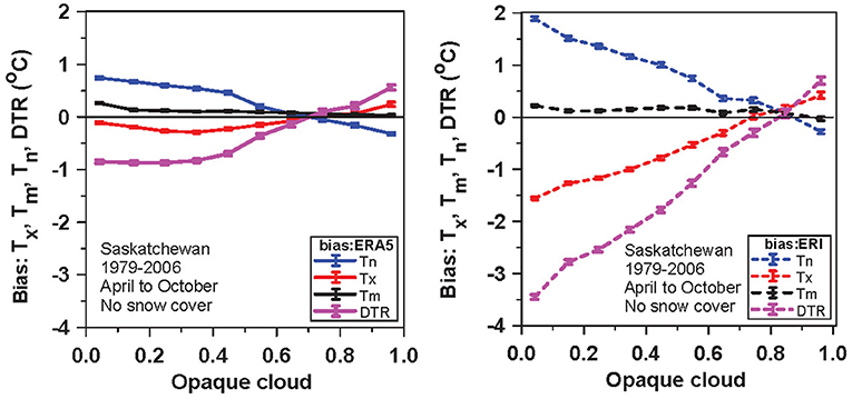
Figure 1. Opaque cloud dependence of warm season biases of T_n, T_x, T_m, and DTR for ERA5 (left) and (right) corresponding ERI biases.

Figure 1 shows the dramatic reductions in warm season bias of T_n, T_x, T_m, and DTR in ERA5 (left), compared with the ERI reanalysis (Betts and Beljaars, 2017). In ERA5, under clear skies, bias:T_n and bias:DTR only reach +0.74°C and −0.9°C respectively, while bias:T_m and bias:T_x are < −0.3°C. The primary improvements in the model land surface processes are summarized in Balsamo et al. (2011).

Figure 2 shows the seasonal cycle in the ERA5 biases in T_n, T_x (top panels) and mean T_m, DTR (bottom panels). The small warm bias in T_n increases from April to June, falls in July and August and increases again in September and October; very different from the almost monotonic increase from April to October in ERI (Betts and Beljaars, 2017). Bias:T_x decreases a little from spring to fall, while bias:T_m increases a little to +0.5^oC in fall. Bias:DTR which is dominated by bias:T_n reaches its largest negative value in October near −1.5^oC under clear skies. This is again far smaller than bias: DTR in ERI, which reaches −5°C under clear skies in October (loc cit). Clearly the 10 years of model development between ERI and ERA5 has improved the land-atmosphere coupling, and reduced the 2-m temperature biases in the analysis and 12-h forecasts by more than a factor of two under clear skies.

FIGURE 2

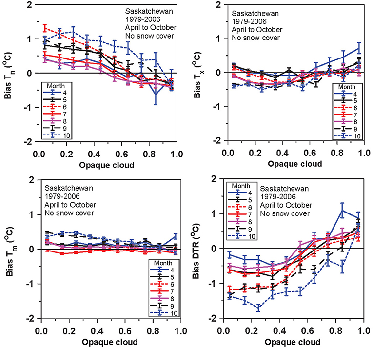
Figure 2. Opaque cloud dependence of monthly biases of T_n, T_x, T_m, and DTR.

Prairie Cold Season Biases

We merged the same four stations in Saskatchewan to examine the November to March cold season biases. We further selected only those days (12,477 days) when both ERA5 and the climate station had surface snow cover, since snow cover has such a large impact on the surface coupling (Betts et al., 2014a; Betts and Tawfik, 2016). Figure 3 shows that the cold season biases are mostly similar to those in the warm season. Bias:T_n from November to February is similar to October (Figure 2), but falls in March. Bias:T_x is very small, although we see a small positive shift in March. Bias:T_m is small and mostly positive, while Bias:DTR has similar negative values from November to February as in October (Figure 2). However, in March, Bias:DTR shifts to resemble April in Figure 2. So in ERA5, the cold season biases with snow cover are also small as in the warm season, and the structure of these small biases in general show continuity across the snow transitions.

FIGURE 3

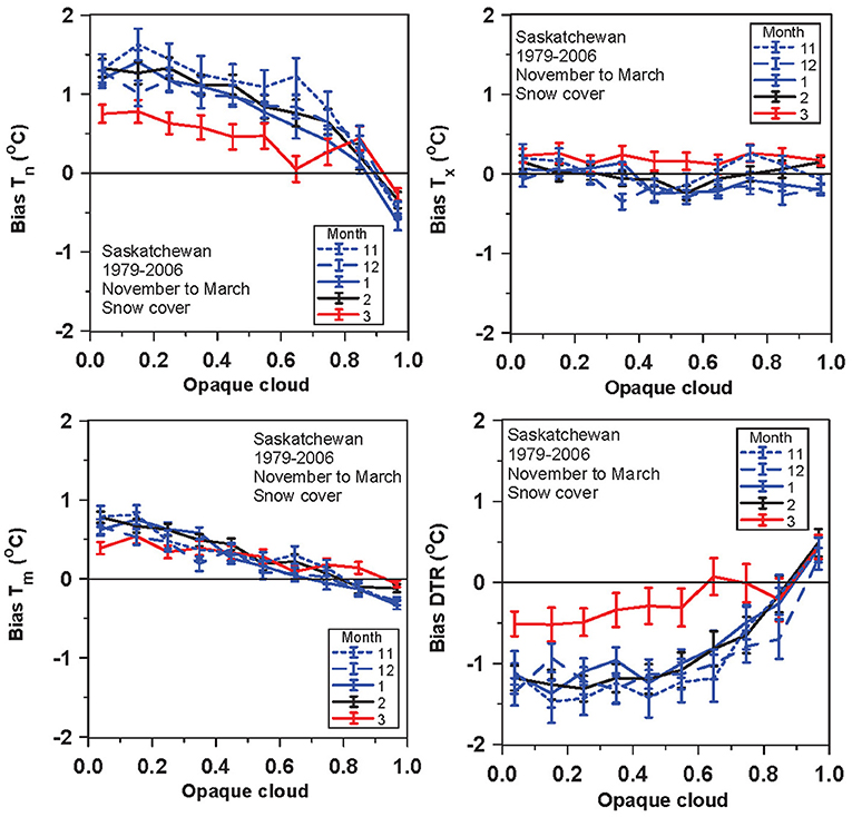
Figure 3. As Figure 2 for cold season.

In contrast in ERI (Betts and Beljaars, 2017), bias:T_x is much larger and also discontinuous between cold and warm seasons, changing under clear skies from −1.5^oC in the warm season and +1.4^oC in the cold season. Bias:T_n in ERI reaches +3^oC in January, roughly double the ERA5 bias. We conclude that there have been significant improvements in ERA5 in the snow-atmosphere coupling as well as in the warm season coupling.

Boreal Forest Contrast

The four Prairie stations in Saskatchewan are largely modeled in ERA5 as the low vegetation type, crops, and mixed farming. North of the Prairies the boreal forest is modeled largely as high vegetation, with evergreen needleleaf trees. Our climate station dataset contains a single boreal forest site at The Pas, Manitoba (Table 1). This climate station is on the south side of the airport on the south shore of Clearwater Lake, which is roughly 20 × 20 km in size. It is also in the southern half of an ERA5 grid-box with a 40% lake cover. ERA5 has a simplified model for the lake temperature profile, but the surface diurnal cycle of lake temperature is much less than over land, and this biases the ERA5 diurnal cycle substantially (not shown). We are evaluating the ERA5 lake model for Lake Champlain in northern Vermont, where we have lake data for comparison, but that work is unfinished. Here we selected for comparison with the station data the adjacent ERA5 grid-box to the south, which has no lake cover. This grid box has a high vegetation fraction of 0.42, modeled as evergreen needleleaf trees, and a low vegetation fraction of 0.57 (Table 2). Figure 4 shows (for comparison with Figures 2, 3, upper panels) the opaque cloud dependence of monthly biases of T_n and T_x in the warm season, May to October, for days with no snow cover (top panels); and November to March for days with snow cover (lower panels). At this more northern site, many more April days have snow cover, so it has been dropped from the warm season category. The biases are generally similar in magnitude to Figures 2, 3, but with only a single station, the SEs are larger. One difference is that bias:T_n is not larger in October at The Pas. Note that the SEs are typically larger in winter. The reduced bias:T_n in March seen in Figure 3 is not seen at The Pas. Our conclusion is that the biases at The Pas are similar in warm and cold seasons, and given the scatter in single station data, an annual mean is appropriate.

FIGURE 4

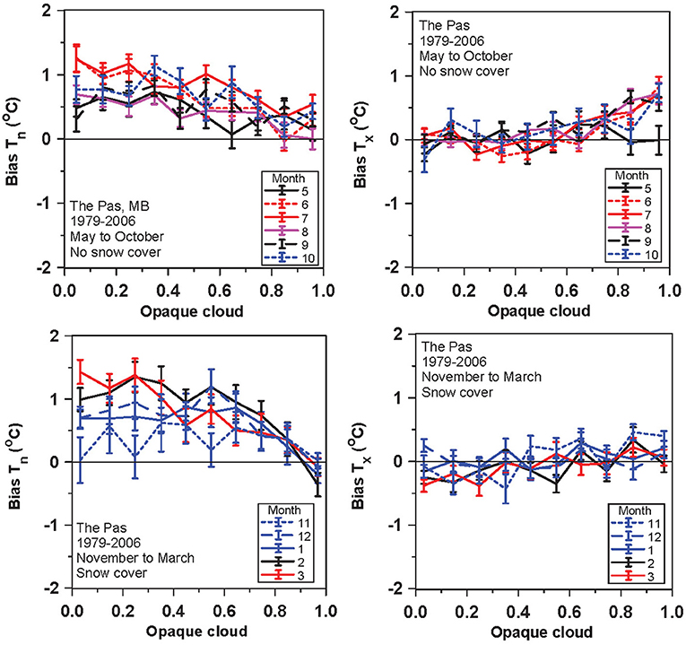
Figure 4. Opaque cloud dependence of monthly biases of T_n and T_x for The Pas in the warm season (top) and (bottom) in the cold season with snow.

Corresponding mean warm season biases in ERI for The Pas are similar to ERA5 (not shown), but in the cold season, ERI bias:T_n and bias:T_x were larger than in ERA5 by as much as +1 to +1.5^oC. Again we conclude that the ERA5 improvements in the snow-atmosphere coupling are seen over the boreal forest.

Prairie Wind Speed Biases

Figure 5 shows the mean wind speed (WS) comparison and monthly biases of wind speed plotted against daily mean opaque cloud for the warm season (left) and cold season (right), with ERA5 on top and ERI below. The top panels show that the ERA5 grid-point means are smaller than the station daily means, measured over grassland plots near airports; and there is a general increase of mean wind speed with cloud cover. The monthly mean biases derived from the daily mean scalar wind speed are all negative for ERA5. The biases are largest in April and May and smallest in July, August and September, when the variation with opaque cloud cover is small. From November to June, both wind speed and the negative bias increase with opaque cloud, and therefore with precipitation (not shown). Although there is a significant annual cycle in the wind-speed bias in ERA5, the warm and cold season biases are comparable. In section Wind Speed Bias we will show that bias:WS increases with wind speed in all seasons.

FIGURE 5

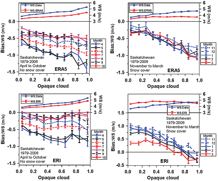
Figure 5. Mean wind speed and monthly biases of wind speed for warm season (left) and cold season (right) as a function of opaque cloud for ERA5 (top) and (bottom) ERI.

The lower comparison for ERI is adapted from Betts and Beljaars (2017). As in ERA5, the warm season (lower left) negative wind biases in ERI are largest in April and May and smallest in July, August and September. We see that the warm season bias:WS has slightly increased in ERA5. In sharp contrast to ERA5 however, bias:WS in ERI changes discontinuously across the snow cover boundary from negative to mostly positive values.

Monthly Precipitation Comparison

Figure 6 compares the mean annual cycle of precipitation for these same four stations in Saskatchewan with ERA5. In addition to the original climate station precipitation data, we have a second generation adjusted precipitation dataset by Mekis and Vincent (2011). For each rain gauge type, corrections to account for wind undercatch, evaporation, and gauge specific wetting losses were implemented. For snowfall, density corrections were applied to all snow ruler measurements.

FIGURE 6

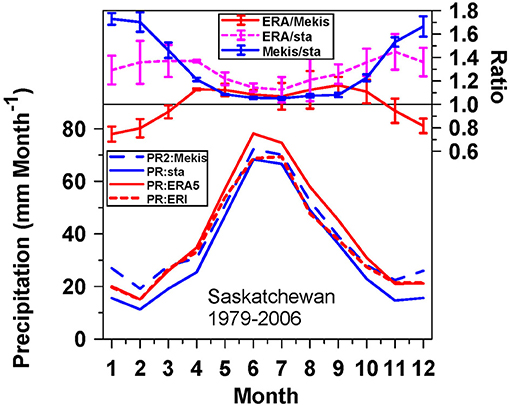
Figure 6. Mean monthly precipitation from ERA5, ERI and four climate stations in Saskatchewan (bottom) and (top) ratios of monthly mean precipitation.

The ERA5 value is a true time and space mean over each grid-box of ~485 km² at 51°N, calculated from a dynamical model run in 4-D reanalysis mode. The four climate stations are point precipitation observations, that were used to derive a second adjusted precipitation set by Mekis and Vincent (2011). The lower plots show the mean annual cycle for 1979–2006. ERA5 precipitation is greater than the unadjusted climate station precipitation (labeled PR:sta), while the Mekis adjusted precipitation lies between them from April to October, but is above ERA5 in the cold season when a large upward adjustment of snowfall is made. The corresponding monthly mean precipitation in ERI is the same as ERA5 in the cold season, when large-scale precipitation is the dominant term (not shown), but in the warm season (May to October) ERA5 has substantially more precipitation (14 ± 6%) than ERI.

We computed (Figure 6, upper plots) the three long-term ratios between ERA5 and the two datasets, and the ratio of the Mekis second generation data to the climate station precipitation data. We show the mean monthly ratios and standard deviation between the four stations.

Figure 6, upper plots, shows that ERA5 grid-point precipitation exceeds the climate station precipitation by 18 ± 5% in from May to September and by 33 ± 14% from December to February, when precipitation falls as snow. The Mekis adjusted precipitation increases precipitation by 7 ± 1% in the warm season and a much larger value averaging 70 ± 6% in winter. As a result, the ERA5 precipitation is above the Mekis estimate by about 11 ± 4% from May to September, but below it by 22 ± 7% in winter.

Our conclusions can only be tentative. The comparison in Figure 6 suggests that the Mekis correction with snow may be too large in winter, when the measurement of light snow at cold temperatures and blowing wind is challenging (Gultepe et al., 2016). However, while the model computation of precipitation is dynamically constrained, there is also a dependence on uncertainties in the model microphysical parameterization. In the warm season, ERA5 is 11 ± 4% above the Mekis dataset, which is a 7% upward correction of the station rain gauge data. Our broad conclusion, given the challenge of precipitation measurements, is that we cannot conclude that the ERA5 precipitation is biased, which is encouraging for modeling agricultural processes.

Downward Radiation Comparison

Figure 7 compares the downward radiation fluxes between ERA5 and the BSRN data. Daily mean SW_dn: ERA5 against SW_dn:BSRN (top-left), and the 1:1 line (red), show that agreement between the point BSRN observations and the ERA5 gridpoint mean is good (R² = 0.91). SW_dn:BSRN against the ERA5 clear-sky radiation estimate, SWC_dn:ERA5 is plotted top-right, and shows that 21% of the BSRN blue points lie just above the 1:1 red line for SWC_dn:ERA5. This means that the ERA5 clear-sky radiation estimates are less than the BSRN measurements under nearly-clear sky conditions over the full annual cycle. We found a similar result with ERI (Betts et al., 2015).

FIGURE 7

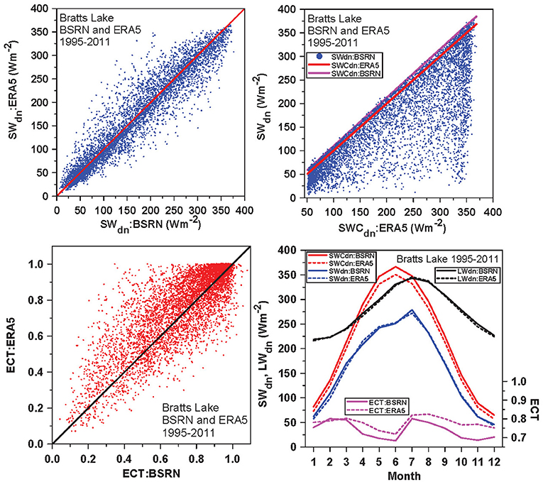
Figure 7. Daily SW_dn:ERA5 against SW_dn:BSRN (top-left); (top-right) SW_dn:BSRN against ERA5 clear-sky flux;(bottom-left) ECT:ERA5 against ECT:BSRN; and (bottom-right) Annual cycle of SWC_dn, SW_dn, LW_dn, and ECT (Equation 3a) from both ERA5 and BSRN.

We made an estimate of the BSRN clear-sky flux (purple line), by adding a small correction to SWC_dn:ERA5, which is based on Day of Year (DOY)

$\begin{array}{ll}{\text{SWC}}_{\text{dn}}:\text{BSRN}={\text{SWC}}_{\text{dn}}:\text{ERA}5+8+8*(\text{SIN}{(\text{π}*\text{DS}/365)}^{1.8}& (5)\end{array}$

where DS = DOY + 14 for DOY <351 and DOY – 351 for DOY> 350, which closely follows the procedure in Betts et al. (2016). More than 99% of the BSRN data now lies below this clear sky estimate given by (5). We computed the effective cloud transmission ECT:BSRN = SW_dn:BSRN/SWC_dn:BSRN and the bottom-left panel shows ECT: ERA5 plotted against ECT:BSRN. Over much of the range of atmospheric transmission, there are more points above the 1:1 line, suggesting that the ERA5 cloud fields reflect or absorb too little SW radiation.

The bottom-right panel shows the differences in the mean annual cycle of the downward SW and LW radiation. The difference in SWC_dn between the BSRN and ERA5 from Equation (5) ranges from 8 Wm⁻² in December to 16 Wm⁻² in June. However, the larger ECT in ERA5 reduces the differences in the mean annual cycle of the SW_dn between ERA5 and BSRN from April to December to < ±7 Wm-2. The corresponding mean monthly LW_dn for ERA5 and BSRN are very close: with the monthly mean difference ranging between −5 and +2 Wm⁻². These SW and LW differences between the ERA5 and BSRN data are small enough that we suggest that ERA5 downward radiation can be treated as unbiased for climatological purposes.

Bias Correction for ERA5 for the Prairies

Temperature Biases

The diurnal cycle biases over the Prairies, shown in Figures 1–3 as a function of the observed variable, opaque cloud, are generally largest under clear skies. However, they have been greatly reduced since our earlier study using ERI (Betts and Beljaars, 2017), as a result of 10 years of model development. The ERA5 biases show monthly variability but, unlike ERI, sharp transitions with snow cover between warm and cold seasons are no longer visible, presumably because of the improvements in the snow model in ERA5. The biases of ERA5 against the Prairie data show the sharpest relationships when binned against the observed opaque cloud cover, because of the climatic sensitivity of observed temperature to observed cloud cover (Betts et al., 2013a). However, to use ERA5 as a gridded dataset with a quarter-degree spatial resolution for agricultural studies, we need to correct the biases in ERA5 using model variables. We will use the model computed ECA from Equation (3b) as the closest model analog of opaque cloud cover.

Figure 8 (top-left) shows the annual cycle of the mean temperature biases for the four-station Saskatchewan dataset (47,477 days), with no separation for snow cover. There is a large monthly variation, but we can see some structure. Bias:T_n is largest from October to February, with minima in April and August, and a weak maximum in June. Bias:T_x has a weak positive maximum in March, but is negative for most of the year. Bias:T_m is only briefly negative in July. The corresponding monthly distribution of bias:T_n plotted against ECA is shown top-right. The blue and black plots correspond to the high monthly mean values of bias:T_n from October to February, while the lower cyan, red and magenta plots correspond to the months March to September. For clarity we show only a pair of representative SEs. The month to month variation is noisy, but generally the profiles have a similar structure with bias:T_n increasing as ECA decreases. The corresponding panels in Figures 2, 3 for bias:T_n show a smoother but similar variation with opaque cloud. Our assessment is that monthly bias correction is unrealistic, but the separation into two broad groups is a useful simplification. The March to September mean has quite small biases (bottom-left). The October to February mean biases are substantially larger (bottom-right). The linear fits, given in Equations (6, 7), are shown dotted.

FIGURE 8

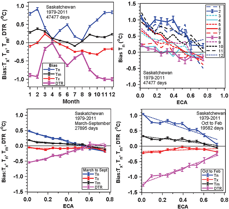
Figure 8. Monthly variation of ERA5 temperature biases (top-left), (top-right) ECA variation of monthly bias:T_n; and ECA variation of temperature biases for March to September (bottom-left) and for October to February (bottom-right).

The linear fits to the March to September Saskatchewan data in Figure 8 (bottom-left), with the ± standard error, are

$\begin{array}{ll}\text{ Bias}:{\text{T}}_{\text{x}}=-0.078(\pm 0.03)-0.03(\pm 0.06)\text{ECA}\text{(}{R}^2=0.11)& (6\text{a})\end{array}$

$\begin{array}{ll}\text{ Bias}:{\text{T}}_{\text{n}}=0.49(\pm 0.01)-0.90(\pm 0.03)\text{ECA }\text{(}{R}^2=0.99)& (6\text{b})\end{array}$

$\begin{array}{ll}\text{ Bias}:{\text{T}}_{\text{m}}=0.17(\pm 0.02)-0.32(\pm 0.04)\text{ECA }(R^2=0.84)& (6\text{c})\end{array}$

$\begin{array}{ll}\text{Bias}:\text{DTR}=-0.56(\pm 0.03)+0.86(\pm 0.07)\text{ECA }(R^2=0.94)& (6\text{d})\end{array}$

The linear fits to the October to February data in Figure 8 (bottom-right) are

$\begin{array}{ll}\text{ Bias}:{\text{T}}_{\text{x}}=-0.17(\pm 0.04)+0.13(\pm 0.09)\text{ECA }(R^2=0.10)& (7\text{a})\end{array}$

$\begin{array}{ll}\text{ Bias}:{\text{T}}_{\text{n}}=1.04(\pm 0.07)-1.12(\pm 0.17)\text{ECA }(R^2=0.83)& (7\text{b})\end{array}$

$\begin{array}{ll}\text{ Bias}:{\text{T}}_{\text{m}}=0.33(\pm 0.03)-0.41(\pm 0.08)\text{ECA }(R^2=0.72)& (7\text{c})\end{array}$

$\begin{array}{ll}\text{Bias}:\text{DTR}=-1.21(\pm 0.04)+1.25(\pm 0.10)\text{ECA }(R^2=0.94)& (7\text{d})\end{array}$

Note that for bias:T_x, the slope of these fits is not significantly different from zero.

Figure 9 shows the annual cycle and ECA distribution for The Pas (11,873 days). Figure 9 (left panel) has some similarities with Figure 8 (top left) with small biases in April and a drop in bias:T_n in August. In March and July there are signs of possible seasonal delay at this higher latitude. One difference is the sign reversal of bias:T_x, and no rise in bias:T_n from October to January. Because the seasonal changes in biases are relatively small (except in April, which we note corresponds to snowmelt), we averaged the data from all months to show the ECA distribution of the biases in the right panel. This is much flatter than in Figure 8 (lower panels) for the Prairie data. We do not know the underlying reasons in the land-atmosphere coupling for these differences in biases between the Prairie mean and this site with larger forest cover, but as noted in section Boreal Forest Contrast the cold season temperature biases are much smaller in ERA5 than ERI.

FIGURE 9

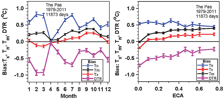
Figure 9. Monthly dependence of temperature biases for The Pas (left) and (right) ECA dependence.

Wind Speed Bias

We used the average of the same four Saskatchewan stations to explore the monthly and diurnal structure of the ERA5 wind speed bias. Figure 10 (top-left panel) shows the annual cycle of wind speeds (below) and (above) bias:WS (solid black line). Also shown (dashed) is a separation of bias:WS into mean day and night-time values, which is discussed below. It is clear that the negative bias gets larger with increasing wind speed and the daytime bias is larger than the night-time bias. The model near-surface 10-m wind is not itself a predicted variable: instead the lowest predicted model level wind is post-processed using an exposure correction to try to match observed 10-m wind (Cy41r2, 2016, Pt IV, chapter 3).

FIGURE 10

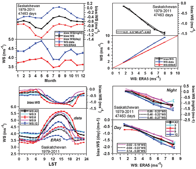
Figure 10. Annual cycle of WS:data, WS:ERA5 and day and night bias:WS (top-left) and (top-right) binned by WS:ERA5; (bottom-left) diurnal cycle of WS and bias partitioned by solar quarters, and (bottom-right) day and night bias partitioned by solar quarters.

The top-right panel shows the dependence of the bias on ERA5 wind speed and the linear fit given by

$\begin{array}{ll}\text{Bias}:\text{WS}=0.22(\pm 0.04)-0.22(\pm 0.01)*\text{WS }(R^2=0.98)& (8)\end{array}$

From Equation (8), the negative bias of the ERA5 estimate of the 10 m wind increases from 15 to 18% of WS between 3 and 6 ms⁻¹. We have insufficient data to estimate the bias:WS above 8 m/s.

The bottom-left panel shows the mean diurnal cycle of the winds and bias:ERA5 (black lines). We see a large diurnal cycle in the bias with daytime values that are larger negative than at night, consistent with the panel above. The color scheme indicates the division of the months of the year in four groups by solar zenith angle which determines day length: these we will call solar quarters. These are denoted 3, 6, 9, 12 for the central months of the month groups: (2,3,4); (5,6,7); (8,9,10); and (11,12,1). In mid-afternoon the mean bias has a mean value ≈ −1.1 ms⁻¹, which is almost identical in all four groups, but the nighttime bias is quite flat, and falls monotonically from solar quarter 12–9. We made a simple split of the diurnal cycle into day and night hours by defining the nighttime period for the solar quarters 3, 6, 9, 12, respectively, as LST hours: (21–7), (22–6), (21–7), and (18–10). We used (21–7) to split the mean bias into day and night both here and in the panel above. Our treatment is approximate as close examination shows the diurnal response of wind speed in ERA5 and the station data differ. This is clearest in quarter 6. For ERA5 the morning change from the flat nighttime bias comes at LST = 5, which is the time of minimum temperature, but the corresponding kink in the station wind data is 1 h later at LST = 6. There is a similar lag in the evening transition in the station data that then shows up as an anomalous kink in bias:WS at LST = 19. In ERA5, the night-time stable BL and daytime unstable BL use different parameterizations, and the post-processed 10-m wind appears to make both morning and evening transitions about an hour earlier (that is faster) than suggested by the station 10-m wind.

The final bottom-right panel shows the quasi-linear increase in bias:WS with WS if we split into night and day means, as well as the further division into the four solar quarters. Remarkably we see similar patterns with similar slopes for day and night with a mean upward shift (reduction of negative bias) of 0.5 ms⁻¹ at night. Seasonally we see the negative bias:WS is larger both day and night in quarter 12, but reduced in quarter 9. These wind speed biases have a systematic diurnal and seasonal structure, which could provide conceptual guidance for improvements in the model post-processed 10-m wind.

Standard Deviation of Biases on Shorter Time-Scales

Daily and 5-Day Mean Temperature Biases

Section Bias Correction for ERA5 for the Prairies addresses the correction of the small ERA5 systematic biases derived from long-term climatological datasets. The standard errors shown on Figures 8, 9 are small because we have averaged these very large datasets. However, the root-mean-square temperature differences between the reanalysis and point station data on daily timescales are much larger. Figure 11 (left panel) shows the standard deviation of the daily biases, plotted against ECA (lower plots), showing SD(bias:T_m) reaching 0.9°C under clear skies, with larger SDs for bias:T_x, bias:T_n, and bias:DTR. The upper scatterplot is daily opaque cloud against daily ECA, and the heavy black line is the mean and SD of opaque cloud, plotted against binned ECA. For reference, the light solid line is the 1-to-1 line of ECA. On daily timescales, the station opaque cloud, and grid-box mean ECA are poorly correlated, as seen in Figure 7 for ECT at the BSRN site. Figure 11 (right panel) is the corresponding plot for 5-day means, and we see a large drop in the SDs of the temperature biases and the scatter of opaque cloud on ECA. So on the longer timescales that are important for agricultural modeling, the SD of the temperature biases fall substantially.

FIGURE 11

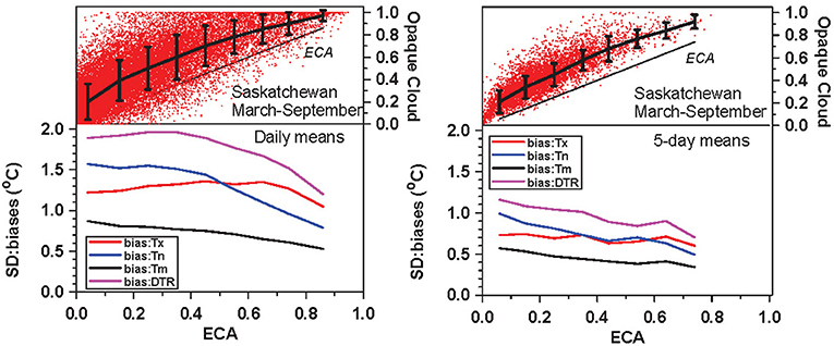
Figure 11. (Left) Daily standard deviation of temperature biases (lower plots) and daily opaque cloud (upper plot) and (right) corresponding plot for 5-day means.

Daily timescale comparisons are noisy because different space and timescales are involved, as well as advective processes. The daily climate station point data is sampled every hour with an upstream 24-h advection distance of 346 km at 4 ms⁻¹. The ERA5 boxes are quarter-degree mean values sampled hourly. ERA5 does not give a good prediction of daily cloud cover at climate stations, and this contributes to the larger SDs of the temperature biases. However, the relationship between cloud cover and the diurnal cycle, which is well-defined in climatological means (e.g., Betts and Tawfik, 2016) is itself noisy on daily timescales (not shown).

Monthly Temperature and Precipitation Biases

Figure 12 shows the relation between climate station temperature and precipitation on monthly timescales for the months May to September when snowfall is rare. There are 758 months on these plots. For T_m, we just show the 1:1 line because the linear fit is almost indistinguishable. In comparison with Figure 11, the monthly SD of bias:T_m falls to ±0.3°C, and to ± 0.5°C for T_x and T_n (not shown). The comparison of monthly climate station precipitation with ERA5 shows large scatter. The point station data is not representative of the ERA5 gridbox, because precipitation varies substantially on the km scale. Extremes of station precipitation can occur locally even in monthly sums: note for example the four high station precipitation values to the lower right. The monthly SD of bias:Precip is 22 mm Month⁻¹. Linear fits are of no value with this scatter, so we show the reference line for the +18% long-term bias in ERA5 for May to September, derived from Figure 6.

FIGURE 12

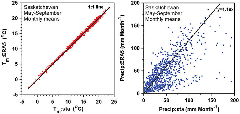
Figure 12. Monthly mean ERA5 temperature data against station data (left) and (right) the same for monthly precipitation.

The small temperature biases in both 5-day and monthly means, shown in Figures 11, 12, suggest that ERA5 air temperature data should be very useful for modeling certain agricultural processes. However, we cannot realistically assess the ERA5 precipitation on monthly timescales from the station data, given the large SD of monthly bias:Precip. Comparison of ERA5 precipitation with other spatially distributed precipitation estimates from radar composites and satellite products would be useful.

Energy and Water Balance in ERA5

The value of reanalyses is that they provide the terms in the energy and water budgets, as well as the meteorological fields. This section shows the mean monthly surface energy and water budgets averaged over the four ERA5 grid-points for Estevan, Regina, Saskatoon and Prince Albert, Saskatchewan. Table 2 shows that crops/mixed farming is the dominant vegetation cover.

We derived the residual G in the surface energy balance

$\begin{array}{ll}\text{G}={\text{R}}_{\text{net}}+\text{SH}+\text{LH}& (9)\end{array}$

where R_net, SH, and LH are the surface net radiation, sensible heat flux and latent heat flux, which are all defined positive downward (that is, upward SH and LH are negative in the model notation). In the warm season G is the soil heat flux; with snow cover, G contributes also to the energy balance of the snow layer, including snow melt. We derived the monthly means for the 35 years in our ERA5 reanalysis period, 1979–2013. From these we calculated the monthly mean surface albedo as

$\begin{array}{ll}\text{Albedo}=(\text{S}{\text{W}}_{\text{dn}}-\text{S}{\text{W}}_{\text{net}})/\text{S}{\text{W}}_{\text{dn}}& (10)\end{array}$

For the months, April to September, we computed the monthly mean evaporative fraction,

$\begin{array}{ll}\text{EF}=\text{LH}/(\text{LH }+\text{ SH})& (11)\end{array}$

Figure 13 (top panels) shows the mean annual cycle of the terms in Equations (9–11) for this Saskatchewan mean. With 4 stations and 35 years of data, the error bars are the SE calculated from the SD of the 140 monthly means using (4), with √N = 11.8. SW_net, R_net, and LH peak in July, while SH, which rises with LH in spring, peaks earlier in May, when evapotranspiration takes over. The EF peaks in July, and the summer (JJA) mean in ERA5 is 0.73. The mean albedo for the May to August (MJJA) growing season is 0.17 and in winter (DJF) with snow cover, mean albedo is 0.57. The upper plot in the top-right panel shows the relation between the DJF snow depth, represented as snow water equivalent (SWE), and the corresponding four-station-mean albedo for the 35 winters. The heavy line is the quadratic fit which shows that albedo plateaus at 0.7 with SWE = 35 mm. The two ERA5 grid-boxes with tall vegetation that shades the snow, Regina and Prince Albert, have reduced albedo (not shown). It would be useful to intercompare the ERA5 coupling of winter albedo to vegetation and snow cover with albedo values derived from MODIS data (Khlopenkov and Trishchenko, 2008; Luo et al., 2008).

FIGURE 13

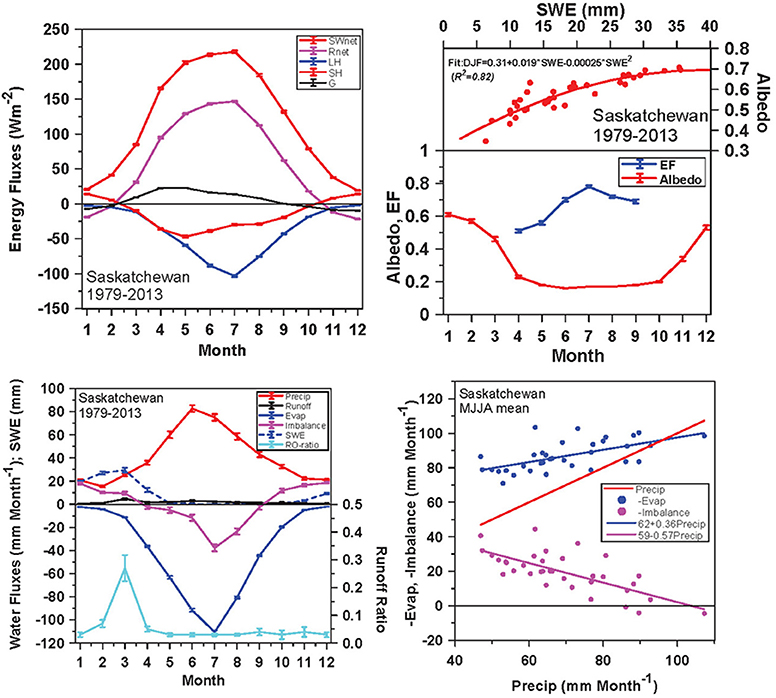
Figure 13. Annual cycle of terms in the surface energy balance (top-left) and (top-right) albedo and EF and annual winter coupling of albedo to SWE; (bottom-left) the surface water balance, SWE and runoff ratio, and (bottom-right) the interannual coupling of MJJA precipitation, evaporation, and surface water imbalance.

For the water budget in mm Month⁻¹, precipitation peaks in June and evaporation (actually evapotranspiration) peaks in July. We computed the monthly Imbalance as

$\begin{array}{ll}\text{Imbalance}=\text{Precip}-\text{Runoff}+\text{Evap}& (12)\end{array}$

where we have abbreviated precipitation and evaporation. Figure 13 (bottom-left) shows the mean annual cycle of the terms in Equation (12), and SWE. The Imbalance is small over the annual cycle, but negative in the MJJA growing season, when (-Evap) > Precip by 38 mm Month⁻¹ in July. This comes primarily from the drawdown of deep soil water (the total model soil depth is 289 cm). We show also the Runoff Ratio = Runoff/Precip, which is ≈ 0.03 for MJJA, but reaches 0.27 during spring melt in March. In some years, snowmelt exceeds precipitation in spring.

The reanalysis does not strictly conserve water or heat in the soil, because the soil moisture analysis adds increments of soil moisture and soil temperature to minimize the errors in the 2-m air temperature over the diurnal cycle. For G the 35-y mean annual residual is +5 W/m². The mean annual residual of the Imbalance is only 0.1 ± 5.0 mm Month⁻¹; meaning that precipitation, evaporation and runoff closely balance in the long run, even though there is substantial variability in the annual mean.

The interannual variability of the warm season imbalance plays a major role in the growing season. The bottom-right panel plots MJJA evaporation and water imbalance, both with reversed sign, against precipitation for the four Saskatchewan station mean for each of the 35 years. Mean growing season precipitation ranges from 47 to 107 mm Month⁻¹, with a mean of 69.2 ± 14.6 mm Month⁻¹. The range of evaporation is smaller, only −71 to −103 mm Month⁻¹, with a mean of −86.5 ± 8.5 mm Month⁻¹. The long-term MJJA runoff mean is 2.2 ± 2.6 mm Month⁻¹. However, MJJA runoff is only 0.9 ± 0.5 mm Month⁻¹ in the first two decades of the reanalysis, but since 2000 the mean has increased to 4.1 ± 3.3 mm Month⁻¹. This suggests further model analysis is needed, since we can see no simple explanation.

The imbalance, with a mean of −19.5 ± 11.6 mm Month⁻¹, primarily the extraction of deep soil water, effectively damps the variation in evaporation between drought and heavy rain years. We show the linear fits to the annual MJJA evaporation and imbalance for comparison with Betts et al. (2014b). They used the gravity satellite (GRACE) data to estimate the slope of the MJJA drawdown of total water storage on the Prairies as −0.59 ± 0.09 (R² = 0.56), comparable to the value here in the ERA5 water imbalance of −0.57 ± 0.10 (R² = 0.51). The linear fit here for evaporation on precipitation (in mm Month⁻¹) has a slope of 0.36 ± 0.08 (R² = 0.37), comparable to the residual estimate in Betts et al. (2014b) of 0.39 ± 0.09, who fixed the MJJA runoff ratio at 0.05.

Our conclusion is that the ERA5 surface energy and water fluxes appear to have a realistic annual variation. Two types of deeper assessments are possible, although we leave them to future work. The ERA5 surface fluxes, specifically the total evapotranspiration could be compared with estimates from agricultural models driven by bias-corrected ERA5 data. Comparisons with flux stations (FLUXNET Canada, 2016) would also be useful.

Conclusions

By comparing data from four climate stations on the Saskatchewan Prairies with corresponding grid-points in the ERA5 reanalysis, we have explored the model biases in the mean diurnal cycle of temperature, represented by T_x, T_n, T_m, and DTR. First we binned the biases by opaque cloud cover, separating the warm season without snow cover, and the cold season with snow cover to make a direct comparison with an earlier study using ERI (Betts and Beljaars, 2017). Compared with ERI, the biases in ERA5 have been greatly reduced in warm and cold seasons, and no longer show large differences with snow cover. We compared the ERA5 biases for a grid-box within the boreal forest at The Pas; and found biases that are broadly similar to our Saskatchewan Prairie mean, which also change little between winter and summer. For both the Prairies and our one boreal forest site, it is clear that improvements to the snow model between ERI and ERA5 have removed large erroneous diurnal cycle biases with snow. We computed fits to the ERA5 mean temperature biases as a function of ERA5 effective cloud albedo. These mean corrections are small: < 0.2^oC for T_x, < 0.3^oC for T_m, and < 0.8^oC for T_n. They can be used to improve slightly the ERA5 diurnal cycle of temperature for agricultural modeling.

In contrast, the ERA5 has a negative wind speed bias in the warm season that is slightly worse than in ERI. However, in the cold season with snow the ERA5 negative wind bias is similar to the warm season, whereas ERI has a discontinuous change in wind bias across the snow cover boundary. We investigated the diurnal and seasonal structure and found that bias:WS is larger in the daytime than at night. The negative wind bias also increases quasi-linearly with wind speed, both day and night and in all seasons; increasing from 15 to 18% of WS between 3 and 6 ms⁻¹. Because these wind speed biases have a systematic diurnal and seasonal structure, we suggest they could provide conceptual guidance for improvements in the post-processed 10-m wind in the model.

We used data from a BSRN site near Regina to show that the biases in the downwelling shortwave and longwave radiation fluxes in ERA5 are small under clear skies, and have changed little from ERI. The BSRN data suggest that daily mean ERA5 downward clear-sky radiation is lower by −8 Wm⁻² in December and −16 Wm⁻² in June, but lower cloud cover in ERA5 than in the BSRN data means that the bias in the downward SW radiation is small. The downward LW radiation in ERA5 is also almost unbiased.

We evaluate ERA5 precipitation against the original climate station precipitation data, and a second generation adjusted precipitation dataset by Mekis and Vincent (2011). Compared to ERI, ERA5 has the same monthly mean precipitation in the cold season, when large-scale precipitation is the dominant term, but substantially more (14 ± 6%) in the warm season. For May to September ERA5 has a bias of 18 ± 5% above the station data and 11 ± 4% above the Mekis dataset, which adjusts precipitation upward by 7 ± 1% in this warm season. In winter with snowfall, the Mekis upward precipitation adjustment is much larger, averaging 70 ± 6%. The Mekis correction with snow may be too large, as ERA5 is−22 ± 7% below their estimate in winter. Assessing whether the ERA5 precipitation is biased is unrealistic, since precipitation varies substantially on the km scale. For May to September the SD of ERA5 monthly bias:Precip is large: ±22 mm Month⁻¹. Given the uncertainty in point precipitation measurements, our broad conclusion is that we are unable to conclude whether the ERA5 precipitation is biased, which gives some encouragement for agricultural modeling.

We showed that the annual cycle of the surface energy and water budgets in ERA5 are realistic for the mean of our four Saskatchewan station grid-points. In particular the damping of extremes in precipitation by the extraction of soil water is comparable in ERA5 to our observational estimate in an earlier study based on GRACE satellite data (Betts et al., 2014b).

One important issue is whether data from reanalysis are sufficiently accurate to replace observations for regions in Canada, and elsewhere on the globe, where there is limited station data. On monthly timescales, mean temperature biases in ERA5 are small, of order ±0.3^oC. However, the model forecast of daily cloud cover has a large scatter compared to opaque cloud observations, which results in bias:T_x and bias:T_n having a SD ≈ 1.4°C on daily timescales. These SDs fall below 1°C in 5-day means, and fall further to ±0.5^oC in monthly means. This suggests that the reanalysis temperature data is now much better for agricultural modeling. Assessing precipitation is more challenging, given the large SD of monthly bias:Precip, and the small scale representivity of the station data, discussed earlier. Nonetheless because of its complete spatial coverage and improved accuracy, global model forecast data is now routinely used for hydrological forecasting (ECMWF, 2017).

This analysis has greatly helped identify the variables that are most affected by biases. Now we can look at the main drivers of various models to determine which agricultural model estimates are likely to be more affected. Two further assessments of the reanalysis are possible, although we leave them to future work. The ERA5 surface fluxes, specifically the total evapotranspiration, could be compared with estimates from agricultural models driven by bias-corrected ERA5 data. Comparisons with flux stations (FLUXNET Canada, 2016) would also be useful.

Data Availability

Publicly available datasets were analyzed in this study. This data can be found here: The Canadian Prairie data are available from the first author, or from Environment and Climate Change Canada at http://climate.weather.gc.ca/. The ERA5 reanalysis data are available from the Copernicus data store at https://cds.climate.copernicus.eu/cdsapp#!/dataset/reanalysis-era5-single-levels?tab=form.

Author Contributions

AB: conceptualization, analysis, writing, review, and editing. DC: software, data curation, and review. RD: conceptualization, review and editing, funding acquisition, and project administration.

Funding

This work was partially supported by the Sustainability Metric Project of Agriculture and Agri-Food Canada.

Conflict of Interest Statement

The authors declare that the research was conducted in the absence of any commercial or financial relationships that could be construed as a potential conflict of interest.

Acknowledgments

We are very grateful for technical support from Devon Worth. We are grateful to the Canadian station observers who have made hourly climate observations for many decades.

References

Albergel, C., Balsamo, G., de Rosnay, P., Muñoz Sabater, J., and Boussetta, S. (2012). A bare ground evaporation revision in the ECMWF land-surface scheme: evaluation of its impact using ground soil moisture and satellite microwave data. Hydrol. Earth Syst. Sci. 16, 3607–3620. doi: 10.5194/hess-16-3607-2012

CrossRef Full Text | Google Scholar

Balsamo, G., Boussetta, S., Dutra, E., Beljaars, A., Viterbo, P., and den Hurk, B. V. (2011). Evolution of land-surface processes in the IFS. ECMWF Newsletter 127, 12–22. Available online at: https://www.ecmwf.int/en/elibrary/14596-newsletter-no-127-spring-2011

Balsamo, G., Viterbo, P., Beljaars, A., van den Hurk, B., Hirschi, M., Betts, A. K., et al. (2009). A revised hydrology for the ECMWF model: verification from field site to terrestrial water storage and impact in the integrated forecast system. J. Hydrometeorol. 10, 623–643. doi: 10.1175/2008JHM1068.1

CrossRef Full Text | Google Scholar

Betts, A., Viterbo, P., Beljaars, A., and Van den Hurk, B. J. J. M. (2001). Impact of BOREAS on the ECMWF forecast model, J. Geophys. Res. 106D, 33593–33604. doi: 10.1029/2001JD900056

CrossRef Full Text | Google Scholar

Betts, A. K., and Ball, J. H. (1997). Albedo over the boreal forest. J. Geophys. Res. 102, 28901–28910. doi: 10.1029/96JD03876

CrossRef Full Text | Google Scholar

Betts, A. K., and Beljaars, A. C. M. (2017). Analysis of near-surface biases in ERA-Interim over the Canadian Prairies. J. Adv. Model. Earth Syst. 9, 2158–2173. doi: 10.1002/2017MS001025

CrossRef Full Text | Google Scholar

Betts, A. K., Desjardins, R., Beljaars, A. C. M., and Tawfik, A. (2015). Observational study of land-surface-cloud-atmosphere coupling on daily timescales. Front. Earth Sci. 3:13. doi: 10.3389/feart.2015.00013

CrossRef Full Text | Google Scholar

Betts, A. K., Desjardins, R., and Worth, D. (2013a), Cloud radiative forcing of the diurnal cycle climate of the Canadian Prairies. J. Geophys. Res. Atmos. 118, 1–19. doi: 10.1002/jgrd.50593

CrossRef Full Text | Google Scholar

Betts, A. K., Desjardins, R., and Worth, D. (2016). The impact of clouds, land use and snow cover on climate in the Canadian Prairies. Adv. Sci. Res. 1, 1–6. doi: 10.5194/asr-13-37-2016

CrossRef Full Text | Google Scholar

Betts, A. K., Desjardins, R., Worth, D., and Beckage, B. (2014b). Climate coupling between temperature, humidity, precipitation and cloud cover over the Canadian Prairies. J. Geophys. Res. Atmos. 119, 13305–13326. doi: 10.1002/2014JD022511

CrossRef Full Text | Google Scholar

Betts, A. K., Desjardins, R., Worth, D., and Cerkowniak, D. (2013b). Impact of land use change on the diurnal cycle climate of the Canadian Prairies, J. Geophys. Res. Atmos. 118, 11,996–12,011. doi: 10.1002/2013JD020717

CrossRef Full Text | Google Scholar

Betts, A. K., Desjardins, R., Worth, D., Wang, S., and Li, J. (2014a). Coupling of winter climate transitions to snow and clouds over the Prairies. J. Geophys. Res. Atmos. 119, 1118–1139. doi: 10.1002/2013JD021168

CrossRef Full Text | Google Scholar

Betts, A. K., and Desjardins, R. L. (2018). Understanding land-atmosphere-climate coupling from the canadian Prairie dataset. Environments 5:129. doi: 10.3390/environments5120129

CrossRef Full Text | Google Scholar

Betts, A. K., and Tawfik, A. B. (2016). Annual climatology of the diurnal cycle on the canadian prairies. Front. Earth Sci. 4:1. doi: 10.3389/feart.2016.00001

CrossRef Full Text | Google Scholar

Betts, A. K., Tawfik, A. B., and Desjardins, R. L. (2017). Revisiting hydrometeorology using cloud and climate observations. J. Hydrometeor. 18, 939–955. doi: 10.1175/JHM-D-16-0203.1

CrossRef Full Text | Google Scholar

Boussetta, S., Balsamo, G., Beljaars, A., Kral, T., and Jarlan, L. (2013). Impact of a satellite-derived Leaf Area Index monthly climatology in a global numerical weather prediction model. Int. J. Rem. Sens. 34, 3520–3542. doi: 10.1080/01431161.2012.716543

CrossRef Full Text | Google Scholar

C3S Copernicus Climate Change Service (2017). ERA5: Fifth Generation of ECMWF Atmospheric Reanalyses of the Global Climate. Copernicus Climate Change Service Climate Data Store (CDS). Available online at: https://cds.climate.copernicus.eu/cdsapp#!/home (accessed March 2019).

Cy41r2 (2016). “Part IV, Physical Processes,” in Part II, Data Assimilation, Chapter 9. Available online at: https://www.ecmwf.int/en/publications/search/?solrsort=sort_label%20asc&secondary_title=%22IFS%20Documentation%20CY41R2%22

de Rosnay, P., Drusch, M., Balsamo, G., Albergel, C., and Isaksen, L. (2011). Extended Kalman filter soil-moisture analysis in the IFS. ECMWF Newslett. 127, 12–16. Available online at: https://www.ecmwf.int/en/elibrary/14596-newsletter-no-127-spring-2011

de Rosnay, P., Drusch, M., Vasiljevic, D., Balsamo, G., Albergel, C., and Isaksen, L. (2013). A simplified extended Kalman filter for the global operational soil moisture analysis at ECMWF. Q. J. R. Meteorol. Soc. 139, 1199–1213. doi: 10.1002/qj.2023

CrossRef Full Text | Google Scholar

Dee, D. P., Uppala, S. M., Simmons, A. J., Berrisford, P., Poli, P., Kobayashi, S., et al. (2011). The ERA-Interim reanalysis: configuration and performance of the data assimilation system. Quart. J. Roy. Meteorol. Soc. 137, 553–597. doi: 10.1002/qj.828

CrossRef Full Text | Google Scholar

Desjardins, R. L., Kulshreshtha, S. N., Junkins, B., Smith, W., Grant, B., and Boehm, M. (2001). Canadian greenhouse gas mitigation options in agriculture. Nutrient Cycl. Agroecosyst. 60, 317–326. doi: 10.1023/A:1012697912871

CrossRef Full Text | Google Scholar

Desjardins, S. R. L. W., Grant, B., Campbell, C., and Riznek, R. (2005). Management strategies to sequester carbon in agricultural soils and mitigation greenhouse gas emissions. Climatic Change. 70, 283–297. doi: 10.1007/s10584-005-5951-y

CrossRef Full Text | Google Scholar

Drusch, M., Scipal, K., de Rosnay, P., Balsamo, G., Andersson, E., Bougeault, P., et al. (2009). Towards a kalman filter based soil moisture analysis system for the operational ECMWF Integrated Forecast System. G. Res. Lett. 36L:L10401. doi: 10.1029/2009GL037716

CrossRef Full Text | Google Scholar

Dutra, E., Balsamo, G., Viterbo, P., Miranda, P. M., Beljaars, A., Schär, C., et al. (2010). An improved snow scheme for the ECMWF land surface model: description and offline validation. J. Hydrometeor. 11, 899–916. doi: 10.1175/2010JHM1249.1

CrossRef Full Text | Google Scholar

ECMWF (2017). South Asia Floods Put New GloFAS River discharge forecasts to the Test. Available online at: https://www.ecmwf.int/en/about/media-centre/focus/south-asia-floods-put-new-glofas-river-discharge-forecasts-test.

FLUXNET Canada (2016). FLUXNET-Canada Research Network - Canadian Carbon Program Data Collection, 1993–2014, ORNL DAAC, Oak Ridge: Tenn.

Google Scholar

Gultepe, I., Isaac, G. A., Joe, P., Kucera, P., Thériault, J., and Fisico, T. (2014). Roundhouse (RND) Mountain Top Research Site: Measurements and Uncertainties for Winter Alpine Weather Conditions. J. Appl. Geophys. 171, 59–85. doi: 10.1007/s00024-012-0582-5

CrossRef Full Text | Google Scholar

Gultepe, I., Rabin, R., Ware, R., and Pavolonis, M. (2016). Light snow precipitation and effects on weather and climate. Adv. Geophys. 57, 147–210. doi: 10.1016/bs.agph.2016.09.001

CrossRef Full Text | Google Scholar

Haiden, T., Janousek, M., Bidlot, J., Ferranti, L., Prates, F., Vitart, F. S., et al. (2016). Evaluation of ECMWF Forecasts, Including the 2016 Resolution Upgrade. ECMWF, Technical Memorandum 792.

Google Scholar

Holtslag, A. A. M., Svensson, G., Baas, P., Basu, S., Beare, B., Beljaars, A., et al. (2013). Stable atmospheric boundary layers and diurnal cycles: challenges for weather and climate models. Bull. Amer. Meteor. 94, 1691–1706. doi: 10.1175/BAMS-D-11-00187.1

CrossRef Full Text | Google Scholar

Khlopenkov, K. V., and Trishchenko, A. P. (2008). Implementation and evaluation of concurrent gradient search method for reprojection of MODIS Level 1B imagery. IEEE Trans. Geosci. Remote Sens. 46, 2016–2027. doi: 10.1109/TGRS.2008.916633

CrossRef Full Text | Google Scholar

Loveland, T. R., Reed, B. C., Brown, J. F., Ohlen, D. O., Zhu, Z., Youing, L., et al. (2000). Development of a global land cover characteristics database and IGB6 DISCover from the 1 km AVHRR data. Int. J. Remote Sens. 21, 1303–1330. doi: 10.1080/014311600210191

CrossRef Full Text | Google Scholar

Luo, Y., Trishchenko, A. P., and Khlopenkov, K. V. (2008). Developing clear-sky, cloud and cloud shadow mask for producing clear-sky composites at 250-meter spatial resolution for the seven MODIS land bands over Canada and North America. Remote Sens. Environ. 112, 4167–4185. doi: 10.1016/j.rse.2008.06.010

CrossRef Full Text | Google Scholar

Mekis, É., Donaldson, N., Reid, J., Zucconi, A., Hoover, J., Li, Q., et al. (2018). An overview of surface-based precipitation observations at environment and climate change Canada. Atmos.-Ocean 56, 71–95. doi: 10.1080/07055900.2018.1433627

CrossRef Full Text | Google Scholar

Mekis, É., and Vincent, L. A. (2011). An overview of the second generation adjusted daily precipitation dataset for trend analysis in Canada, Atmos.-Ocean. 49, 163–177. doi: 10.1080/07055900.2011.583910

CrossRef Full Text | Google Scholar

Smith, W. N., Grant, B. B., Desjardins, R. L., Kröbel, R., Qian, B., Worth, D. E., et al. (2013). Assessing the effects of climate change on crop production and GHG emissions in Canada. Agricult. Ecosyst. Environ. 179, 139–150. doi: 10.1016/j.agee.2013.08.015

CrossRef Full Text | Google Scholar

Smith, W. N., Grant, B. B., Desjardins, R. L., Qian, B., Hutchinson, J. J., and Gameda, S. B. (2009). Potential impact of climate change on carbon in agricultural soils in Canada, 2000-2099. Climatic Change 93, 319–329. doi: 10.1007/s10584-008-9493-y

CrossRef Full Text | Google Scholar

Van den Hurk, B. J. J., Viterbo, P., Beljaars, A. C. M., and Betts, A. K. (2000). Offline Validation of the ERA40 Surface Scheme. ECMWF Tech Memo, 295, 43 pp., Eur. Cent. For Medium-Range Weather Forecasts, Shinfield Park, Reading RG2 9AX, England, UK. Available online at: https://www.ecmwf.int/en/elibrary/12900-offline-validation-era40-surface-scheme

Viterbo, P., and Beljaars, A. C. M. (1995). An Improved Land Surface Parametrization Scheme in the ECMWF Model and Its Validation. ECMWF Tech. Report No. 75, Research Department, ECMWF.

Google Scholar

Viterbo, P. A., Beljaars, C. M. J., Mahfouf, F., and Teixeira, J. (1999). The representation of soil moisture freezing and its impact on the stable boundary layer. Quart. J. Roy. Meteor. Soc. 125, 2401–2426. doi: 10.1256/smsqj.55903

CrossRef Full Text | Google Scholar