A Rigorous Statistical Assessment of Recent Trends in Intensity of Heavy Precipitation Over Germany

1. Introduction

During the past decades, climate change has been one of the most intensively discussed topics in atmospheric science. The drivers behind the debates not only include the question of whether or why climate change is occurring, but also the assessment of the potential impacts of climate change on nature and society. This applies in particular to changes in the frequency and intensity of meteorological extreme events such as droughts, heat waves, and heavy precipitation events, as these directly endanger people's health and can cause tremendous damage to nature and infrastructure. Quantifying the future risk and potential intensity of such extreme events is thus of high social and economic relevance. However, assessing the risks of future climate extremes requires a reliable and robust statistical framework. Otherwise, the results could lead to false decision making in risk management.

The robustness and reliability of a statistical framework for extreme events can be evaluated by considering three main relevant aspects:

1. The definition of an extreme event. The special report on extreme events (SREX) by the Intergovernmental Panel on Climate Change (IPCC, 2012) defines an extreme event as the occurrence of a value of a weather or climate variable above/below a threshold value near the upper/lower ends of the observed distribution of the respective variable. However, there are usually no common values for the thresholds themselves. In turn, these must be specifically defined in each statistical framework. A poorly defined threshold could either exclude events that might be considered extreme or include too many events that are not extreme and thus may lead to a bias in the results.

2. Insensitivity against small deviations from the assumptions (Huber and Ronchetti, 2009). This includes prior assumptions on the underlying distribution of the data (e.g., in Bayesian inference), fitting a distribution to the data (e.g., Zolina et al., 2008) or the assumption of independent and identically distributed (iid) data (e.g., in linear regression).

3. Robustness against outliers.

All three characteristics significantly influence the result of a statistical assessment and are usually present in most common statistics for analyzing extreme events. Therefore, they can be seen as a natural source of uncertainty in every statistical framework for extreme events, independent of the applied method.

In the context of climate research, two widely applied statistical frameworks based on the concepts of extreme value statistics (EVS) are block maxima (BM; Fisher and Tippett, 1928) and the peak-over-threshold (POT; Coles, 2001) approach. Both methods aim to approximate the probability density function (PDF) by fitting a generalized parent distribution to a series of extreme events, where an extreme event is defined as either the maximum of a certain time period (for BM) or as each value above a given threshold (for POT). Hence, BM and POT systematically reduce the data via their intrinsic definition of an extreme event. However, fitting distributions require a sufficient amount of data, otherwise the parameter estimation is subject to large variances. Therefore, depending on the definition of an extreme event and the length of the underlying time series, reducing the data could add another aspect to the already described sources of uncertainty.

Given the current state of the art and accounting for the potential sources of uncertainty, robust, and reliable alternatives are necessary to corroborate or expand knowledge on climate change impact. Here, we propose quantile regression (QR) as a possible alternative. QR is a statistical regression tool that enables the estimation of non-stationary quantile curves and, thus, the investigation of the full distribution of any desired variable. It was first introduced by Koenker and Bassett (1978) and has multiple advantages compared to classical regression methods. For example, QR makes no assumptions about the underlying distribution and is equivariant to monotone transformations of the underlying data. Furthermore, QR does not require a pre-processing of the data for the sake of defining extreme events. By using quantiles, an extreme event is solely defined by a given probability of occurrence. This probability does not affect the sample size, because QR always uses all the data to estimate non-stationary quantiles. The definition of an extreme event does therefore not affect the sample size or its properties. This further motivates the use of QR in EVS. The method also proved to be extremely robust against outliers (John, 2015).

QR has already been widely applied in various studies in economics (Machado and Mata, 2005; Coad and Rao, 2008), medicine (Austin et al., 2005; Ding et al., 2010), survival analysis (Koenker and Geling, 2001; Peng and Huang, 2008), and many other fields. Applications to extreme events include the analysis of sea level (Barbosa, 2008; Donner et al., 2012; Ribeiro et al., 2014) and air temperature trends (Barbosa et al., 2011; Gao and Franzke, 2017; Rhines et al., 2017; Haugen et al., 2018), the increase in the intensity of tropical cyclones (Elsner et al., 2008), or the scaling of extreme precipitation with temperature (Wasko and Sharma, 2014).

In this article, we further demonstrate the proficiency of QR and its potential of being a complementary and powerful statistical tool for non-stationary extreme value analysis through the study of recent trends in the intensity of heavy precipitation over Germany. In order to demonstrate its methodological consistency in the context of EVS, we will also apply the BM approach and compare the results of both statistical frameworks. Furthermore, applying both methods should improve the understanding of trends in the intensity of heavy precipitation.

Precipitation is one of the key climate variables that has a direct impact on humanity and can be seen as the driving force behind the hydrological cycle. Extreme precipitation events are closely related to subsequent natural hazards such as flash floods or landslides. Trends in heavy precipitation are generally harder to detect than for temperature (Alexander et al., 2006). The latest 5th Assessment Report of the Intergovernmental Panel on Climate Change (IPCC) states that since 1950 the number of heavy precipitation events over land has increased in more regions than over which it has decreased, where the highest confidence levels are generally found in the mid-latitudes of the Northern Hemisphere (Hartmann et al., 2013). Past studies of precipitation extremes in Europe have shown significant positive trends, where most assessments have been either based on descriptive indices or EVS (Klein Tank and Können, 2003; Alexander et al., 2006; van den Besselaar et al., 2013). Trends in the intensity of heavy precipitation events specifically for Germany were already investigated by Zolina et al. (2008). They associated precipitation extremes with the 95th and 99th percentiles and estimated linear trends within these percentiles for each season separately. However, in contrast to the present study the percentiles were derived from fits of a gamma distribution to daily precipitation data. Their results showed positive linear trends in the winter, autumn and spring season for the whole domain, while the summer season exhibits mostly negative tendencies.

Although the study of Zolina et al. (2008) followed some goals similar to the topic investigated here, there are certain key differences. First, an even denser and more complete data set is used. Second, we estimate quantiles directly from the data rather than deriving them from fits of gamma distributions. Furthermore, our study will focus on annual trends rather than seasonally dependent changes. This way, we hope to further complete the picture of trends in the intensity of heavy precipitation in Germany. In summary, this study has two objectives: (i) the further promotion of QR as a powerful statistical tool for assessing trends in climate extremes and (ii) the thorough extension of the results previously reported in Zolina et al. (2008).

The remainder of this paper is organized as follows: sections 2 and 3 describe the data and methods used in this study with the necessary level of detail. In section 4, we discuss different parameterizations of the EVS and QR models employed in this work, and demonstrate that a restriction to models with seasonal cycles and linear trends in the GEV location parameter and quantile of interest, respectively, commonly provides a reasonable description of the studied data. The detailed trend patterns inferred, using both methods, are presented in section 5, while a corresponding discussion and conclusions are presented in section 6.

2. Data

For the statistical assessment, we use a spatially and temporally high-resolution data set of in-situ measurements of daily precipitation amounts over Germany. The data set comprises continuous recordings at 2,342 stations from the rain gauge network operated by the German weather service (DWD) and covers the period between 1951 and 2006. The location and altitude of the stations can be seen in Figure 1 along with the mean daily rainfall sums and corresponding 95th percentiles. Notably, the overall rainfall patterns are closely tied to the orography, with elevated values in the mountain ranges in Central and Southern Germany and a well-expressed west-east gradient reflecting increasing continentality of the climatic conditions. Further details on the spatial distribution of (seasonal) precipitation over Germany can be found in Zolina et al. (2008).

FIGURE 1

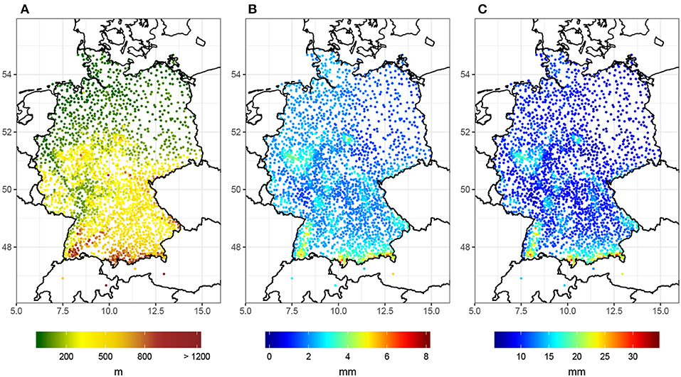
Figure 1. Location and basic properties of the stations forming the rain gauge network considered in this study: (A) altitude (in meters above mean sea level), (B) mean value, and (C) 95th percentile of daily rainfall sums (in mm).

Our data set is based on the same operational rain gauge network used in Zolina et al. (2008). However, their data set had over 200 stations less, and excluded Northeastern Germany entirely due to missing data and a lack of information about the applied measurement technique. Here, we close the information gap by using the post-processed product from the Potsdam Institute for Climate Impact Research (PIK).

The data set from PIK has the sole purpose of providing a complete and dense data basis for climate studies. The post-processing included a comprehensive quality control, a statistical replacement of missing values and the removal of inhomogeneities, if they were not of natural origin. Thus, the data set is complete and homogeneous for the entire time period between 1951 and 2006. All post-processing steps were carried out with careful consideration of statistical and climatological relationships between neighboring stations to ensure a physically robust temporal and spatial representation of precipitation events over Germany. As a detailed description of each individual post-processing step would exceed the scope of this article, we refer to Österle et al. (2006) for further information.

3. Methods

In this section, we give a short description of QR and the BM approach. For a more comprehensive introduction of QR and further details about its applications in various scientific disciplines (see Koenker, 2005). An equally comprehensive and well-written introduction of not only the block maxima approach but also the POT method can be found in Coles (2001). Additionally, a description of the likelihood ratio test is given.

All statistical methods used in this work and described below are available in the framework of existing packages in the open source statistical programming environment R (R Core Team, 2019). Specifically, the packages used include extRemes (Gilleland and Katz, 2016) for the block maxima approach, and quantreg (Koenker, 2019) for the quantile regression.

3.1. Block Maxima Approach

Let Y_t(t = 1, …, n) be a sequence of n independent and identically distributed random variables and M_n the respective BM

$\begin{array}{ll}{M}_n=max\left\{Y_1,\dots ,Y_n\right\}.& (1)\end{array}$

In extreme value statistics, M_n represents the most intense event in a block (i.e., time interval) of size n. In atmospheric science, n commonly covers a month or year. M_n would therefore be the magnitude of the most intense event in a month or year.

Following the extreme value theorem by Fisher and Tippett (1928), M_n converges for n → ∞ against one of three extreme value distributions (EVDs), i.e., Gumbel, Fréchet, or Weibull distribution. Each of these three EVDs represents a different type of PDF that exhibits a unique type of behavior in the tail. For the Gumbel distribution (Type I) the probability in the tail declines exponentially. The Fréchet distribution (Type II) is heavy-tailed, i.e., the PDF declines with a power law. The Weibull distribution (Type III), on the contrary, is light-tailed and the PDF has a finite upper endpoint.

The PDFs of the three EVDs can be generalized in terms of the generalized extreme value (GEV) distribution

$\begin{array}{ll}G(x;\mu ,\sigma ,\xi )=exp\left\{-{\left[1+\xi \left(\frac{x-\mu }{\sigma }\right)\right]}^{-1/\xi }\right\},& (2)\end{array}$

where μ ∈ ℝ is the location, σ > 0 the scale and ξ ∈ ℝ the shape parameter. The parameters describe different characteristics of the GEV. The location parameter μ determines the most likely magnitude of an extreme event, while σ represents the width of the density function. The shape parameter ξ is special as it not only describes the decline in the tail, but also links the GEV to the classical EVDs. In case of ξ > 0 the GEV corresponds to a Fréchet distribution, while ξ < 0 defines a Weibull distribution. The limit case ξ → 0 indicates a Gumbel distribution. A summary of the EVDs and their link to the GEV is provided in Table 1.

TABLE 1

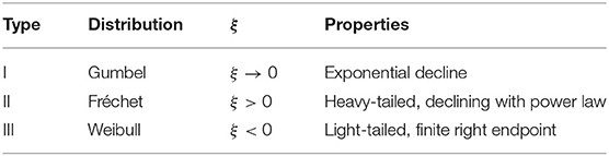
Table 1. Summary of the EDVs and their linking to GEV.

Because of the well-studied properties of the GEV distribution (Equation 2) and the intuitive definition of an extreme event as the most intense event in a given time interval (Equation 1), the block maxima approach has become a widely applied statistical tool not only in climatology and hydrology (Katz et al., 2002; Katz, 2010; Ribeiro et al., 2014), but also in economics (Embrechts and Schmidli, 1994) or engineering (Park and Sohn, 2006). However, as intuitive as the definition of M_n may be, the choice of block size (n) is the main challenge of the block maximum approach. If n is chosen too large, large sampling errors may occur due to the strong reduction of the data as only the maximum value of each block is used for the statistical inference. On the other hand, if n is chosen too small, estimation biases could occur due to a large number of unrepresentative local maxima. Therefore, a careful selection of n is important for every application of the block maxima approach.

Typically, n is chosen to fit the problem at hand, since the rate of convergence depends on the underlying distribution of Y_t (Embrechts and Schmidli, 1994). In past studies, 1-month blocks have proven proficient in representing the characteristics of heavy daily precipitation events in Europe (Rust et al., 2009; Fischer et al., 2018). Therefore, our study also uses monthly maxima for the estimation of the GEV parameters. The regression model for the parameters of the GEV is discussed in section 4.

3.2. Linear Quantile Regression

Let us again consider a sequence of n random variables Y_t(t = 1, …, n). For a desired probability τ the corresponding quantile Q_Yt(τ) is defined as

$\begin{array}{ll}{Q}_{Y_t}(\tau )=inf\left\{y:F_{Y_t}(y)\ge \tau \right\},& (3)\end{array}$

where τ ∈ [0, 1] and F_Yt is the cumulative distribution function (CDF) of Y_t. In Equation (3), the quantile is defined as stationary as long as F_Yt is stationary and can be interpreted as a threshold where the probability of an observation y being equal or below Q_Yt(τ) is τ. In linear QR, on the other hand, Q_Yt is defined as depending on a (t × p)-matrix of predictor variables X = (X₁₁, …, X_np) such that

$\begin{array}{ll}{Q}_{Y_t}(\tau |\text{X})=\text{X}·{\beta }_{\tau },& (4)\end{array}$

where β_τ = (β_{τ, 1}, …, β_{τ, p}) is a set of unknown regression parameters. Equation (4) describes a conditional quantile function (i.e., quantile values conditional on the set of predictors X), which serves a similar purpose as the conditional mean or expectation value in ordinary least square (OLS) regression (see Wood, 2006). In fact, QR can be seen as an extension of OLS regression. Analogous to the latter, Equation (4) is solved by minimizing a weighted sum of residuals

$\begin{array}{ll}{\widehat{\beta }}_{\tau }=\arg \underset{\beta \in {ℝ}^p}{\min }{\displaystyle \sum _{i=1}^n{\rho }_{\tau }}(Y_i-X_i·{\beta }_{\tau }),& (5)\end{array}$

where ρ_τ(·) is the tilted absolute value function

$\begin{array}{l}{\rho }_{\tau }(e)=\tau e{I}_{[0,\infty )}(e)-(1-\tau )e{I}_{(-\infty ,0)}(e)\\ =e(\tau -I_{(-\infty ,0)}(e))\\ =\left[\frac{1}{2}+\left(\tau -\frac{1}{2}\right)sgn(e)\right]|e|,& (6)\end{array}$

with sgn(·) being the sign function. The above linear quantile model can be generalized in a straightforward manner to also address non-linear functional forms of the quantiles' behavior by modifying the functional description in Equation (5) accordingly, in the same fashion as in OLS regression. Moreover, non-linear quantile trends can also be studied without prescribing a specific functional form of dependency by using different non-parametric (or semiparametric) versions of QR (see Donner et al., 2012, for a corresponding example).

By making use of Equations (4)–(6) (along with the possible generalizations as described in the previous paragraph), QR is able to estimate the parameters of arbitrary non-stationary functional relationships (quantile curves) for each set of desired quantiles τ in dependence on any given set of predictors X. In the context of the time series analysis, QR can be understood as an analog to a simple OLS regression for a time-dependent quantile, e.g., changes in the 99th percentile of daily observation values in each year. However, it should be noted that QR has a number of advantages compared to such a simplified approach. Most importantly, linear OLS regression for the 99th percentile of a year would reduce the data to one value per year. By contrast, QR estimates the trend coefficient of the linearly time-dependent 99th percentile using the whole time series (i.e., taking each individual observation value into account). This ensures a potentially more robust result for the estimated linear quantile trends.

3.3. Likelihood Ratio Test

In most applications of parametric regression, it is not necessarily evident whether or not a selected regression model is the most adequate to describe the problem at hand. In such cases, model selection approaches are commonly used to provide a degree of certainty about the selected regression model, i.e., the feasibility of a null model M₀, by testing it against one or more alternative model. Depending on the test statistic, M₀ is either rejected or not for a given significance level α.

One of the most flexible model selection tests is the likelihood-ratio test (LRT), a parametric test which compares the likelihood of two regression models. The test can be used in a straightforward manner if two conditions are satisfied. First, both regression models are nested such that M₀ with Θ = (θ₁, …, θ_j) is a simplification of M₁ with Θ = (θ₁, …, θ_k), where j < k. Hence, M₀ can be obtained by setting one or more parameters in M₁ to zero. Second, the parameters have been fitted using the method of maximum likelihood (see Wilks, 2011).

The null hypothesis of the LRT is that M₀ is a valid simplification of M₁ and will only be rejected if the likelihood associated with M₁ is sufficiently larger than that of M₀. The test statistic is

$\begin{array}{ll}D=2log\left[\frac{L(M_1)}{L(M_0)}\right]=2\left[logL(M_1)-logL(M_0)\right],& (7)\end{array}$

where L is the likelihood of the respective regression model. Equation (7) defines the so-called deviance statistic. Under the null hypothesis, and given a large sample size, the deviance's distribution resembles a χ² distribution with k − j degrees of freedom. Therefore, M₀ is rejected if the empirical value of D is in an improbable region of the tail of the χ² distribution defined by the residual error probability α.

We note that extensions of the LRT exist that work under more general conditions, i.e., cases in which the competing regression models are either nested, non-nested, or overlapping (e.g., Vuong, 1989). Such generalizations pose additional computational challenges, but would allow comparing regression models with unrelated predictors. However, since in this study all considered models are mutually nested, we will consider only the original LRT in the remainder of this work.

4. Model Selection

In this section, the above introduced LRT (section 3.3) is used to evaluate our regression models for QR and the block maxima approach. Both statistical methods will have the same regression models. Therefore, this section has two purposes. First, and most obviously, the selection of the most adequate regression model for this study. Second, to test whether both methods identify the same signals (i.e., significant parameters) in the observation data. The only major difference between QR and GEV will be that the same regression model may be applied to more than one parameter of the GEV, while in QR only one regression model is used for all probability levels.

Assuming a linear trend and annual cycle in the distribution of monthly maxima of daily precipitation, the parameters of the GEV are described as follows:

$\begin{array}{ll}\mu (t)={\mu }_0+{\mu }_{1}t+{\mu }_{2}sin(\omega c_i)+{\mu }_{3}cos(\omega c_i),& (8)\end{array}$

$\begin{array}{ll}ln\sigma (t)={\sigma }_0+{\sigma }_{1}t+{\sigma }_{2}sin(\omega c_i)+{\sigma }_{3}cos(\omega c_i),& (9)\end{array}$

$\begin{array}{ll}\xi (t)=\xi ,& (10)\end{array}$

where ω = 2π/365.25 is the angular frequency and c_i = c_i(t) the center of the i-th month in counted days beginning from the start of each year. The methodology and terminology were adapted from Rust et al. (2009) and, for the purpose of this application, extended by a linear trend component. The shape parameter is left stationary, as it is often difficult to estimate the parameter due to a lack of information in the tails of the distributions. Analogously, the regression model for QR will be

$\begin{array}{ll}{q}_{\tau }={\beta }_0+{\beta }_{1}t+{\beta }_{2}sin(\omega c_i)+{\beta }_{3}cos(\omega c_i),& (11)\end{array}$

where q_τ is the quantile value for the probability level τ.

To verify whether or not there is a significant trend in the fitted GEV parameters, four different settings will be tested against each other:

M₁: No trend at all (μ₁ = 0, σ₁ = 0)

M₂: Trend only in the location parameter (μ₁ ≠ 0, σ₁ = 0)

M₃: Trend only in the scale parameter (μ₁ = 0, σ₁ ≠ 0)

M₄: Trend in the location and scale parameter (μ₁ ≠ 0, σ₁ ≠ 0).

For QR, we will only test for β₁ ≠ 0 against β₁ = 0. All LRTs will be executed at a confidence level of α = 0.05. Note that in all configurations the annual cycle will be part of the regression. This is because we want to explain as much natural variability within the data as possible while estimating the trends.

We note that in general, long-term trends in climatological variables are not necessarily linear, but often mutually entangled with low-frequency variability, making the “slow” changes (i.e., on time scales of the order of the observation period) in fact non-linear. Despite this, we have to acknowledge this fact, as we restrict ourselves to linear time dependencies here for two main reasons: First, linear trends can be characterized by a single coefficient (i.e., the slope), which can be interpreted in a very intuitive way. Specifically, non-linear trends imply that the rate of changes becomes itself time-dependent, which needs to be accounted for in the interpretation. Second, we attempt a comparative study between temporal changes in GEV parameters and conditional quantiles of the distribution of daily precipitation values. Since the employed extreme value statistics makes use of block maxima, using more complex than linear behaviors (in addition to the modeled seasonality) as parts of the corresponding modeling problem is likely to render the resulting parameter estimates more uncertain and, therefore less interpretable. Recalling that a statistical model should be as complex as necessary, but not more complex, we will exclusively study the aforementioned linear model versions in this work.

Figure 2 shows the resulting p-values for the comparison of all configurations. For the BM approach, most stations in Germany show no significant trends in heavy precipitation events. When there is a significant trend, then it is usually found in the location parameter of the GEV (Figure 2A). For the scale parameter there are close to no significant trends (Figure 2B). This suggests that the intensity distribution of heavy precipitation events rather tends to shift to higher or lower intensities while the overall variance remains about the same. There is no visible improvement when both parameters include a linear trend as compared to a GEV model where only the location parameter has a linear trend (Figure 2C).

FIGURE 2

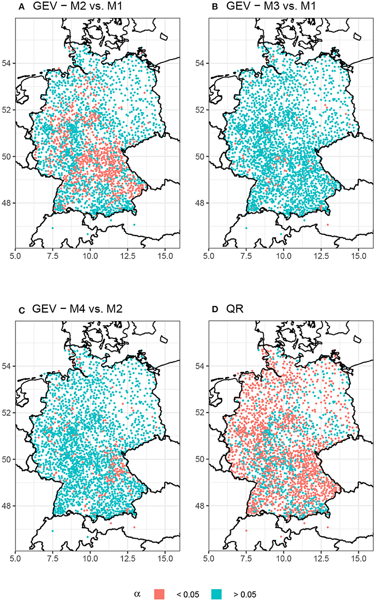
Figure 2. Resulting p-values from the LRT for (A–C) different configurations of the GEV (M₁-M₄) and (D) QR for 95th percentile (β₁ ≠ 0 vs. β₁ = 0). A trend is considered significant for p ≤ 0.05.

Notably, significant trends in the location parameter (Figure 2A) mostly occur at stations in Central, Southeast, Southwest and higher altitude regions of Western Germany. More than half of these stations are located at least 300 m above sea level (cf. Figure 1). There are only a few significant trends in Northern Germany and almost none in Eastern Germany.

Figure 2D shows the resulting p-values for QR with τ = 0.95. Most stations in Germany show a significant trend in the 95th percentile. In accordance with Figure 2A, there are particularly large clusters of significant trends in Southeastern and Central Germany. Differences can be seen for Western, Northwestern and Eastern Germany. Here, the 95th percentile exhibits significant trends for a majority of the stations. Other percentiles between 90 and 99% show similar results when tested under the same conditions (not shown).

Based on the results in Figure 2 and considering the purpose of this article, the remainder of our analysis will focus on the GEV model where only the location parameter is modeled with a linear trend (M₁) along with the QR model with β₁ ≠ 0 for all desired percentiles.

5. Results

5.1. Comparison of QR and the Block Maxima Approach

Because of their distinct methodological foundations, the BM approach and QR do not have much in common conceptually. However, both methods are able to represent statistical characteristics of the tails of a given distribution. Therefore, it is meaningful to investigate the relationship between the fitted location parameter of the GEV and the upper quantiles of the precipitation distribution.

Figure 3 shows two scatter plots for the intercepts and trend coefficients, respectively. There is a high correlation between the intercepts (μ₀ and β₀) for all upper quantiles (Figure 3A). For the 95th percentile, μ₀ and β₀ are almost equal. Note, that there is no physical interpretation for the intercept. In a regression model, the intercept is the expected mean value of the response variable if the predictor equals zero. Here, in a case were the predictor is never zero, the intercept has no intrinsic meaning and is fully dependent on the data. For the given data and regression models, our block maxima approach and the QR estimate of the 95th percentile estimates similar intercepts. One could interpret this as both approaches using similar starting values for their regression.

FIGURE 3

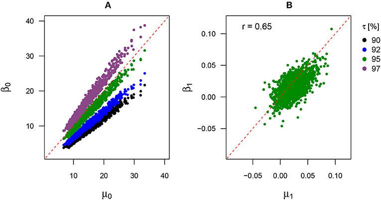
Figure 3. Scatter plots for the relationship between the location parameter of the GEV and QR for (A) the respective intercepts (μ₀, β₀) and (B) the respective trend coefficients (μ₁, β₁) with associated Person correlation coefficient (r). The intercepts are compared for different τ.

Based on the results in Figure 3A, only the comparison of the respective trend coefficients for the GEV location parameter and 95th percentile is shown in Figure 3B. The estimated β₁ and μ₁ show a medium high correlation of r ≈ 0.65. All estimates are located close to the diagonal line, implying μ₁ ≈ β₁. Since the scatter cloud is slightly shifted toward the right side of the plot, μ₁ seems to have larger values overall than β₁. However, the respective parameter estimates of both methods do not always perfectly coincide, which is expected since the mean amplitude of monthly block maxima (representing about 12/365.25 or 3.3% of all daily observations) and the 95th percentile of the full distribution of the daily data constitute two closely related yet different statistical properties.

5.2. Trends in Precipitation Extremes

To quantify the magnitude and spatial distribution of trends in the intensity of heavy precipitation events, Figure 4 shows the maps of β₁ and μ₁ over Germany. The trends are categorized from large positive trends to large negative trends. We do this for two reasons; (i) a categorization simplifies the visualization of spatial patterns and (ii) it filters small differences between β₁ and μ₁, which are solely based on the different methodologies of QR and GEV, or small variance in the respective estimators.

FIGURE 4

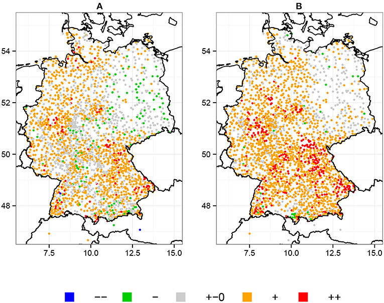
Figure 4. Trends in the intensity of heavy precipitation over Germany. Trends are categorized into large positive trend (++, x > 0.04 mm/yr), small positive trend (+, x > 0.01 mm/yr), nearly no change (+–0, –0.01 mm/yr < x < 0.01 mm/yr), small negative trend (–, x < –0.01 mm/yr), or large negative trend (–, x < –0.04 mm/yr), where x is a place holder for (A) β₁ and (B) μ₁.

Figure 4 shows that most regions in Germany have experienced an increase in the intensity of heavy precipitation for the period between 1951 and 2006. Trends are generally stronger in the BM than in the 95th percentile. The spatial distribution, however, is similar for both β₁ and μ₁. The regions with the strongest increases in intensity are Southeastern and Central Germany. In both regions, the majority of β₁ and μ₁ are considered to be significant (cf. Figure 2). Most of the large positive trends in Figure 4 can be associated with stations about 300 m above sea level and in close approximation too even higher altitude regions (cf. Figure 1). This suggests an increasing role of orographic lifting in heavy precipitation events. However, the majority of stations display only a small increase in intensity of heavy precipitation.

Overall, the block maxima approach and QR show a consistent picture for trends in the intensity of heavy precipitation events. An exception to this is Northeastern Germany, where the patterns are more distinct between both methods. Here, μ₁ shows no clear trends in heavy precipitation, while β₁ suggests an overall decrease in intensity. Similarities apply to the Alpine Foreland, where almost all block maxima exhibit positive trends, whereas the trends in the 95th percentile either indicate no changes or a decrease in intensity. In both regions, Figure 2 shows almost no significant trends in μ and only a few in β. In such cases of disagreement, we suggest exploring both methods in parallel instead of taking one as a reference, since (as stated above) both are based on different rationales and thereby capture related, yet different aspects of a time-dependent probability distribution.

5.3. Trends in Precipitation Quantiles

One of the advantages of QR compared to the block maxima approach is its ability to provide a more comprehensive understanding of the PDF's behavior because it is not limited to a particular definition of an extreme event. To give an example, we selected 10 stations from different regions in Germany (Figure 5) and estimated the linear trends in various quantiles. Figure 6 shows the resulting quantile trends for probabilities from 0.6 to 0.98 (henceforth denoted as trend curves). Associated uncertainties were estimated using the inverted rank test for dependent data as proposed by Koenker and Machado (1999).

FIGURE 5

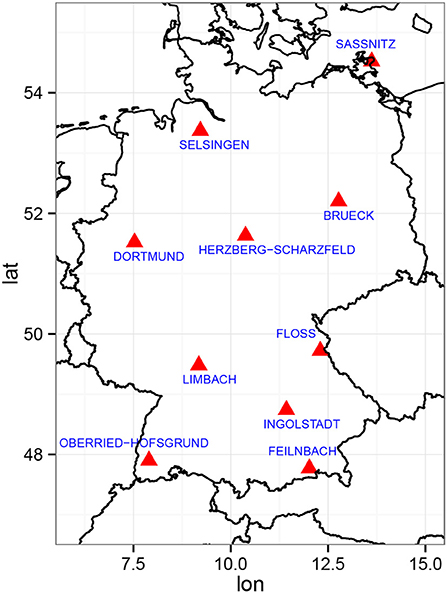
Figure 5. Location and names of the 10 example stations.

FIGURE 6

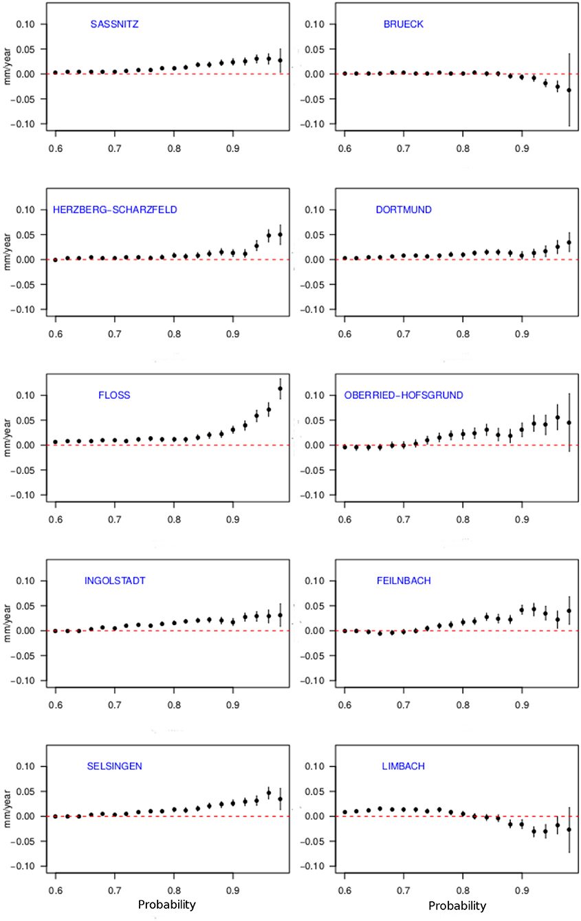
Figure 6. Estimated quantile trends and corresponding uncertainties (vertical error bars) for probabilities τ ≥ 0.6 at 10 different stations in Germany. The uncertainty was calculated using a maximum entropy bootstrap algorithm.

Generally, the strongest quantile trends can be seen in the upper quantiles (above τ > 0.8) of the distribution. Here, most of the stations show an increase in intensity. Only the stations Brück and Limbach display negative trends over the observation period. Surprisingly, none of the stations shows a continuous transition between quantile trends. However, there seem to be similar patterns in the transition. From Figure 6, four different categories can be identified. First, a slow increase of the trend curve with a drop at the 0.98 quantile (Figure 6, Sassnitz and Selsingen). Second, almost no response below the most extreme quantiles (Figure 6, Dortmund and Herzberg-Scharzfeld). Third, strong positive quantile trends for almost all probabilities (Figure 6, Feilnbach, Oberried-Hofsgrund, Ingolstadt and Floss). Fourth and last, a decreasing trend curve in the upper quantiles (Figure 6, Brueck and Limbach).

The uncertainty of the estimate increases together with the probability level. This is to be expected, since although QR makes use of the full data, independent of the desired τ, the weighting function (Equation 6) still increases the impact of a smaller number of values on the estimate as τ reaches the tails. For example, consider the estimation of the 99th percentile. In such a case, the majority of the residuals would get a weighting of 0.01, while only few residuals would be weighted with 0.99. Hence, the minimization process (Equation 5) would be mostly governed by just 1% of the data.

Figure 6 suggest a regional pattern of trend curves, since the stations within the above identified categories are usually from the same region. For example, the stations Sassnitz and Selsingen are both located in the northern part of Germany. To further study the corresponding pattern, we use k-means clustering for the obtained linear QR trend curves as a function of the percentile all stations in Germany using Lloyd's algorithm (Lloyd, 1982). Here, k initial cluster means are estimated by randomly choosing k out of all available stations (initialization step). Each individual station is assigned to the cluster who's mean QR trend curve has the least squared Euclidean distance to that of the respective station (assignment step). Afterwards, new means are estimated depending on the cluster variance (update step). The assignment and update step are repeated until the algorithm converges, i.e., the assignments of stations to different clusters no longer change. The final mean QR trend curves of all stations belonging to the same cluster are called the centers of those clusters. A more comprehensive description of Lloyd's algorithm can be found in Lloyd (1982).

A drawback of k-means clustering is that the number of clusters k has to be prescribed prior to the application of the algorithm. If there is no a priori knowledge about the possible number of clusters within the data, k must be chosen based on empirical reasoning. There are various statistical approaches to the assessment of clustering quality that can be used for determining an appropriate k, ranging from simple visual methods to more complex measures for cluster comparison. Here, we use the average silhouette method proposed by Rousseeuw (1987), which provides a quantitative way to measure how well each point lies within its cluster in comparison to the other clusters. Both, the average silhouette method and Lloyd's algorithm, are available in the R package NbClust (Charrad et al., 2014).

To find an optimal number of clusters among all stations based on the similarity between the quantile curves, the average silhouette method is applied to different ensembles of clusters, where each ensemble consists of 50 k-means clustered members all evaluated with the same k. In our case, the number of clusters k varies between 2 and 6. Therefore, silhouette values are calculated for 5 ensembles of 50 k-means members each. The ensemble with the on average highest silhouette value is the ensemble with the optimal k. We use ensembles to account for the variance in cluster assignments originating from the initialization step in Lloyd's algorithm, because the random picking of stations as initial means can lead to somewhat different clustering each time the algorithm is applied, which needs to be considered when choosing between different k. The results of the above described methodology (not shown) suggest that k = 2 is the optimal number of clusters for our problem according to the average silhouette criterion.

The cluster centers for k = 2 and the respective cluster assignments of all stations are shown in Figure 7. The resulting clusters are nearly balanced, with group 1 consisting of 1,071 stations and group 2 of 1,271 stations. Both cluster centers display only positive trends in all quantiles (Figure 7, lower panel). The quantile curves in group 1 exhibit positive trends, which strongly increase toward the upper quantiles. The quantile curves of stations in group 2, on the other hand, show only weak positive trends, which display a rather slow and continuous increase toward the uppermost quantiles. Stations with negative trends like Limbach (see Figure 6) are assigned to group 2, suggesting that stations with negative or decreasing trends in the upper quantiles are too rare to justify individual clusters in the considered version of the k-means approach. Indeed, when allowing for a larger number of clusters k, the diversity of behaviors markedly increases and qualitatively matches the empirical observations made based upon Figure 6 (not shown).

FIGURE 7

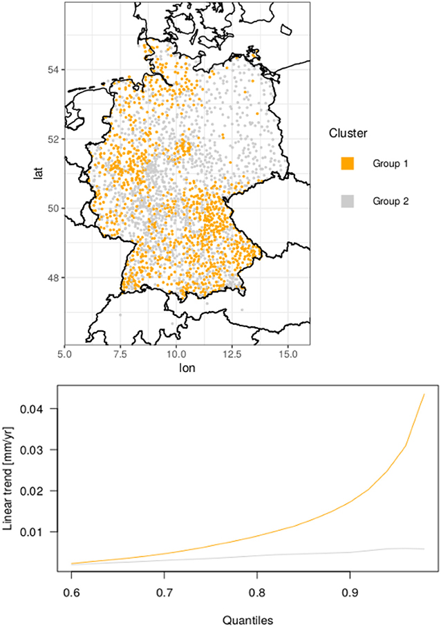
Figure 7. Resulting k-means clusters (Upper) with corresponding centers (Lower) represented by the mean QR trend curves for quantiles from 0.6 to 0.98. The color of each group applies to both panels.

The spatial distribution of the two clusters (Figure 7, upper panel) supports the results in Figures 4A,D. Stations with strong positive trends in the upper quantiles (group 1) usually cluster westwards of high orography (Central and Southeast Germany) or in the northwestern region near the North Sea, while the northeastern part of Germany is mostly caused by stations with only weakly positive or even negative trends (group 2) in the upper quantiles.

6. Discussion and Conclusion

In this article, we proposed QR as a complementary and powerful statistical tool for EVS. QR's proficiency was shown by a statistical assessment of recent trends in the intensity spectrum of heavy precipitation over Germany based on a spatially and temporally high-resolution data set covering the period from 1951 to 2006. To verify the methodological consistency of QR in the context of EVS, an additional well-established method from extreme value theory was applied—the BM approach. While QR estimates quantile curves from data in a fashion similar to OLS, the BM approach aims to approximate the GEV for a set of given BM.

Although both methods follow a different philosophy, a high correlation between the location parameter of the GEV and the 95th percentile estimated by QR could be found. This high correlation and the similar results from sections 5.2 and 5.3 show the methodological consistency of both methods and support the statement that, when applied together, a more comprehensive and complete understanding is achieved. Two regions with large clusters of significant trends were identified by both QR and the BM approach, one in Central and another in Southeastern Germany. Both regions exhibit the strongest overall trends for the period 1951–2006. Additionally, QR identified a significant increase in the 95th percentile for large parts of Germany. In the test statistics for QR, however, we compared a regression model consisting of a parameterization of the annual cycle with the same regression model plus a linear trend. A simple parameterization of the annual cycle might be insufficient to effectively describe the underlying data, which is why the inclusion of a linear trend could already significantly improve the regression model and thus cause the LRT indicating too many significant trends. However, stations for which both QR and the BM approach produce significant trends are likely to have experienced a change in the intensity of heavy precipitation events.

The strongest trends with a significant increase in intensity can be found at stations with an altitude of 300 m above sea level or more. These results suggest an increasing role of orography in the intensity of heavy precipitation. This hypothesis is further supported by the fact that the majority of negative trends were found in the northeastern part of Germany, a region with an average altitude of about 100 m above sea level and less, or in a mountain lee. Here, however, only a few of stations showed a significant trend in both QR and the BM approach. Furthermore, a k-means clustering analysis of quantile trend curves showed that the upper percentiles (80th percentile and above) usually experience stronger trends than those below.

The mainly positive trends in the northwestern part of Germany could be governed by the North Atlantic oscillation (NAO) through an increased import of moist air in the winter periods. The NAO is a major source of interannual variability in the atmospheric circulation and influences the surface westerlies across the North Atlantic onto Europe (Rogers, 1985). Its positive mode is highly correlated to precipitation in North and Northwest Germany, especially in winter (Cleary et al., 2017). Hurrell (1995) found that the NAO shows an increased tendency toward the positive mode since 1980. Hence, an upward trend in the occurrence probability of positive NAO modes would be directly linked to increasing trends in winter precipitation.

In summary, the results suggest that positive trends in the intensity of heavy precipitation could be associated to regional characteristics such as high elevation and orography or moisture transport from adjoining large water bodies. This increasing role of regional effects on precipitation could be indirectly related to the aerosol effect on cloud droplet size. The cloud droplet size is found to be smallest in polluted air masses over the continent (Bréon et al., 2002). Clouds consisting of too many small cloud droplets, however, are less likely to produce raindrops due to coalescence, leaving longer-lived clouds (the so-called “cloud lifetime hypotheses,” see Albrecht, 1989). A characteristic of these clouds could be that they need a trigger to initiate other precipitation formation processes such as the Wegener-Bergeron-Findeisen process (Findeisen, 2015). Such a trigger could be regional effects like orographic lifting. In the context of climate change, this could mean that future extreme events become increasingly related to regional characteristics due to increasing emissions of aerosols from anthropogenic sources.

However, pinpointing direct or even indirect causes for such trends is hardly justifiable within the scope of the presented assessment, since we only analyze daily precipitation amounts without consideration of related climate variables such as temperature, wind or pressure. Further investigation is needed to provide physical robust explanations of changes in heavy precipitation and its causes.

As a final note, we emphasize that our results indicate a spatial dependency of heavy precipitation trends in Germany. Therefore, it might be reasonable to explicitly account for this dependency in future investigations of climatic changes. Especially in the context of regression approaches, including parameters for altitude and location of the event which could further improve the models, thereby leading to a better understanding of regional precipitation characteristics. The potential of such a regression model was already evaluated in Fischer et al. (2017). Here, the authors introduced spatially and seasonally varying parameters into a GEV distribution fitted on monthly maxima of daily precipitation sums using Legendre polynomials for spatial characteristics (i.e., longitude, latitude, and altitude) and harmonic functions for seasonality. Their results showed a significant improvement in model accuracy, as the inclusion of time and location dependent parameters allowed the GEV to be applied to the entire data set instead of each month and station separately. For future investigations, it would thus be interesting to see if such a similar strategy of spatial modeling could also further improve the performance of our quantile regression approach.

Author Contributions

All authors listed have made a substantial, direct and intellectual contribution to the work, and approved it for publication.

Funding

This work has been financially supported by the German Federal Ministry for Education and Research via the Young Investigators Group CoSy-CC² (Complex Systems Approaches to Understanding Causes and Consequences of Past, Present, and Future Climate Change, Grant No. 01Ln1306A) and the Belmont Forum/JPI Climate project GOTHAM (Globally Observed Teleconnections and their Representation in Hierarchies of Atmospheric Models, Grant No. 01LP16MA). We also acknowledge support by the German Research Foundation and the Open Access Publication Fund of the Freie Universität Berlin.

Conflict of Interest

The authors declare that the research was conducted in the absence of any commercial or financial relationships that could be construed as a potential conflict of interest.

References

Albrecht, B. A. (1989). Aerosols, cloud microphysics, and fractional cloudiness. Science 245, 1227–1230. doi: 10.1126/science.245.4923.1227

PubMed Abstract | CrossRef Full Text | Google Scholar

Alexander, L. V., Zhang, X., Peterson, T. C., Caesar, J., Gleason, B., Klein Tank, A. M. G., et al. (2006). Global observed changes in daily climate extremes of temperature and precipitation. J. Geophys. Res. Atmos. 111:D05109. doi: 10.1029/2005JD006290

CrossRef Full Text | Google Scholar

Austin, P. C., Tu, J. V., Daly, P. A., and Alter, D. A. (2005). The use of quantile regression in health care research: a case study examining gender differences in the timeliness of thrombolytic therapy. Stat. Med. 24, 791–816. doi: 10.1002/sim.1851

PubMed Abstract | CrossRef Full Text | Google Scholar

Barbosa, S. M. (2008). Quantile trends in baltic sea level. Geophys. Res. Lett. 35:L22704. doi: 10.1029/2008GL035182

CrossRef Full Text | Google Scholar

Barbosa, S. M., Scotto, M. G., and Alonso, A. M. (2011). Summarising changes in air temperature over central europe by quantile regression and clustering. Nat. Hazards Earth Syst. Sci. 11, 3227–3233. doi: 10.5194/nhess-11-3227-2011

CrossRef Full Text | Google Scholar

Bréon, F.-M., Tanré, D., and Generoso, S. (2002). Aerosol effect on cloud droplet size monitored from satellite. Science 295, 834–838. doi: 10.1126/science.1066434

PubMed Abstract | CrossRef Full Text | Google Scholar

Charrad, M., Ghazzali, N., Boiteau, V., and Niknafs, A. (2014). NbClust: an R package for determining the relevant number of clusters in a data set. J. Stat. Softw. 61, 1–36. doi: 10.18637/jss.v061.i06

CrossRef Full Text | Google Scholar

Cleary, D. M., Wynn, J. G., Ionita, M., Forray, F. L., and Onac, B. P. (2017). Evidence of long-term NAO influence on East-Central Europe winter precipitation from a guano-derived δ15N record. Sci. Rep. 7:14095. doi: 10.1038/s41598-017-14488-5

PubMed Abstract | CrossRef Full Text | Google Scholar

Coad, A., and Rao, R. (2008). Innovation and firm growth in high-tech sectors: a quantile regression approach. Res. Policy 37, 633–648. doi: 10.1016/j.respol.2008.01.003

CrossRef Full Text | Google Scholar

Coles, S. (2001). An Introduction to Statistical Modeling of Extreme Values. Springer Series in Statistics. London: Springer.

Google Scholar

Ding, R., McCarthy, M. L., Desmond, J. S., Lee, J. S., Aronsky, D., and Zeger, S. L. (2010). Characterizing waiting room time, treatment time, and boarding time in the emergency department using quantile regression. Acad. Emerg. Med. 17, 813–823. doi: 10.1111/j.1553-2712.2010.00812.x

PubMed Abstract | CrossRef Full Text | Google Scholar

Donner, R. V., Ehrcke, R., Barbosa, S. M., Wagner, J., Donges, J. F., and Kurths, J. (2012). Spatial patterns of linear and nonparametric long-term trends in Baltic sea-level variability. Nonlinear Process. Geophys. 19, 95–111. doi: 10.5194/npg-19-95-2012

CrossRef Full Text | Google Scholar

Elsner, J. B., Kossin, J. P., and Jagger, T. H. (2008). The increasing intensity of the strongest tropical cyclones. Nature 455, 92–95. doi: 10.1038/nature07234

PubMed Abstract | CrossRef Full Text | Google Scholar

Embrechts, P., and Schmidli, H. (1994). Modelling of extremal events in insurance and finance. Z. Oper. Res. 39, 1–34. doi: 10.1007/BF01440733

CrossRef Full Text | Google Scholar

Findeisen, W. (2015). Colloidal meteorological processes in the formation of precipitation (translated and edited by E. Volken, A.M. Giesche, S. Brönnimann). Meteorol. Z. 24, 443–454. doi: 10.1127/metz/2015/0675

CrossRef Full Text | Google Scholar

Fischer, M., Rust, H., and Ulbrich, U. (2017). A spatial and seasonal climatology of extreme precipitation return-levels: a case study. Spatial Stat. doi: 10.1016/j.spasta.2017.11.007. [Epub ahead of print].

CrossRef Full Text | Google Scholar

Fischer, M., Rust, H. W., and Ulbrich, U. (2018). Seasonal cycle in German daily precipitation extremes. Meteorol. Z. 27, 3–13. doi: 10.1127/metz/2017/0845

CrossRef Full Text | Google Scholar

Fisher, R. A., and Tippett, L. H. C. (1928). Limiting forms of the frequency distribution of the largest or smallest member of a sample. Math. Proc. Camb. Philos. Soc. 24, 180–190.

Google Scholar

Gao, M., and Franzke, C. L. E. (2017). Quantile regression-based spatiotemporal analysis of extreme temperature change in china. J. Clim. 30, 9897–9914. doi: 10.1175/JCLI-D-17-0356.1

CrossRef Full Text | Google Scholar

Gilleland, E., and Katz, R. W. (2016). extRemes 2.0: an extreme value analysis package in R. J. Stat. Softw. 72, 1–39. doi: 10.18637/jss.v072.i08

CrossRef Full Text | Google Scholar

Hartmann, D., Tank, A. K., Rusticucci, M., Alexander, L., Bönnimann, S., Charabi, Y., et al. (2013). “Climate change 2013: the physical science basis, Chapter Observations: Atmosphere and Surface,” in Contribution of Working Group I to the Fifth Assessment Report of the Intergovernmental Panel on Climate Change, eds T. F. Stocker, D. Qin, G.-K. Plattner, M. Tignor, S. K. Allen, J. Boschung, A. Nauels, Y. Xia, V. Bex, and P. M. Midgley (Cambridge; New York, NY: Cambridge University Press), 213–216.

Google Scholar

Haugen, M. A., Stein, M. L., Moyer, E. J., and Sriver, R. L. (2018). Estimating changes in temperature distributions in a large ensemble of climate simulations using quantile regression. J. Clim. 31, 8573–8588. doi: 10.1175/JCLI-D-17-0782.1

CrossRef Full Text | Google Scholar

Huber, P. J., and Ronchetti, E. M. (2009). “Chapter Generalities,” in Robust Statistics, eds D. J. Balding, N. A. C. Cressie, G. M. Fitzmaurice, I. M. Johnstone, G. Molenberghs, D. W. Scott, A. F. M. Smith, R. S. Tsay, and S. Weisberg (Hoboken, NJ: John Wiley & Sons, Ltd.), 1–21.

Google Scholar

Hurrell, J. W. (1995). Decadal trends in the North Atlantic oscillation: regional temperatures and precipitation. Science 269, 676–679.

PubMed Abstract | Google Scholar

IPCC (2012). “Chapter Summary for Policymakers,” in Managing the Risks of Extreme Events and Disasters to Advance Climate Change Adaptation. A Special Report of Working Groups I and II of the Intergovernmental Panel on Climate Change (Cambridge; New York, NY: Cambridge University Press), 3–21.

Google Scholar

John, O. O. (2015). Robustness of quantile regression to outliers. Am. J. Appl. Math. Stat. 3, 86–88. doi: 10.12691/ajams-3-2-8

CrossRef Full Text | Google Scholar

Katz, R. W. (2010). Statistics of extremes in climate change. Clim. Change 100, 71–76. doi: 10.1007/s10584-010-9834-5

CrossRef Full Text | Google Scholar

Katz, R. W., Parlange, M. B., and Naveau, P. (2002). Statistics of extremes in hydrology. Adv. Water Resour. 25, 1287–1304. doi: 10.1016/S0309-1708(02)00056-8

CrossRef Full Text | Google Scholar

Klein Tank, A. M. G., and Können, G. P. (2003). Trends in indices of daily temperature and precipitation extremes in europe, 1946–99. J. Clim. 16, 3665–3680. doi: 10.1175/1520-0442(2003)016<3665:TIIODT>2.0.CO;2

CrossRef Full Text | Google Scholar

Koenker, R. (2005). Quantile Regression. Econometric Society Monographs. Cambridge: Cambridge University Press.

PubMed Abstract | Google Scholar

Koenker, R. (2019). Quantreg: Quantile Regression. R package version 5.41.

Google Scholar

Koenker, R., and Bassett, G. (1978). Regression quantiles. Econometrica 46, 33–50. doi: 10.2307/1913643

CrossRef Full Text | Google Scholar

Koenker, R., and Geling, O. (2001). Reappraising medfly longevity. J. Am. Stat. Assoc. 96, 458–468. doi: 10.1198/016214501753168172

CrossRef Full Text | Google Scholar

Koenker, R., and Machado, J. A. F. (1999). Goodness of fit and related inference processes for quantile regression. J. Am. Stat. Assoc. 94, 1296–1310.

Google Scholar

Lloyd, S. (1982). Least squares quantization in PCM. IEEE Trans. Inform. Theor. 28, 129–137.

Google Scholar

Machado, J. A. F., and Mata, J. (2005). Counterfactual decomposition of changes in wage distributions using quantile regression. J. Appl. Econometr. 20, 445–465. doi: 10.1002/jae.788

CrossRef Full Text | Google Scholar

Österle, H., Gerstengarbe, F., and Werner, P. (2006). “Qualitätsprüfung, Ergänzung und Homogenisierung der täglichen Datenreihen in Deutschland, 1951–2003: Ein neuer Datenansatz,” in Proceedings der 7 Deutschen Klimatagung Klimatrends: Vergangenheit und Zukunft (Munich).

Google Scholar

Park, H. W., and Sohn, H. (2006). Parameter estimation of the generalized extreme value distribution for structural health monitoring. Probab. Eng. Mech. 21, 366–376. doi: 10.1016/j.probengmech.2005.11.009

CrossRef Full Text | Google Scholar

Peng, L., and Huang, Y. (2008). Survival analysis with quantile regression models. J. Am. Stat. Assoc. 103, 637–649. doi: 10.1198/016214508000000355

CrossRef Full Text | Google Scholar

R Core Team (2019). R: A Language and Environment for Statistical Computing. Vienna: R Foundation for Statistical Computing.

PubMed Abstract | Google Scholar

Rhines, A., McKinnon, K. A., Tingley, M. P., and Huybers, P. (2017). Seasonally resolved distributional trends of north american temperatures show contraction of winter variability. J. Clim. 30, 1139–1157. doi: 10.1175/JCLI-D-16-0363.1

CrossRef Full Text | Google Scholar

Ribeiro, A., Barbosa, S. M., Scotto, M. G., and Donner, R. V. (2014). Changes in extreme sea-levels in the Baltic Sea. Tellus A 66:20921. doi: 10.3402/tellusa.v66.20921

CrossRef Full Text | Google Scholar

Rogers, J. C. (1985). Atmospheric circulation changes associated with the warming over the Northern North Atlantic in the 1920s. J. Clim. Appl. Meteorol. 24, 1303–1310.

Google Scholar

Rousseeuw, P. J. (1987). Silhouettes: a graphical aid to the interpretation and validation of cluster analysis. J. Comput. Appl. Math. 20, 53–65.

Google Scholar

Rust, H. W., Maraun, D., and Osborn, T. J. (2009). Modelling seasonality in extreme precipitation. Eur. Phys. J. Spec. Top. 174, 99–111. doi: 10.1140/epjst/e2009-01093-7

CrossRef Full Text | Google Scholar

van den Besselaar, E. J. M., Klein Tank, A. M. G., and Buishand, T. A. (2013). Trends in European precipitation extremes over 1951–2010. Int. J. Climatol. 33, 2682–2689. doi: 10.1002/joc.3619

CrossRef Full Text | Google Scholar

Vuong, Q. H. (1989). Likelihood ratio tests for model selection and non-nested hypotheses. Econometrica 57, 307–333. doi: 10.2307/1912557

CrossRef Full Text | Google Scholar

Wasko, C., and Sharma, A. (2014). Quantile regression for investigating scaling of extreme precipitation with temperature. Water Resour. Res. 50, 3608–3614. doi: 10.1002/2013WR015194

CrossRef Full Text | Google Scholar

Wilks, D. S. (2011). Statistical Methods in the Atmospheric Sciences, 3rd Edn, Vol. 100. Oxford: Academic Press.

Google Scholar

Wood, S. N. (2006). “Chapter Linear Models,” in Generalized Additive Models: An Introduction with R, 1st Edn, eds B. P. Carlin, C. Chatfield, M. Tanner, and J. Zidek (New York, NY: Chapman and Hall/CRC), 1–54.

Google Scholar

Zolina, O., Simmer, C., Kapala, A., Bachner, S., Gulev, S., and Maechel, H. (2008). Seasonally dependent changes of precipitation extremes over Germany since 1950 from a very dense observational network. J. Geophys. Res. Atmos. 113:D06110. doi: 10.1029/2007JD008393

CrossRef Full Text | Google Scholar