Inversion Algorithm for Civil Flood Defense Optimization: Application to Two-Dimensional Numerical Model of the Garonne River in France

1. Introduction

It is well-known that the world's major lowland rivers (the Rhine, the Po, the Elbe River, and the Loire River) are protected against flooding by embankments or other flood defenses (Ciullo et al., 2019). The embankments and so-called primary flood defenses such as flood walls and dams (Kind, 2014) are aimed primarily at reducing the likelihood of flooding in the protected area, and historically they have been the most commonly-adopted flood risk reduction measure (Ciullo et al., 2019). The design of these flood protection measures is therefore of major importance society-wide, and can have a considerable impact on the economic and demographic development of the alluvial plains (White, 1945).

The classical approach for flood defense systems design was developed in the Netherlands in the wake of the 1953 disaster (see Vrijling, 2001). Since, reliability-based flood defense design strategies have been developed all over the world (see Vrijling, 2001; van Gelder and Vrijling, 2004; Ciullo et al., 2019). These strategies mainly involve the statistical quantification of the hazard (see Vrijling, 2001; Apel et al., 2004; van Gelder and Vrijling, 2004; Polanco and Rice, 2014) and the “economic” optimization of the flood defense systems (see Vrijling, 2001; van Gelder and Vrijling, 2004; Ciullo et al., 2019). The optimum design is considered to be the value at which the total cost of investment (which increases with the height of the flood defense) and the present value of the risk (which diminishes with the increasing height) takes its minimum (see Vrijling, 2001; van Gelder and Vrijling, 2004; Ciullo et al., 2019). Another good example is the optimization model introduced by van Dantzig (1956) for the embankment height, which was further developed by other authors, as reported by Eijgenraam et al. (2016).

These statistical studies are well-suited to the definition of a global flood protection strategy (at “country” scale), as they are not supported by intensive numerical modeling. Although the value of these models is indisputable, the flooding probabilities of the protected areas are assumed to be independent of one another, disregarding the change in hydraulic load along the river stretch as a consequence of the state (e.g., failure, increase in safety) of the embankments elsewhere (Ciullo et al., 2019).

At a local scale, in practical engineering applications, the classical method for the design of flooding protections for urban and industrial facilities relies on the development of sophisticated and refined numerical model systems able to reproduce surface flow accurately for a given chosen “design scenario” (such as the 100-year return period flood event). The quantities of major interest for the design of a flood defense (wall, urban structures, drainage network, etc.) are often related to the parameters describing this design scenario, such as the water height at a given location, or the water velocity in the inundated area (Milanesi et al., 2015). Once these quantities are evaluated, the flood defense is accordingly designed.

Although robust, this “classical approach” can appear too simplified considering the variability of natural phenomena and the numerous uncertainties related to natural hazard modeling. Ideally, flood disaster mitigation strategies should be based on a comprehensive assessment of the flood risk, combined with a thorough investigation of the uncertainties associated with the risk assessment procedure (Apel et al., 2004). Specifically, numerous studies have demonstrated the influence of uncertainties on flood hazard assessment (see Apel et al., 2004; Alho and Mäkinen, 2010; Domeneghetti et al., 2013; Maurizio et al., 2014; Nguyen et al., 2015; Abily et al., 2016; Bacchi et al., 2018), sometimes underling the hard-to-estimate damage caused by flooding (see Apel et al., 2004). These studies are often based on the use of simplified numerical models which reduce the computational time (see Apel et al., 2004; Alho and Mäkinen, 2010; Domeneghetti et al., 2013; Maurizio et al., 2014; Nguyen et al., 2015), and they are an example of how uncertainty quantification techniques could be employed for the assessment of natural hazards. If applied to the design of flood defenses, these studies can be considered an “improvement” on the classical approach, since they make it possible to better evaluate the uncertainties related to the “design” parameters, which in this case are the target values derived from uncertainty quantification (i.e., a target water height).

However, both the “classical” and “improved” approach for flood defense design suffer the same limitations, as they do not allow the end-user of the methodology to robustly evaluate the best flood defense configuration (the geometry) for the natural variability of the simulated phenomenon. Within this context, the objective of this work is therefore to investigate the “robust inversion approach,” subsequently referred to as RSUR, for the design of a flood defense in a two-dimensional inundated area. This method consists in defining a “safety criterion” (such as “the water level in the slab must remain lower than 25 cm”) and the analysis of suitable design parameters (for instance, the elevation of the flood defenses) that ensure the safety objective for all the possible combinations of uncertain input parameters (for instance, the flow hydrograph characteristics) describing the natural phenomenon to be met.

To estimate this safety set, a standard surrogate approach will be used (Jones et al., 1998), which significantly reduces the number of model evaluations needed. This algorithm relies on a kriging surrogate built from a few model evaluations, sequentially enriched with new numerical model evaluations as long as the remaining uncertainty of the entire safety set remains too high (Chevalier, 2013). This algorithm therefore appears well-suited to the rigorous study of the uncertainties of very refined numerical models traditionally used in engineering applications. Belonging to a more general class of “Stepwise Uncertainty Reduction,” this algorithm is embedded in the “Prométhée” workbench (using the “Funz” engine) tasked with bridging the numerical model and any design of experiments algorithm (further technical information is provided in an Annex).

In this research work, we first introduce the engineering problem we want to solve (section 2). Our proposed methodology for model resolution is then presented (section 3) with a focus on the numerical tools we develop for the methodology's application to the chosen real case (section 4). Lastly, the results and main conclusions and perspectives are reported (section 5). The results will be introduced as the safety set and will be analyzed in terms of safety control within the river's operating range. Once properly evaluated, this constrained zone provides highly valuable data for full risk-informed management of the river.

2. Problem Specification

The study area is a 50-km-long reach on the Garonne river between Tonneins and La Réole (Figure 1). The area was settled to protect flood plains by organizing flooding and flood storage between 1760 and 1850, when many earthen levees were built to protect the harvest against spring floods (LPCB, 1983; SMEPAG, 1989). The river was canalized to protect residents from flooding after the historic 1875 flood event (SMEPAG, 1989).

FIGURE 1

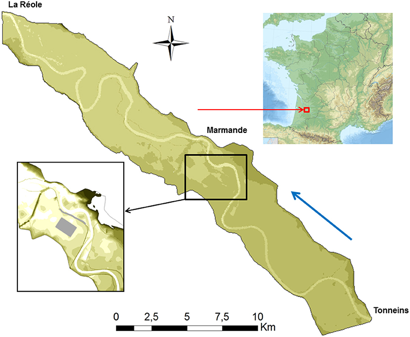
Figure 1. Location and span of the modeled study area on the Garonne river including the location of the industrial site (gray surface) and the protection (gray line) requiring modification to meet the safety criterion.

In this section of the Garonne river, the flood defense is actually designed for a river flood of nearly 3,500 m³/s. Specifically, successive storage areas give the Garonne profiles a particular configuration and allow flooding in the floodplain to be controlled. Figure 2 shows three flow characteristics on a typical cross-section of the Garonne to illustrate the flooding sequence: (1) base flow 1,100 m³/s; (2) bankfull flow 2,400 m³/s; and (3) flow before overflow of the levees with the lowest protection level 3,500 m³/s. Consequently, flooding of the less protected areas between Tonneins and La Réole occurs with a low return period, i.e.,~10 years, and only a few levees have a standard of protection higher than 30 years. Due to the flat topography and the presence of a steep floodplain lateral slope, the floodplains are largely inundated even for high-probability floods. The December 1981 flood was one of the largest floods occurring since the most severe flood on record (1875); this flood event was used as a reference for our study. During this 9-day event, the peak discharge measured at Tonneins reached 6,040 m³/s, corresponding approximately to a 20-year flood, and the floodplains were fully inundated.

FIGURE 2

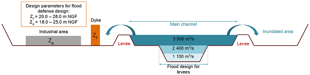
Figure 2. Typical cross-section of the Garonne between Tonneins and La Réole and the design zone. In gray, the industrial area (slab elevation Z_a), in orange, the wall to be designed (elevation Z_f).

Within this context, it was decided to site an industrial area spanning nearly 1 km² in the vicinity of the left bank of the Garonne river (see gray area in Figure 1). This zone is protected by a dyke that is nearly 2 km long, 20 m wide and at a constant elevation of nearly 25.8 m NGF¹ (see gray line in Figure 1). However, the local topography of this zone varies between 18 and 22 m NGF, and the area is fully inundated during a flooding event characterized by a peak discharge higher than 3,500 m³/s according to the current design of the dykes (see Figure 2). To protect the new industrial area against flooding, a decision was made to investigate the impact of modifying the current crest of the dyke and the basement of the future industrial area.

More practically, the objective of the study is to identify the actual dyke elevation and the platform elevation (the slab), to ensure the industrial area remains operational under all possible watershed flooding exceeding the defense (occurring at nearly 3,500 m³/s). Specifically, the water height in the vicinity of the industrial area must not exceed 0.25 m above the slab, which is the safety criterion of this study. With this aim, we made the following assumptions for the uncontrolled input parameters (the flow hydrograph) and the controlled input parameters (crest of the flood defense, basement of the industrial area), both of which have a different role in the RSUR algorithm workflow presented in Table 1 below:

TABLE 1

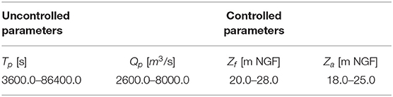
Table 1. Qualified parameters of the study: time to peak discharge T_p, peak discharge rate Q_p, dyke elevation Z_f, slab elevation Z_a.

The methodology used and the numerical chain developed for the study are presented in the next sections.

3. Methodology for Robust Design of Protections

The intrinsic nature of many engineering problems like flooding protection is a combination of several “canonical” problems (a word used to express a natural orthogonality), mainly within the following mathematical classes:

• Optimization (e.g., search for the worst flood conditions).

• Inversion (e.g., set defense to not exceed 25 cm of flooding).

• Randomization (e.g., integrate a probabilistic flooding model according to a given model like the Gumbel law).

For instance, here we choose to describe the flood protection problem as a combination of designing protections to avoid exceeding a given water level (i.e., inversion part) when faced with the worst rain conditions for a given return period (i.e., max/optimization part). It should be noted that qualification of these aspects of the problem is somewhat arbitrary and may largely depend on the country's regulation practice and the safety objective considered.

However, regardless of the choice made, the main nature of the problem considered (the identification/inversion of a flood level) is often “tainted” by secondary issues (worst flooding conditions), and all the parameters belong to one of these canonical roles. As an example, we could also mention other common engineering problems like robust optimization (optimizing some parameters and considering others as random) or constraint optimization (optimizing some parameters, keeping others verifying an [in]equality).

This “real-world” engineering practice also brings more complexity than canonical problems and thus requires dedicated algorithms in order to be solved efficiently (Chevalier, 2013). In the following, we will focus on the “robust inversion” problem, where the objective is to restore the civil engineering safety set identified for the worst flooding conditions without any probabilistic assumption.

3.1. Bayesian Metamodeling

The fairly common practice of Bayesian metamodeling is now a standard for solving any engineering task requiring numerous CPU-expensive simulations. Indeed, since the seminal paper describing the Efficient Global Optimization (EGO) algorithm (Jones et al., 1998; Roustant et al., 2012), many improvements have been proposed, investigating the algorithms' efficiency (Picheny and Ginsbourger, 2013) or different problems to solve (Chevalier et al., 2014).

The rationale behind this approach consists in replacing most of the costly numerical simulations with an inexpensive surrogate function to investigate the properties that are relevant to our engineering purpose, like possible optimizers, excursion set or its main parameter effects. This surrogate function is designed to interpolate a few known “true” simulation points (Figure 3), taken as conditioning events of an initial uncertain/random function. Starting with a largely uncertain metamodel (Figure 3), this iterated process leads to a very precise metamodel around “true” simulated points, cleverly chosen in relation to our engineering objective (Figure 3):

FIGURE 3

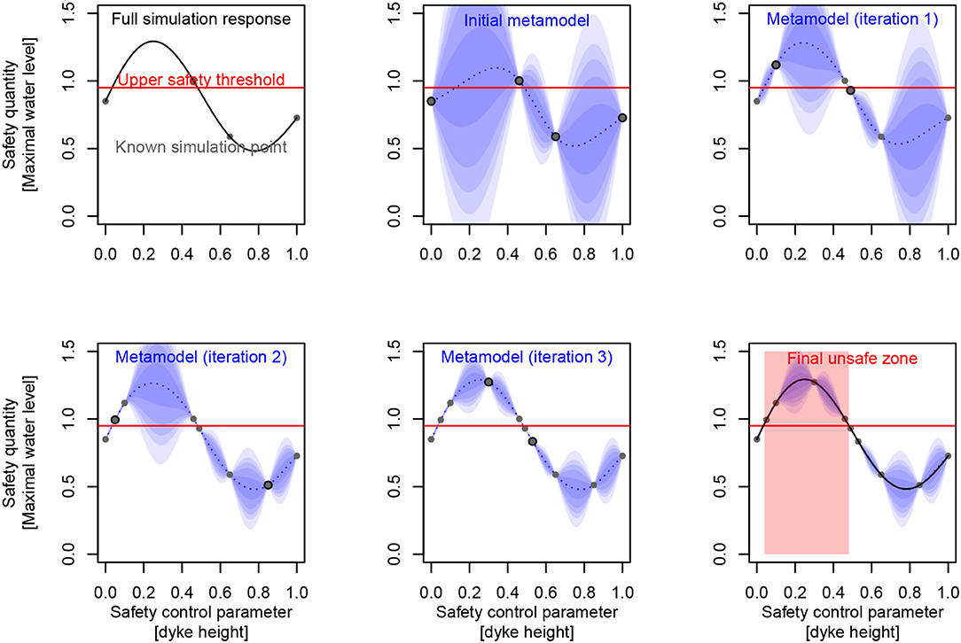
Figure 3. (Left to right, top to bottom) Identification of a safety set on a synthetic case, based on a kriging metamodel iteratively filled/conditioned to reduce set uncertainty (the dots are detailed simulations performed).

A variety of metamodels have been applied in the water resources literature (Santana-Quintero et al., 2010; Razavi et al., 2012). Moreover, some examples of applications in the context of flood management have already been published (e.g., Yazdi and Salehi Neyshabouri, 2014; Löwe et al., 2018). However, like the previously mentioned EGO algorithm, for the study presented here, we will rely on conditional Gaussian processes (also known as kriging Roustant et al., 2012), derived from Danie Krige's pioneering work in mining, later formalized within the geostatistical framework by Matheron (1973). Our choice is mainly motivated by this non-parametric metamodeling because although some properties of the considered response surface may be assumed (like continuity, derivability, etc.), its precise shape cannot be assumed a priori. Thus, kriging became a standard metamodeling method in operational research (Santner et al., 2003; Kleijnen, 2015) and has performed robustly in previous water resource applications (Razavi et al., 2012; Villa-Vialaneix et al., 2012; Löwe et al., 2018). More practically, it is of considerable interest when investigating engineering objectives like max-minima or level sets of such random functions, inheriting convenient properties of Gaussian processes, and the method is fast provided the datasets exceed no more than a few hundred observations. The kriging model (which later provides an estimation of water height in an industrial area) is then defined for x ∈ S (x will then represent study variables like the slab and dyke height or flow hydrograph parameters) as in the following Gaussian process:

$\begin{array}{ll}M(x)={N}(m(x),s^2(x))& (1)\end{array}$

where (for “simple” kriging):

• {X, Y} are the coordinates of the “true” numerical simulations, taken as conditioning events of the statistical process:

• thus conditional mean is m(x) = C(x)^TC(X)⁻¹Y

• thus conditional variance is s²(x) = c(x) − C(x)^TC(X)⁻¹C(x)

• C is the covariance kernel C(.) = Cov(X, .), c(.) = Cov(x, .)

More than a commonplace deterministic interpolation method (like splines of any order), this model is much more informative owing to its predicted expectation and uncertainty. The fitting procedure of this model includes the choice of a covariance model [here a tensor product of the “Matern5₂” function, (Roustant et al., 2012)], and then the covariance parameters (e.g., range of covariance for each input variable, variance of the random process, nugget effect, etc.), could be estimated using Maximum Likelihood Estimation (standard choice we made) or Leave-One-Out minimization [known to mitigate the arbitrary covariance function choice (see Bachoc, 2013)], or even sampled within a full Bayesian framework (too far from our computational constraints at present). Once such a metamodel is specified, the following criteria will draw on such information to optimize the algorithm's iterative sampling policy.

3.2. Design of (Numerical) Experiments

Once the Bayesian metamodeling framework is provided, the remaining issue is to define the sampling criterion used to fill the design of experiments: each batch of experiments will be proposed by the algorithm, then evaluated by the numerical simulator, and returned to the algorithm in order to propose the next batch (Algorithm 1). This general iterative process must be defined for each problem addressed: X input space, Y output target, and J criterion of interest (see later canonical or hybrid concrete instantiations):

ALGORITHM 1

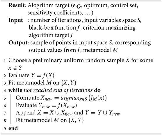
Algorithm 1: Sequential design of numerical experiments procedure based on J criterion of interest

Improvements to this fully sequential procedure have been proposed, like asynchronization (Le Riche et al., 2012) which may reduce the servers' sleep time between iterations (especially if the simulations have very different computing times). Nevertheless, it is often easier to consider synchronous batching (Ginsbourger et al., 2010) as an efficient turn-around to reduce user time, so the algorithm we will actually use becomes (Algorithm 2):

ALGORITHM 2

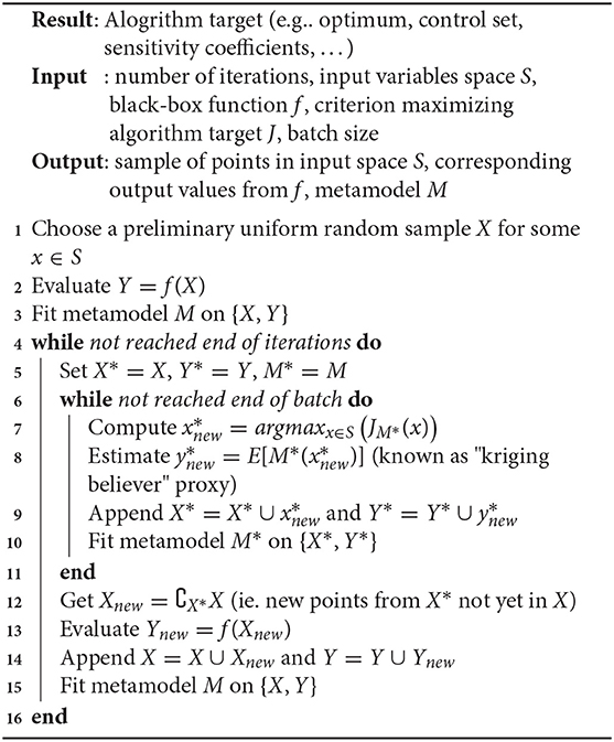
Algorithm 2: Batch sequential design of numerical experiments procedure based on J criterion of interest

Note that this last algorithm may be greatly improved and likened to the previous one, when the criterion J is computable (in closed form) for a whole batch of points (see Chevalier and Ginsbourger, 2013 for such optimization criterion), which is sadly not often the case.

3.2.1. Canonical Optimization Problem

The EGO algorithm (Jones et al., 1998) is the common entry point for batch sequential kriging algorithms, as it proposes an efficient criterion (standing for criterion of interest J) called the “Expected Improvement” (EI):

$\begin{array}{ll}J:x\to EI(x)=E\left[{(min(Y)-M(x))}^{+}\right]& (2)\end{array}$

• . → .⁺ being “positive part” function,

• M is the kriging metamodel (see Equation 1),

• X is the optimization input space,

• Y are the black-box function evaluations on X (see Equation 1).

Computing this criteria (using the previous kriging formulas) is quite simple, so the main issue relates to the optimization of this criterion, whose maximum will define the most “promising” point for the next batch. This strategy will just propose the next point, and although a “multiple expected improvement” criterion (Chevalier and Ginsbourger, 2013) allows many points to be proposed at a time, it remains practically more robust (numerically speaking) to use heuristics, which are usually preferred by practitioners: “Constant Liar,” “Kriging Believer” (see Picheny and Ginsbourger, 2013).

3.2.2. Canonical Inversion Problem

Beyond such criteria dedicated to optimization problems, others are proposed to solve the (also) canonical problem of inversion, like Bichon's criterion (Bichon et al., 2008) which is similar to Expected Improvement, but focuses on proposing points closest to the inversion target:

$\begin{array}{ll}J:x\to EE(x)=E\left[{(s(x)-|T-M(x)|)}^{+}\right]& (3)\end{array}$

• . → .⁺ being “positive part” function,

• M is the kriging metamodel and s its variance (see Equation 1),

• X belongs to the inversion input space S,

• T being the target value of inversion output Y.

Other criteria for inversion have been proposed (Ranjan et al., 2008), but all of these so-called “punctual” criteria have the same intrinsic limitation of searching for a punctual solution to the inversion problem, while the answer should lie in a non-discrete space (usually a union of subsets of S).

Trying to solve the inversion problem more consistently will require defining an intermediate value like the uncertainty of the excursion set above (or below) the inversion target (Bect et al., 2012). A suitable criterion will then focus on decreasing this value, and the final inversion set will be identified through the metamodel instead of its sampling points. This leads to the “Stepwise Uncertainty Reduction” (SUR) family of criteria (also abusively naming the following inversion algorithm) which takes a non-closed form, unlike the previous punctual ones:

$\begin{array}{l}J:x\to SUR(x)\\ =-E\left[{\displaystyle {\int }_{S}P}[T<M_{n+\left\{x\right\}}(x^{\prime })]\times P[T\ge M_{n+\left\{x\right\}}(x^{\prime })]d{x}^{\prime }\right]\\ =-E\left[{\displaystyle {\int }_{S}P}[T<M_{n+\left\{x\right\}}(x^{\prime })]\times (1-P[T<M_{n+\left\{x\right\}}(x^{\prime })])d{x}^{\prime }\right]& (4)\end{array}$

• M_n+{x} is the kriging metamodel conditioned by the n points {X, Y} (just like “M” in Equation 1), plus the new point x,

• X belongs to the inversion input space S,

• T is the target value of inversion output Y,

• so $P\left[T<M_{n+\left\{x\right\}}(x^{\prime })\right]$ stands for the probability of exceedance in x′, then $P\left[T<M_{n+\left\{x\right\}}(x^{\prime })\right]\times (1-P\left[T<M_{n+\left\{x\right\}}(x^{\prime })\right])$ gives a null contribution in the integral as far as $M_{n+\left\{x\right\}}(x^{\prime })$ is certainly upper or lower than T.

At the cost of a significantly more computer-intensive task, the SUR criterion will propose more informative points and avoid the over-clustering defect often encountered with “punctual” criteria (even with the EGO algorithm whose exploration/exploitation trade-off is indeed due to heuristic tuning).

3.2.3. Robust Inversion Hybrid Problem

A by-product of the SUR algorithm is the extensive formulation used, which allows a flexible expression of the interest expectation. Therefore, it is now possible to use more complex interest values, for instance relying on the process properties of each subspace: S_c for controlled parameters and S_u for uncontrolled parameters. The “Robust Inversion” will then use the statistic of the marginal uncontrolled maximum (on S_u) of the process to integrate into the criterion (Chevalier, 2013):

$\begin{array}{l}J:x\to RSUR(x=\{x_c,x_u\})\\ =-E_n\left[{\displaystyle {\int }_{S_c}{P}_{n+1}}({x^{\prime }}_c)\times (1-P_{n+1}({x^{\prime }}_c))d{x^{\prime }}_c\right]& (5)\end{array}$

where:

• x = {x_c, x_u}:**

– x_c stands for the coordinate of x in the input controlled subspace S_c,

– x_u stands for the coordinate of x in the input uncontrolled subspace S_u,

• P_n+1(x_c) = P[T < max_xu∈Su(M_{n+{xc, xu}}(x_c, x_u))] is the marginal uncontrolled maximum probability:

– M_n+{x} is the kriging metamodel conditioned by the n points {X, Y} (just like “M”), plus the new point x,

– T being the target value of inversion.

Using such an expression combines non-homogeneous subspaces, here an inversion subspace (for controlled variables) S_c, and an optimization subspace (for uncontrolled variables) S_u. Thus, this criterion leads to a hybrid algorithm of optimization “inside” inversion. More generally, this approach may be used to establish other criteria to solve hybrid problems. For instance, just replacing the “max_xu” statistic (used to define P_n+1(x_c)) by a mean or quantile on S_u may be useful for solving a probabilistic inversion problem, instead of the present worst-case inversion. Such hybrid algorithms are often much closer to solving real engineering concerns than purely canonical algorithms.

At this point of reasoning, it is very important to understand that a one-point marginal prediction of any kriging model is not sufficient to fully access the process behavior (and thus integrate it). Indeed, the correlation function behind process C(., .) is strongly related to the process sample functional properties, which may vary greatly depending on the kernel assumption (Figure 4). Such a process statistic (maximum here) is then impossible to compute as an independent sum of punctual evaluations of x ∈ S. A simple, but more costly approach consists in using a simulation of the random processes instead of its prediction statistical model.

FIGURE 4

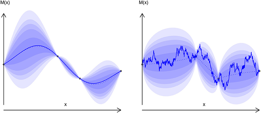
Figure 4. Exponential (right) and gauss (left) kernels random processes. Plain line: one sample drawing, dotted line: mean value, blurred zone: quantiles.

Using this latter criterion (Equation 5) on our practical case study, we will now ask the algorithm (Algorithm 2) to sample the S space, trying to identify the safety set (dyke and slab height), irrespective of the flooding duration and discharge values.

In a self-supporting form, the batch sequential algorithm using this RSUR criterion on a TELEMAC-2D model of the Garonne river becomes:

4. Software and Numerical Tools

This work lies within a trend of applied research aimed at engineering enhancement. In practice, the previous (Algorithm 3) requires a heterogeneous set of hardware and software to be applied. The workbench which drives the simulations according to the algorithm: (Richet, 2019) [which may also be used through its Graphical User Interface (Richet, 2011)] is intended to fill the gap between:

• the flooding simulations: TELEMAC-2D, running in parallel on some Amazon Web Services “instances” (i.e., virtual machines);

• the robust inversion algorithm: RSUR, from the RobustInv R package (Chevalier et al., 2017). As a “reproducible research” target, these components are all available as free software and standard hardware (see Annex for details of how to implement them on a cloud platform).

ALGORITHM 3

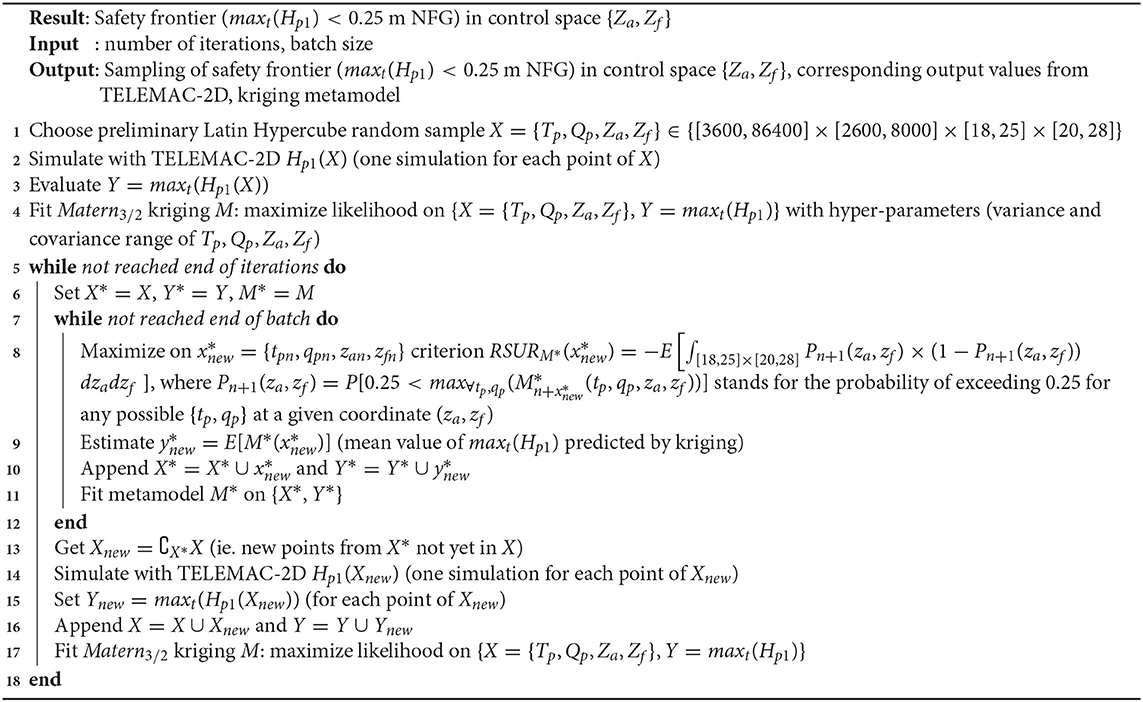
Algorithm 3: Batch sequential procedure to sample the safety frontier (max_t(H_p1) < 0.25 m NFG) in control space {Z_a, Z_f}

4.1. Hydrodynamic Model of the Study Area

The Institut de radioprotection et de sûreté nucléaire (Institute for Radiological Protection and Nuclear Safety, IRSN) has been involved in the “Garonne Benchmark” project instigated by EDF. The aim of the project was to obtain an uncertainty quantification with hydraulic modeling on a stretch of the Garonne river. Earlier work carried out by Besnard and Goutal (2011) and Bozzi et al. (2015), has investigated discharge and roughness uncertainty in 1D and 2D hydraulic models. In order to contribute to the project, a version of the MASCARET 1D and TELEMAC-2D model, as well as hydraulic and hydrological data required to build these numerical models, were provided to the project's participants. In Besnard and Goutal (2011), the models' capacities to represent a major flood event were compared.

In this study, we use 2D model TELEMAC-2D from the open TELEMAC-MASCARET system (http://www.opentelemac.org). TELEMAC-2D solves 2D depth-averaged equations (i.e., shallow water Equation 6). Disregarding the Coriolis, wind and viscous forces and assuming a vertically hydrostatic pressure distribution and incompressible flow, the 2D depth-averaged dynamic wave equations for open-channel flows can be written in conservative and vector form as:

$\begin{array}{ll}\partial U/\partial t+\nabla ·F=S& (6)\end{array}$

where

• t = time (seconds)

• (x, y, z) = coordinate system with the x-axis longitudinal, y-axis transversal and the z-axis vertical upward (meters)

• U = [h, hu, hv]^T = vector of conservative variables, with h being flow depth (meters), u and v = x and y-components of the velocity vector (meters/seconds)

• F = F(U) = [E(U), G(U)] = flux vector with E = [hu, hu² + gh²/2, huv]T and G = [hv, huv, hv² + gh²/2]T (g is gravitational acceleration in meters/seconds²)

• S = S₀ + S_f, with $S_0={\left[0,-gh\partial z_b/\partial x,-gh\partial z_b/\partial y\right]}^T$ = dimensionless bottom slope and $S_f={\left[0,-g{n}^{2}u{(u^2+v^2)}^{1/2}/h^{1/3},-g{n}^{2}v{(u^2+v^2)}^{1/2}/h^{1/3}\right]}^T$ = energy losses due to the bottom and wall shear stress, where z_b is bed elevation and n is Manning roughness (seconds/meters^1/3).

The roughness is flow and sediment dependent, but for simplicity it is assumed to be constant in each of the numerical runs. In this work, turbulence is modeled using a constant eddy viscosity value.

A two-dimensional model of the study area was constructed by EDF within the framework of the “Garonne Benchmark” (Besnard and Goutal, 2011). The model is composed of nearly 82,116 triangular elements with different lengths varying from 10 m (for the dyke crest, or the main channel of the Garonne River) to 300 m for the inundated areas. The floodplain topography and bathymetry are represented by the interpolation of the triangular mesh on the photogrammetry data (downstream part of the study area) and the national topographic map (upstream part). The model covers nearly 136 km² of the Garonne river basin. It is forced upstream (the “Tonneins” section) by a flow hydrograph and downstream by considering steady flow conditions (the “La Réole” section). The model calibration is reported in Besnard and Goutal (2011).

The presented model was modified slightly in this study to introduce the industrial area reported in Figures 1, 2. The industrial platform was inserted into the model by elevating the topography of the corresponding mesh at a constant mean level varying from 18.0 to 25.0 m NGF (Table 1).

For the purpose of the study, triangular flow hydrographs were used in the upstream section of the model. At the beginning of each simulation, a steady flow corresponding to a permanent discharge of 2,100 m²/s is imposed on the model. The flow discharge is then increased linearly until the maximum water discharge (Q_p) is reached at the time step corresponding to T_p. Once the peak discharge Q_p is reached, the discharge is decreased linearly until the permanent flow of 2,100 m³/s is reached at a time step of 2 * T_p.

4.2. Robust Inversion Algorithm

The Robust Stepwise Uncertainty Reduction (RSUR) algorithm was implemented in a dedicated R package (Chevalier et al., 2017). It should be used in the same way as other R packages dedicated to Bayesian optimization or inversion like DiceOptim (Picheny and Ginsbourger, 2013) or KrigInv (Chevalier et al., 2012). However, for convenient and simple integration (in the Funz workbench), the standardized wrapper of the MASCOT-NUM research group (Monod et al., 2019) was applied to provide a front API² (http://www.gdr-mascotnum.fr/template.html) with the following R functions (https://github.com/Funz/algorithm-RSUR):

• RSUR(options): basic algorithm constructor, will return RSUR object to hold algorithm state

• getInitialDesign(rsur,input,output): function to return a first random sample based on input and output information (dimension, bounds, etc.)

• getNextDesign(rsur,X,Y): function to return iterative new samples which maximize the RSUR criterion, based on previous {X, Y} conditions

• displayResults(rsur,X,Y): function to display the current state of the RSUR algorithm based on previous {X, Y} conditions.

4.3. Funz Workbench

Developed by the IRSN and distributed under the BSD³ license (https://github.com/Funz), Funz is a server client engine designed to support parametric scientific simulations. An overhanging graphical user interface design for practical engineering is also available at http://promethee.irsn.fr. Funz can be easily and quickly linked to any computer simulation code through a set of wrapping expressions (a set of regexp-like lines in the ASCII file). It uses the R programming language that is freely available and widely used by the scientific community working with applied mathematics. In addition to its use by the research community, this language is also used by many regulatory organizations. It is therefore simple to integrate algorithms developed and validated by the scientific community into Funz, which can then be applied to the previously-linked computer codes. Thus, to perform this study, Funz was used to link Telemac (plugin available at https://gtihub.com/Funz/plugin-Telemac) and the RSUR algorithm (available at https://github.com/Funz/algorithm-RSUR).

Moreover, in order to perform a given set of computations, Funz can bring together independent servers, clusters (above their own queue manager if available), workstations, virtual servers (see Annex for Amazon Web Services / EC2 example), and even desktop computers running Windows, MacOS, Linux, Solaris, or other operating systems. While more focused on medium-sized performance computing (usually less than 100 concurrent connected instances), the high performance bottleneck is indeed delegated to each connected simulator instance, able to require dozens of CPUs independently (or even launch a Funz master itself).

5. Results, Analysis, and Conclusions

5.1. Overview Results of Algorithm

As previously mentioned, the RSUR algorithm is parameterized with:

• Controlled parameters: Z_a ∈ [18, 25] (slab elevation), Z_f ∈ [20, 28] (dyke elevation),

• Uncontrolled parameters: T_p ∈ [3600, 86400] (time to peak), Q_p ∈ [2600, 8000] (peak discharge rate),

• Objective function: max_t(H_p1) < 0.25 (p1 being one point in the center of the slab, this means we aim to not exceed 25 cm of water on this slab),

• Batches of 8 calculations at each iteration (plus 2⁴ calculations of input parameter boundary combinations).

• 20 iterations of (algorithm 2).

Among these, the computing parameters (20 batches of 8 simulations) are defined arbitrarily, considering that:

• the number of iterations (20) has to be increased with the number of variables, so that the relative uncertainty of the control set reaches some percent in the end;

• the batch size (8) is mainly an opportunistic choice related to our computing resources, but it is also an empirical equilibrium to limit the batching effect of the 8 simultaneous points chosen [to mitigate the temporary hypothesis effect in M^*, see (Algorithm 2)].

The convergence of the algorithm is measured by the remaining uncertainty on the control set volume (numerically, this is the opposite of the RSUR criterion value (see Chevalier et al., 2014 for computing details) in Figure 5. This quantifies the “fuzzy zone” where it is still unclear whether the safety limit is exceeded or not, or in other words, where the limit is exceeded with a probability which is not 0 or 1 (visually the “gray zone”, while the “white zone” contains definite unsafe points, and the “black zone” definite safe points, Figure 6).

FIGURE 5

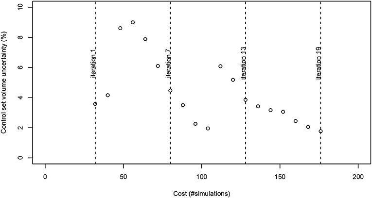
Figure 5. Convergence of RSUR criterion during iterations.

FIGURE 6

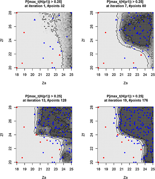
Figure 6. Probability of exceeding the level of 25 cm on the slab, depending on the controlled Z_a and Z_f parameters, along some RSUR iterations (last added points as triangles, exceeding the points in red). The fairly dense sampling of the “safe” zone represents a practical safety guarantee.

It should be noted that some intermediate raising of the RSUR criterion occurs (e.g., between iterations 10 and 11), when the kriging metamodel is changing abruptly because of the last data acquired, thus correcting the fitting of some kriging parameters. Between iterations 10 and 11, the range of covariance over the Z_f variable decreases (from 9.1 to 7.43), so the algorithm expects a lower regularity on the Z_f dimension, which leads us to “discover” an unexpected safe zone for Z_a > 24 & Z_f < 23.

The safety-controlled set S_c = {Z_a, Z_c} is iteratively identified, with increasing accuracy along the iterations (Figure 6):

It should be noted that the sampling density of the three zones is intrinsically different because of the asymmetry of the algorithm concerning the property of “unsafety”:

• The assumed “safe” zone needs to be sampled densely to assume its true safety ⁴.

• The “unsafe” zone is discovered with sparse sampling, as just one exceeding (of level set) point is sufficient.

• The frontier between safe/unsafe is explored very densely, it being the critical information returned by the algorithm.

In addition to this raw result on the S_c subspace, it is also useful to consider some specific coordinates in their S_u projection. The response surface interpolated (by the kriging mean predictor) on such interest points, whose side of the frontier may lead to the safety criterion being exceeded (Figures 7–9) (max_t(H_p1) > 0.25 are red points):

• Definitely “unsafe”: exceeding max_t(H_p1) > 0.25, for (Z_a, Z_f) in the unsafe zone:

• On the frontier: max_t(H_p1) ~ 0.25, for (Z_a, Z_f) in the undefined safety zone:

• Almost definitely “safe”: max_t(H_p1) < 0.25, for (Z_a, Z_f) taken in the safe zone:

FIGURE 7

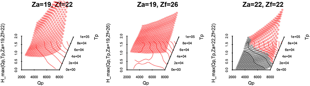
Figure 7. Metamodel mean response surface on S_u for surely unsafe points.

FIGURE 8

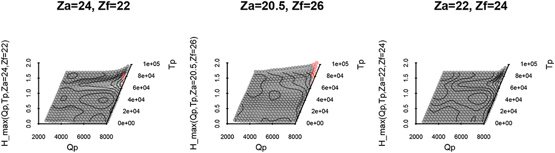
Figure 8. Metamodel mean response surface on S_u for safety limit points.

FIGURE 9

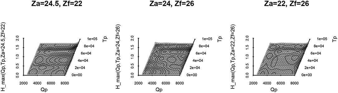
Figure 9. Metamodel mean response surface on S_u for surely safe points.

It should be noted that it was quite expected that maximum duration and discharge would be observed as the most penalizing configuration of this study, which is confirmed by these projections. When such an assumption may be proven prior to a study, it should be reached by using just an SUR algorithm, reducing the optimization space to a known value: S_u = {T_p, Q_p} = {max(T_p), max(Q_p)}.

5.2. Validation of Results

Validation of the previous results [i.e., the accuracy of the safe/unsafe limit where max_t(H_p1) ≃ 0.25] should be performed considering the accuracy of the kriging metamodel obtained at the end of the algorithm iterations. Nevertheless, it is sufficient to verify that the metamodel is sufficiently accurate for max_t(H_p1) ≤ 0.25, as the inaccuracy of the metamodel for higher values where max_t(H_p1) >> 0.25 has no crippling impact on safety.

The best possible measurements of metamodel inaccuracy should be obtained using a fully-independent test basis of points, which is unattainable in most practical cases, where financial and resource constraints prevail. A cheaper alternative lies in cross-validation inaccuracy estimators, keeping in mind that this estimate is a “proxy” of the metamodel prediction error (see Bachoc, 2013). We will use the standard “Leave-One-Out” (LOO) estimator which computes the Gaussian prediction at each design point x_i ∈ X when x_i is artificially removed to re-build the kriging metamodel (see Equation 7):

$\begin{array}{ll}{y}_{-i}=M_{n-\left\{x_i\right\}}={N}(m_{-i}(x),s_{-i}^2(x))& (7)\end{array}$

Where M_n−{xi} is the kriging metamodel conditioned by the n points {X, Y} (just like “M” in (1)), minus the point x_i (previously belonging to X).

We compare this “blind” (somewhat, considering that x_i was not really chosen randomly) prediction y_−i (expectation and 95% confidence interval) to the true value y_i we already know (see Figure 10):

FIGURE 10

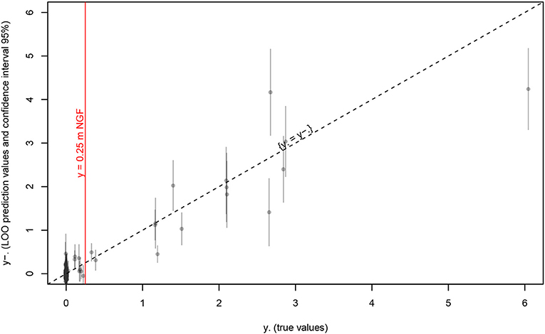
Figure 10. Kriging prediction of max_t(H_p1) vs. true values at the last iteration (19). Gray bars are issued from kriging variance, red line is the safety target, and dashed line is unbiased prediction.

We observe that:

• the target value y ≃ 0.25 is sampled closely by several points (many of them where y ≃ 0);

• these “safety limit” points are quite well-predicted (small bias and confidence interval), but even at this last iteration few points are still underestimated in term of risk (i.e., y_{true value} > y_predicted), but it might be improved with some more iterations;

• although the unsafe zone is not well-predicted (often large confidence interval), this is not a major concern for the result (focusing at max_t(H_p1) < 0.25).

Moreover, along the algorithm iterations the number and accuracy of the interest points increases (i.e., 95% confidence interval and bias decreasing together), so that the safety limit uncertainty decreases at the same time (see Figure 11):

FIGURE 11

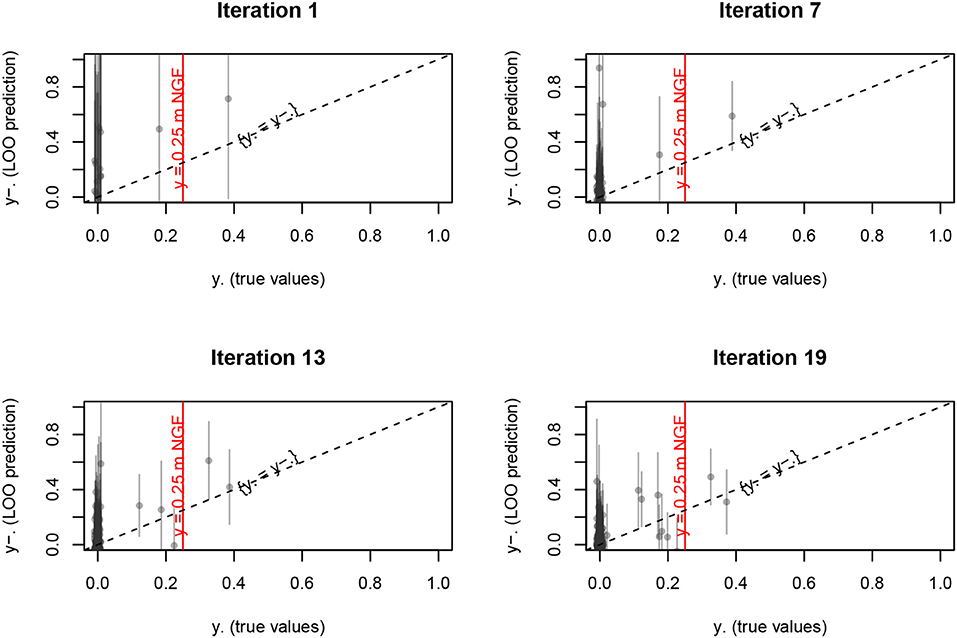
Figure 11. Kriging prediction of max_t(H_p1) vs. the true values at iteration 1, 7, 13, and 19.

5.3. Engineering Analysis

From an engineering perspective, the numerical tool developed in this study (sections 3.1, 3.2, and 3.3) allows us to identify the possible design parameter combinations (Z_a, Z_f) suitable to protect the industrial area against all the possible flooding events identified for the Garonne river (Q_p, T_p) (see all hydrographs simulated in Figure 12):

FIGURE 12

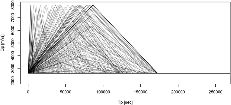
Figure 12. Focused (expected penalizing) flow hydrographs (T_p, Q_p).

In particular, according to the parameters reported in Table 1, we study the combination of the elevation of the industrial basement Z_a and the current dyke height Z_f for all the possible flood events that could cause flooding of the area of interest, and characterized by a peak discharge varying from 2,600 to 8,000 m³/s and a total duration varying from 2 to 48 h. This choice of uncontrolled parameters for the study seems robust considering that the historic flood event for this area does not exceed 6,040 m³/s (SMEPAG, 1989).

The results presented in Figure 6 show that the most relevant parameter for the industrial area's defense against flooding is elevation of the industrial area Z_a. Specifically, the numerical results show that:

• If the basement of the industrial area is elevated above 24 m NGF, the safety criteria is always met even without modification of the current protection.

• On the contrary, if the basement of the industrial area is below 21 m NGF, any modification of the dyke elevation would be useless as the safety criteria is never met.

• An intermediary solution could be to set the basement of the industrial area between 21 and 24 m NGF by controlling the dyke elevation between 22 and 24 m NGF. The optimum point could be chosen according to other practical considerations, like the cost of the civil engineering work (Vrijling, 2001; van Gelder and Vrijling, 2004; Ciullo et al., 2019).

5.4. Perspectives

The general methodology proposed in this study seems quite efficient for designing civil engineering for safety purposes. Although the true penalizing configuration of the worst flood event may have been assumed beforehand (which was at least confirmed by a blind metamodel), it might not be the general case for more complex models (in terms of protection degrees of freedom). It should be noted that the rising number of variables (both controlled and uncontrolled) will have a cost in terms of metamodel predictability, and therefore in terms of the number of simulations needed to achieve enough accuracy for the control set limits. Tuning of such algorithm convergence parameters remains to be done for general cases.

Moreover, the developed numerical tool could be employed in several flooding hazard applications, for instance:

• Quantification of the margins in the existing protections of the civil/industrial area (i.e., the algorithm ensures the protections are robust against any possible flood event).

• Reconstitution of a historical event (i.e., it could be possible to replace the safety criterion with historical knowledge and check for all the possible configurations of the controlled and uncontrolled parameters reproducing the historical data).

Lastly, the primary question that remains is the connection of such an engineering practice to the probabilistic framework often adopted in regulation practice. The mainstream idea should be to weight the hydrograph by their probability of occurrence (thus inside the integral expression of the RSUR criterion), which will link the protection design to the flood return period as required.

In a probabilistic framework, results from this kind of analysis should indicate which return period the protections are associated with and even which return period is hazardous for the civil or industrial installation.

Author Contributions

YR: algorithmic inversion part and computing process. VB: Garonne model and case study definition.

Conflict of Interest

The authors declare that the research was conducted in the absence of any commercial or financial relationships that could be construed as a potential conflict of interest.

Acknowledgments

The authors want to thank Nicole Goutal and Cédric Goeury (EDF R&D) that provide the data necessary for this study.

Footnotes

1. ^Nivellement Général de la France (Above Ordnance Datum).

2. ^Application Program Interface.

3. ^Berkeley Software Distribution.

4. ^This will remain an hypothesis, as long as this black-box algorithm does not consider any physical knowledge about the case study. A deeper physical study might have rigorously excluded any risk for Z_a > 24, for instance.

References

Abily, M., Bertrand, N., Delestre, O., Gourbesville, P., and Duluc, C.-M. (2016). Spatial global sensitivity analysis of high resolution classified topographic data use in 2D urban flood modelling. Environ. Model. Softw. 77, 183–195. doi: 10.1016/j.envsoft.2015.12.002

CrossRef Full Text | Google Scholar

Alho, P., and Mäkinen, J. (2010). Hydraulic parameter estimations of a 2D model validated with sedimentological findings in the point bar environment. Hydrol. Process. 24, 2578–2593. doi: 10.1002/hyp.7671

CrossRef Full Text | Google Scholar

Apel, H., Thieken, A. H., Merz, B., and Blöschl, G. (2004). Flood risk assessment and associated uncertainty. Nat. Haz. Earth Syst. Sci. 4, 295–308. doi: 10.5194/nhess-4-295-2004

CrossRef Full Text | Google Scholar

Bacchi, V., Duluc, C.-M., Bardet, L., Bertrand, N., and Rebour, V. (2018). “Feedback from uncertainties propagation research projects conducted in different hydraulic fields: outcomes for engineering projects and nuclear safety assessment,” in Advances in Hydroinformatics (Springer), 221–241. doi: 10.1007/978-981-10-7218-5_15

CrossRef Full Text | Google Scholar

Bachoc, F. (2013). Cross validation and maximum likelihood estimations of hyper-parameters of Gaussian processes with model misspecification. Comput. Stat. Data Anal. 66, 55–69. doi: 10.1016/j.csda.2013.03.016

CrossRef Full Text | Google Scholar

Bect, J., Ginsbourger, D., Li, L., Picheny, V., and Vazquez, E. (2012). Sequential design of computer experiments for the estimation of a probability of failure. Stat. Comput. 22, 773–793. doi: 10.1007/s11222-011-9241-4

CrossRef Full Text | Google Scholar

Besnard, A., and Goutal, N. (2011). Comparison between 1D and 2D models for hydraulic modeling of a floodplain: case of Garonne River. La Houille Blanche3, 42–47. doi: 10.1051/lhb/2011031

CrossRef Full Text

Bichon, B. J., Eldred, M. S., Swiler, L. P., Mahadevan, S., and McFarland, J. M. (2008). Efficient global reliability analysis for nonlinear implicit performance functions. AIAA J. 46, 2459–2468. doi: 10.2514/1.34321

CrossRef Full Text | Google Scholar

Bozzi, S., Passoni, G., Bernardara, P., Goutal, N., and Arnaud, A. (2015). Roughness and discharge uncertainty in 1D water level calculations. Environ. Model. Assess. 20, 343–353. doi: 10.1007/s10666-014-9430-6

CrossRef Full Text | Google Scholar

Chevalier, C. (2013). Fast Uncertainty Reduction Strategies Relying on Gaussian Process Models (Ph.D. thesis). University of Bern, Bern, Switzerland.

Google Scholar

Chevalier, C., Bect, J., Ginsbourger, D., Vazquez, E., Picheny, V., and Richet, Y. (2014). Fast Parallel kriging-based stepwise uncertainty reduction with application to the identification of an excursion set. Technometrics 56, 455–465. doi: 10.1080/00401706.2013.860918

CrossRef Full Text | Google Scholar

Chevalier, C., and Ginsbourger, D. (2013). “Fast computation of the multi-points expected improvement with applications in batch selection,” in International Conference on Learning and Intelligent Optimization (Berlin; Heidelberg: Springer), 59–69.

Google Scholar

Chevalier, C., Picheny, V. V., and Ginsbourger, D. (2012). KrigInv: Kriging-Based Inversion for Deterministic and Noisy Computer Experiments. Available online at: http://CRAN.R-Project.org/package=KrigInv

Chevalier, C., Richet, Y., and Caplin, G. (2017). RobustInv: Robust Inversion of Expensive Black-Box Functions. French National Institute for Radio-logical Protection; Nuclear Safety (IRSN). Available online at: https://github.com/IRSN/RobustInv.

Ciullo, A., de Bruijn, K. M., Kwakkel, J. H., and Klijn, F. (2019). Accounting for the uncertain effects of hydraulic interactions in optimising embankments heights: proof of principle for the IJssel River. J. Flood Risk Manage. 12:e12532. doi: 10.1111/jfr3.12532

CrossRef Full Text | Google Scholar

Domeneghetti, A., Vorogushyn, S., Castellarin, A., Merz, B., and Brath, A. (2013). Probabilistic flood hazard mapping: effects of uncertain boundary conditions. Hydrol. Earth Syst. Sci. 17, 3127–3140. doi: 10.5194/hess-17-3127-2013

CrossRef Full Text | Google Scholar

Eijgenraam, C., Brekelmans, R., Den Hertog, D., and Roos, K. (2016). Optimal strategies for flood prevention. Manage. Sci. 63, 1644–1656. doi: 10.1287/mnsc.2015.2395

CrossRef Full Text | Google Scholar

Ginsbourger, D., Le Riche, R., and Carraro, L. (2010). “Kriging is well-suited to parallelize optimization. Adaptation learning and optimization,” in Computational Intelligence in Expensive Optimization Problems, eds C. K. Goh and Y. Tenne (Berlin; Heidelberg: Springer), 131–162.

Jones, D. R., Schonlau, M., and Welch, W. J. (1998). Efficient global optimization of expensive black-box functions. J. Glob. Optimiz. 13, 455–492.

Google Scholar

Kind, J. M. (2014). Economically efficient flood protection standards for the Netherlands. J. Flood Risk Manage. 7, 103–117. doi: 10.1111/jfr3.12026

CrossRef Full Text | Google Scholar

Kleijnen, J. P. C. (2015). Design and Analysis of Simulation Experiments, 2nd Edn. Tilburg: Springer.

Google Scholar

Le Riche, R., Girdziušas, R., and Janusevskis, J. (2012). “A study of asynchronous budgeted optimization,” in NIPS Workshop on Bayesian Optimization and Decision Making (Lake Tahoe).

Google Scholar

Löwe, R., Urich, C., Kulahci, M., Radhakrishnan, M., Deletic, A., and Arnbjerg-Nielsen, K. (2018). Simulating flood risk under non-stationary climate and urban development conditions – Experimental setup for multiple hazards and a variety of scenarios. Environ. Model. Softw. 102, 155–171. doi: 10.1016/j.envsoft.2018.01.008

CrossRef Full Text | Google Scholar

LPCB (1983). Vallée de La Garonne - Enquête Sur Les Ruptures de Digues de Décembre 1981 Entre Meilhan et Port Sainte Marie. LPCB.

Google Scholar

Matheron, G. (1973). The intrinsic random functions, and their applications. Adv. Appl. Probab. 5, 439–368.

Google Scholar

Maurizio, M., Luigia, B., Stefano, B., and Roberto, R. (2014). “Effects of river reach discretization on the estimation of the probability of levee failure owing to piping,” in EGU General Assembly Conference Abstracts, Vol. 16. (Vienna).

Google Scholar

Milanesi, L., Pilotti, M., and Ranzi, R. (2015). A conceptual model of people's vulnerability to floods. Water Resour. Res. 51, 182–197. doi: 10.1002/2014WR016172

CrossRef Full Text | Google Scholar

Monod, H., Iooss, B., Mangeant, F., and Prieur, C. (2019). GdR Mascot-Num: Research Group Dealing with Stochastic Methods for the Analysis of Numerical Codes. French National Center for Scientific Research. Available online at: http://www.gdr-mascotnum.fr/

Nguyen, T., Richet, Y., Balayn, P., and Bardet, L. (2015). Propagation des incertitudes dans les modéles hydrauliques 1D. La Houille Blanche 5, 55–62. doi: 10.1051/lhb/20150055

CrossRef Full Text | Google Scholar

Picheny, V., and Ginsbourger, D. (2013). Noisy kriging-based optimization methods: a unified implementation within the Diceoptim Package. Comput. Stat. Data Anal. 71, 1035–1053. doi: 10.1016/j.csda.2013.03.018

CrossRef Full Text | Google Scholar

Polanco, L., and Rice, J. (2014). A reliability-based evaluation of the effects of geometry on levee underseepage potential. Geotech. Geol. Eng. 32, 807–820. doi: 10.1007/s10706-014-9759-2

CrossRef Full Text | Google Scholar

Ranjan, P., Bingham, D., and Michailidis, G. (2008). Sequential experiment design for contour estimation from complex computer codes. Technometrics 50, 527–541. doi: 10.1198/004017008000000541

CrossRef Full Text | Google Scholar

Razavi, S., Tolson, B. A., and Burn, D. H. (2012). Review of surrogate modeling in water resources. Water Resour. Res. 48, 7401. doi: 10.1029/2011WR011527

CrossRef Full Text | Google Scholar

Richet, Y. (2011). Promethee. French National Institute for Radio-logical Protection; Nuclear Safety (IRSN). Available online at: http://promethee.irsn.org

Richet, Y. (2019). Funz. French National Institute for Radio-logical Protection; Nuclear Safety (IRSN). Available online at: http://doc.funz.sh/.

Roustant, O., Ginsbourger, D., and Deville, Y. (2012). “DiceKriging, DiceOptim: two R packages for the analysis of computer experiments by kriging-based metamodeling and optimization. J. Stat. Softw. 51, 1–55. doi: 10.18637/jss.v051.i01

CrossRef Full Text | Google Scholar

Santana-Quintero, L. V., Montano, A. A., and Coello, C. A. C. (2010). “A review of techniques for handling expensive functions in evolutionary multi-objective optimization,” in Computational Intelligence in Expensive Optimization Problems, eds Y. Tenne and C. K. Goh (Berlin; Heidelberg: Springer), 29–59.

Google Scholar

Santner, T. J., Williams, B. J., and Notz, W. I. (2003). The Design and Analysis of Computer Experiments, 1st Edn. New York, NY: Springer-Verlag.

Google Scholar

SMEPAG (1989). Monographie Des Crues de La Garonne (Du Pont Du Roy Au Bec d'Ambès). SMEPAG.

van Dantzig, D. (1956). Economic decision problems for flood prevention. Econometrica 24, 276–287.

Google Scholar

van Gelder, P. H. A. J. M., and Vrijling, J. K. (2004). “Reliability based design of flood defenses and River Dikes,” in Life Time Management of Structures. Available online at: https://www.researchgate.net/profile/Phajm_Gelder/publication/228943806_Reliability_based_design_of_flood_defenses_and_river_dikes/links/004635325941e6b8f7000000.pdf

Google Scholar

Villa-Vialaneix, N., Follador, M., Ratto, M., and Leip, A. (2012). A comparison of eight metamodeling techniques for the simulation of N 2O fluxes and N leaching from corn crops. Environ. Model. Softw. 34, 51–66. doi: 10.1016/j.envsoft.2011.05.003

CrossRef Full Text | Google Scholar

Vrijling, J. K. (2001). Probabilistic design of water defense systems in the Netherlands. Reliabil. Eng. Syst. Safe. 74, 337–344. doi: 10.1016/S0951-8320(01)00082-5

CrossRef Full Text | Google Scholar

White, G. F. (1945). Human Adjustments to Floods. Department of Geography Research, the University of Chicago.

Yazdi, J., and Salehi Neyshabouri, S. A. A. (2014). Adaptive surrogate modeling for optimization of flood control detention dams. Environ. Model. Softw. 61, 106–120. doi: 10.1016/j.envsoft.2014.07.007

CrossRef Full Text | Google Scholar

Annex: Supplementary Information for Implementation

As already mentioned, this study relies on the Funz engine (Richet, 2019) which provides the computing back end to distribute calculations according to the RSUR algorithm. Considering that the reproducibility of this study is a standard deliverable, the following supplementary information details both the software and hardware implementation.

The “master” computer hosting Funz is a basic desktop computer (just running the Funz engine and RSUR algorithm), which will also remotely start the 8 EC2 instances (Script 1), create the SSH tunnels for protocol privacy and install Telemac on each instance.

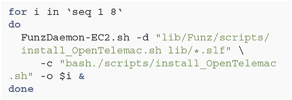
Script 1: Deploy 8 Funz services on EC2, including the Telemac installation.

All TELEMAC-2D calculations are then performed on the 8 servers (suited to the mesh used in this model) started on the Amazon Web Services EC2 cloud computing platform (Screenshot 1).

SCREENSHOT 1

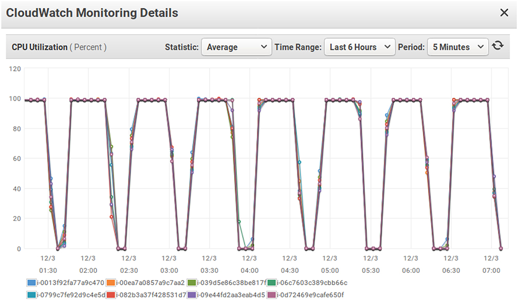
Screenshot 1. 8 Amazon EC2 instances running the Telemac calculations on demand from the RSUR algorithm. Sleep times (non-negligible) are waiting for next RSUR batch.

The main Funz script (Script 2) then starts the RSUR algorithm on the Telemac Garonne model, which is compiled (meaning study parameters are inserted in the template model files) and sent to the EC2 instances as required when the RSUR asks for a calculation point.

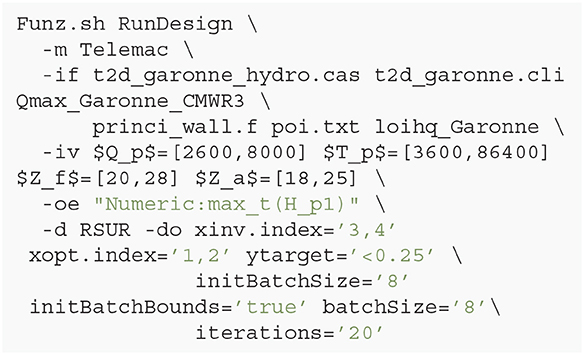
Script 2: The main Funz command which starts the RSUR algorithm on the Telemac Garonne river model (files t2d_garonne_hydro.cas t2d_garonne.cli Qmax_Garonne_CMWR3 princi_wall.f poi.txt loihq_Garonne).

Ultimately, this comprehensive study of 20 RSUR iterations requires about 10 h availability for all computing instances, equating to a cost of less than $100 (at the current standard rates of the main cloud computing platforms).