Synergies or Trade-Offs? Optimizing a Virtual Urban Region to Foster Plant Species Richness, Climate Regulation, and Compactness Under Varying Landscape Composition

Introduction

More than half of the world’s population is now living in cities and the share of urban population is rising further (United Nations Department of Economic and Social Affairs Population Division [UN DESA], 2018). Combined with increasing population globally, urbanization will likely induce an increase in built-up land, with expected impacts on biodiversity (McDonald et al., 2020), the urban climate (Chapman et al., 2017), food security (Abu Hatab et al., 2019) or carbon pools, for instance due to forest loss for land clearing (Seto et al., 2012). Thus, it is imperative to discuss how we want to “grow the world’s cities” (Lin and Fuller, 2013, p. 1161).

In urban planning, one of the main strategies for urban development is a compact city (e.g., Cortinovis et al., 2019) to limit negative effects of urban sprawl, such as increased congestion, greenhouse gas emissions and soil sealing (for many: Yao et al., 2017). However, at least three arguments impede straightforward solutions: First, a variety of ecosystem services (i.e., the benefits humans derive from ecosystems, such as carbon sequestration or water provision, Millennium Ecosystem Assessment, 2005) needs to be considered. In the literature, both direct and indirect relationships between ecosystem services have been documented (Bennett et al., 2009): Direct relationships result from interactions between the services, while indirect relationships are due to the same driver affecting both services. Such a potential common driver is landscape fragmentation. Landscape fragmentation – with intertwined built-up and green areas in a city – is beneficial for local climate regulation, as green spaces providing the cooling and the areas benefiting from that are next to each other. Other ecosystem services might rather benefit from compact green spaces. Such opposite responses indicate trade-offs between ecosystem services, while similar responses indicate synergies (Cord et al., 2017).

The second argument originates from biodiversity conservation. While urbanization threatens many species, urban areas can host more species than intensively used agricultural landscapes, increasing the relevance of cities for biodiversity conservation (Secretariat of the Convention on Biological Diversity, 2012). As a consequence, conserving biodiversity is sometimes a goal of urban planning (Nilon et al., 2017). Species richness (a common measure of biodiversity) in cities, however, heavily depends on the existence of habitats of sufficient size and quality (Beninde et al., 2015). If an increasing compactness of cities is based on the sealing of open, vegetated spaces, it will negatively affect biodiversity (Aronson et al., 2014). It is less clear, though, how habitats should be distributed within cities in order to support high biodiversity. For example, while a number of case studies highlighted negative effects of fragmentation on urban species richness, habitat loss has stronger effects and some organism might even benefit from edge effects imposed by fragmentation (Beninde et al., 2015).

The third argument originates in the land sharing versus land sparing debate applied to cities (Lin and Fuller, 2013). Studies making use of this framework have shown that ecosystem services provision and use can depend on the proportions of different types of land use/land cover in the city (e.g., for pest control: Burkman and Gardiner, 2014; and other ecosystem services: Stott et al., 2015). Also, it matters where these different land uses/land covers are located (e.g., for recreation: Soga et al., 2015). Finally, building density has an indirect influence: It can change the way how the spatial arrangement of the city influences biodiversity (Soga et al., 2014; Villaseñor et al., 2014; Caryl et al., 2016). These studies clearly point out that differentiating building density is crucial for better understanding the impacts of landscape configuration onto biodiversity and ecosystem services in urban landscapes.

Here, we explore whether urban compactness, ecosystem services and biodiversity form a synergistic relationship or whether trade-offs exist. We do so by investigating the spatial configuration of landscapes consisting of blocks with different building densities and varying landscape composition (Table 1). It has to be noted that we do not consider biodiversity as an ecosystem service. While this is sometimes done, the question whether ecosystem services do include biodiversity or not, is under debate (Mace et al., 2012; Silvertown, 2015).

TABLE 1

Table 1. Key terms to describe the landscape used in this study.

One way of exploring the trade-offs or synergies for multiple targets such as species richness and ecosystem services is through the use of spatial optimization of landscapes (Cord et al., 2017). Spatial optimization techniques fall into two types: Pareto-based methods and scalarization. Pareto-based methods generate multiple solutions simultaneously and can consider a (small) number of multiple targets. Methods of scalarization integrate multiple targets into a single target and provide one optimal solution [summary of drawbacks by Duh and Brown (2007)]. Recent reviews of spatial optimization techniques for land use allocation by Yao et al. (2017) and Kaim et al. (2018) provide an overview on such studies and the individual methods available for the two types.

For trade-off analyses with up to four targets, Kaim et al. (2018) suggest Pareto-based algorithms; out of these, genetic algorithms are frequently used. Also, Yao et al. (2017) see a lot of potential for heuristics such as genetic algorithms for optimization studies. So-called “multi-objective genetic algorithms” can find optimal landscapes for the targets that have been specified through quantitative models (Lautenbach et al., 2013; Mouchet et al., 2014). Ideally, optimization of conflicting targets delivers a Pareto-optimal set of landscapes (also called non-dominated solutions). For any given landscape within this set, any improvement in either target would lead to a worsening in at least one other target. Plotting the values of such a set for the case of three targets results in a Pareto frontier as sketched in Figure 1.

FIGURE 1

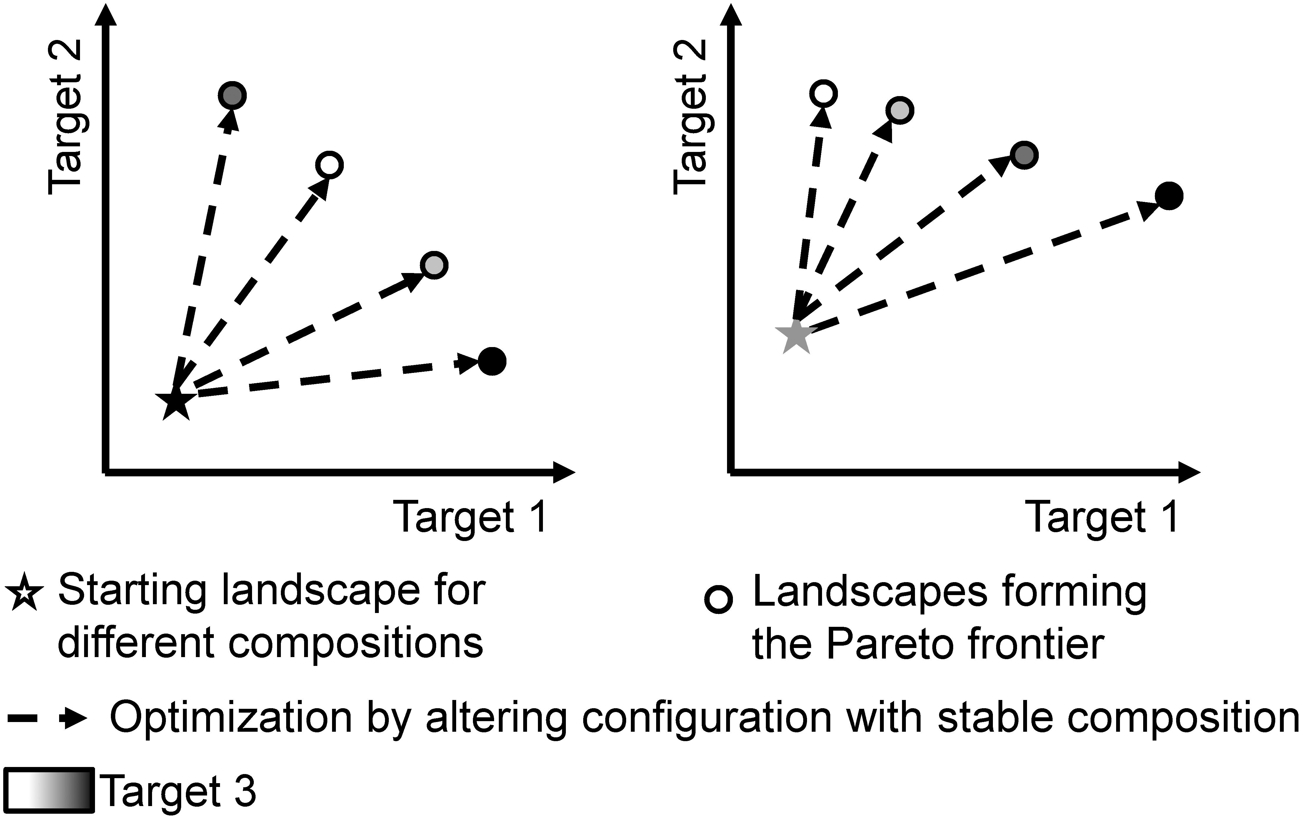
Figure 1. Stylized representation of our optimization approach to explore the effects of landscape composition and configuration. Each scatterplot indicates the levels for three target functions (location and color of the symbols) before (stars) and after (dots) the optimization. The right and left panes of the figure symbolize landscapes with different composition having different values before optimization as well as for their Pareto frontier.

Several studies have used spatial optimization or genetic algorithms for urban land allocation (Table 2), but early work optimized only few spatial entities due to limited computational power. The majority of studies is about optimally allocating additional built-up land into an existing city and, thus, constraints about where and/or which land uses can be converted are implemented. Few studies investigate optimal spatial patterns for building a whole city landscape from scratch. Often, compactness is included as one of the targets for optimization.

TABLE 2

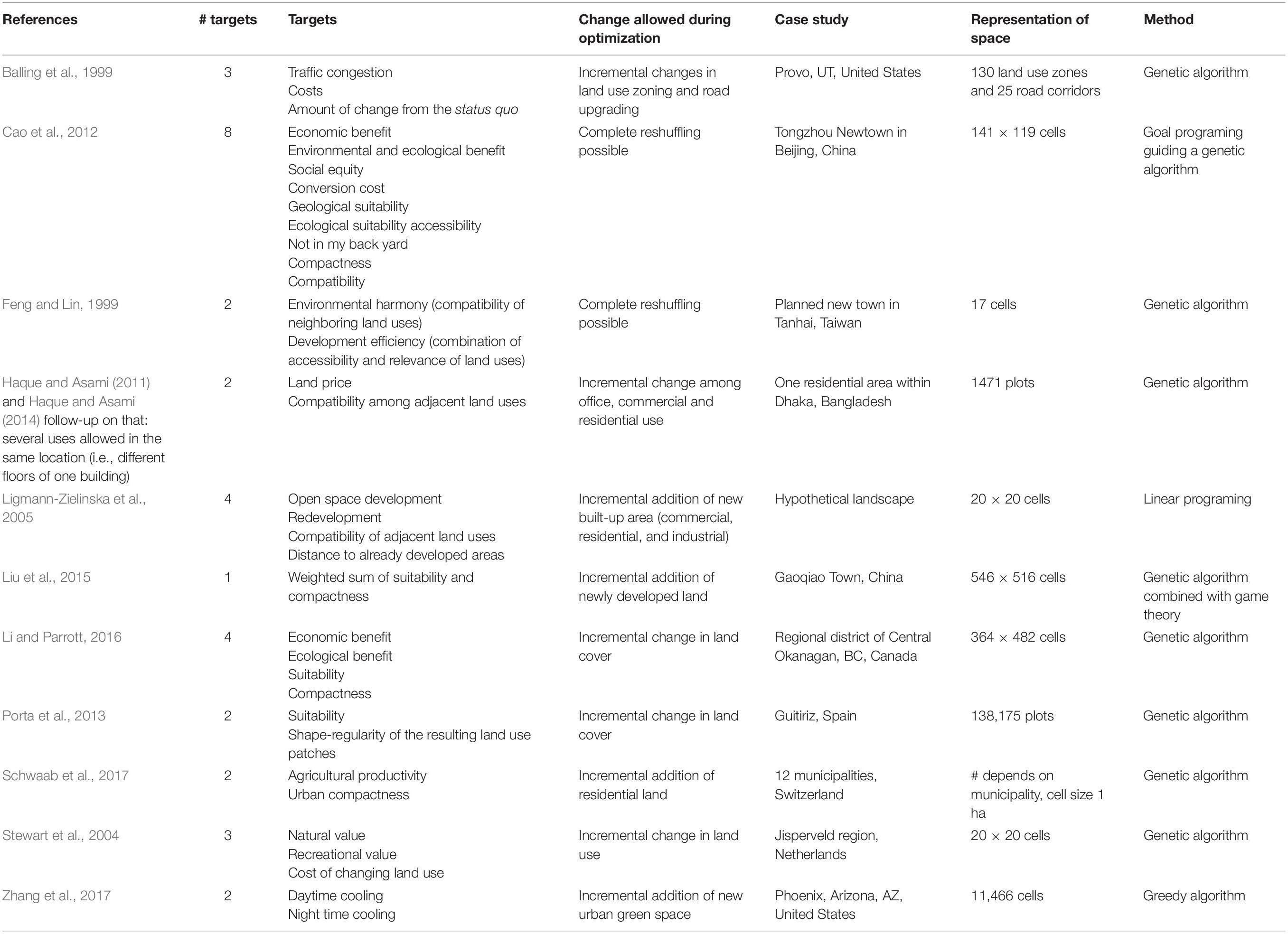
Table 2. Literature review on urban spatial optimization studies.

Our literature review delivered only the studies by Haque and Asami [2011, follow-up in Haque and Asami (2014)] that investigate differences in spatial configuration when landscape composition is changing. In their study of Dhaka, Bangladesh, they vary the changes in residential, commercial and office space. Zhang et al. (2017) included the concept of service providing area and benefiting area. No study compares results for different densities of built-up areas, for instance high- or low-density residential.

In this study, we investigate whether urban compactness, ecosystem services and biodiversity form a synergistic relationship or whether trade-offs exist. We chose local climate regulation since it is an ecosystem service whose production and service areas differ. Biodiversity is quantified as the number of vascular plant species.

We set up a stylized model of an urban landscape consisting of green and built-up cells (Figure 2). At a coarser resolution – the block scale –, we distinguish high- and low-density as well as park blocks. We systematically vary the composition of our city landscape at the block scale, but keep city size constant. This also implies that landscape composition of cell-level land use classes (i.e., green and built-up) remains constant. We optimize this stylized landscape according to our target functions by employing a genetic algorithm. After optimizing the landscapes, we analyze the spatial configurations of the non-dominated solutions per landscape composition at block scale.

FIGURE 2

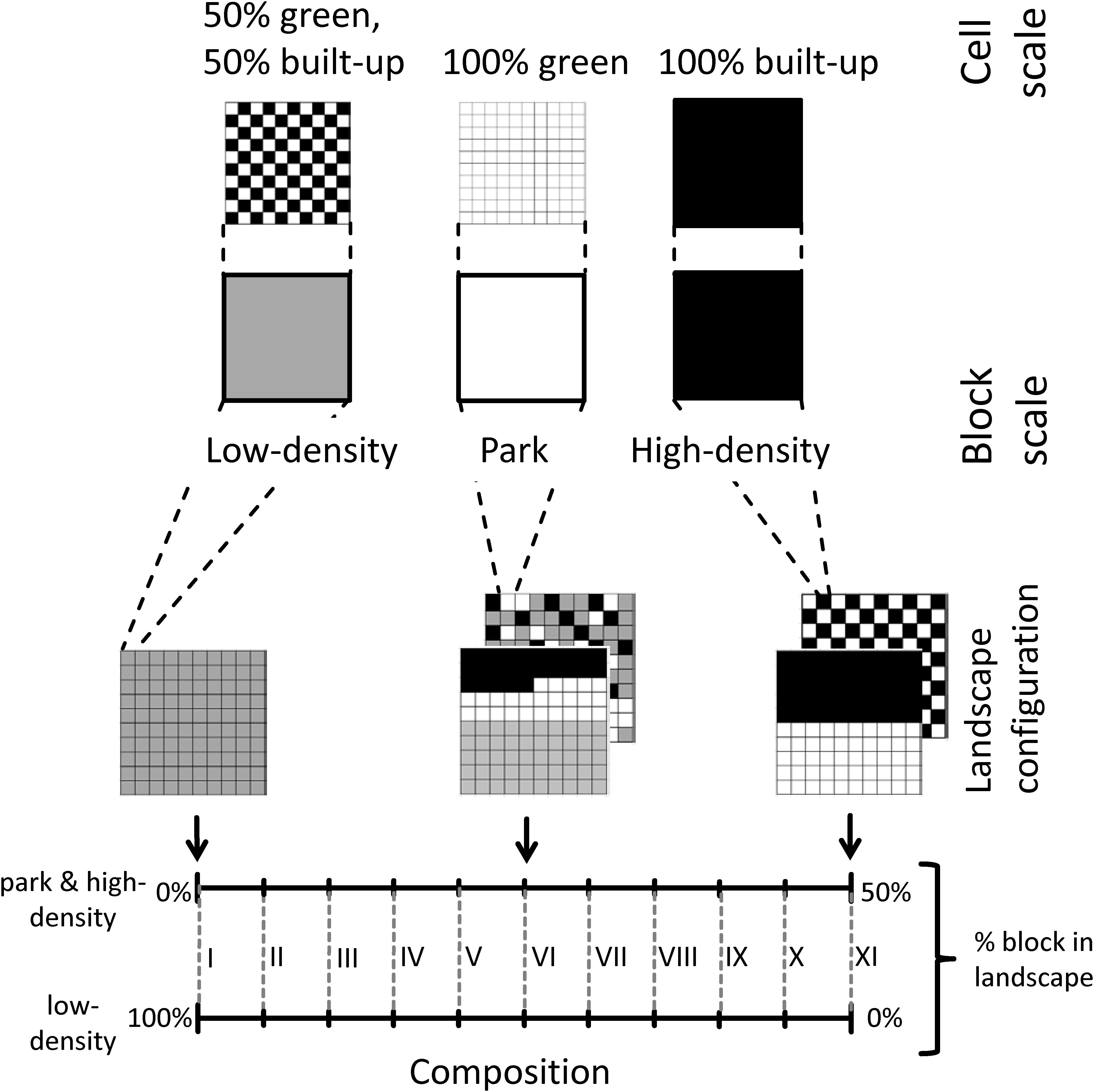
Figure 2. Schematic representation of the virtual city landscape with the translation from cell to block scale (above) and 11 composition settings I to XI and examples of landscape configurations (below).

With our study, we go beyond existing optimization studies for urban landscapes: First, our approach of using a virtual urban region, varying landscape composition at the block scale, allows us to explore the relations among our target functions for different landscape compositions and to check whether optimal landscape configurations remain the same when landscape composition at block scale varies. Using an empirical case study with strong restrictions on feasible changes would not allow such an exploration. Second, we derived two of the target functions from empirical data sets, thus, building on existing empirical ecological relationships. Last, by optimizing urban landscapes from scratch, we hope to find clearer patterns of optimal configurations compared to studies allocating incremental change.

Materials and Methods

Virtual City

We employ a virtual city with a spatial extent of 10 by 10 km² with a total of 10,000 cells of 100 by 100 m² each. We distinguish two spatial scales (Figure 2): cells of 100 × 100 m² size, and blocks consisting of 100 cells (i.e., 1 km² size). In favor of simplicity, cells are either built-up or green. Blocks represent neighborhoods that are

• Park blocks (0% built-up cells, 100% green cells), representing e.g., urban parks or forests,

• Low-density blocks (50% built-up cells, 50% green; arranged in a chessboard pattern), representing e.g., single-family homes with gardens, and

• High-density blocks (100% built-up cells), representing e.g., building blocks without gardens.

When describing the virtual city, we distinguish between landscape composition and landscape configuration. Landscape composition describes which types of land use or land cover are present in a landscape. Here, we operationalized it as the proportion of the park, low- and high-density blocks (Table 1). Landscape configuration describes the spatial arrangement of the land use or land cover classes. In this study, we focus on fragmentation and use Moran’s I as an indicator (Table 1). Furthermore, we include the compactness of built-up blocks as a target function (Table 1, details in section “Quantifying Urban Compactness”).

We fix the size of the city. We do so by keeping the total amount of built-up and green cells equal within any given landscape. Furthermore, we assume the same number of stories for any kind of built-up cell. Thus, two low-density blocks will provide the same number of built-up cells (and floor space) as one high-density block. We vary landscape composition by using different proportions of low-, high-density, and park blocks. As the amount of built-up and green cells are kept equal for both the total city area and the low-density blocks, the proportions of high-density blocks and park blocks are always equal (Figure 2, lower part).

Formalizing the Target Functions

We used empirical relationships of landscape structure and target functions obtained in comparable contexts, i.e., climate zone and overall urban structure. For plant richness and cooling, we made use of empirical data for neighboring cities in the same climate zone (Halle and Leipzig in Central Germany, located ca. 40 km apart from each other). For both target functions, we had access to site-based studies (described in sections “Quantifying Biodiversity” and “Quantifying Local Climate Regulation”) and gradient studies. Urban-rural gradient studies usually describe gradients of vegetation cover, proportion of built-up area or human population density (McDonnell and Hahs, 2008). Often, however, gradient studies use equally sized plots (e.g., Wania et al., 2006; Lososová et al., 2012), not allowing for the calculation of species-area relationships. Also, gradient studies hardly cover spatial interaction effects, for instance effects of neighboring green spaces onto a low- or high-density plot (Schwarz et al., 2012). Therefore, we only used site-based studies and focused on the cell scale, since this was consistent with the spatial resolution of the site-based studies.

Quantifying Biodiversity

Biodiversity can be quantified with a range of indicators, e.g., measures of the richness or abundance of habitats, species, species’ traits or of genetic diversity. We chose the number of species in an area, i.e., species richness for estimating biodiversity. Species richness is easier to measure than functional, genetic or phylogenetic diversity and thus widely applied (Gaston, 2000) and it has been the target of conservation and policy (Ricketts et al., 2005). We focused on the species richness of vascular plants. While former urban studies assessed the effects of land sharing versus land sparing on the diversity of bats (Caryl et al., 2016), birds (Sushinsky et al., 2013) and their predators (Jokimäki et al., 2020), ground beetles and butterflies (Soga et al., 2014), vascular plants have been neglected in the debate. As primary producers, plants are the basis of food webs and they provide many ecosystem services such as carbon sequestration or local climate regulation.

For operationalizing species richness, we re-analyzed data on the number of vascular plant species in 27 protected areas of various size (0.8–120 ha) within the city of Halle (Knapp et al., 2008; Bräuniger et al., 2010; cf. Data Availability Statement). With these data, we fitted a general linear model with quasipoisson-distribution of errors. Quasipoisson distribution is applicable for count data (such as species richness) and does account for overdispersion (Crawley, 2007), which was present in our model. In the model, we predicted the logarithm of number of species with

• Logarithm of the area of the protected site;

• Shape index, calculated as the total edge of the protected area divided by the square root of its area. The shape index indicates the zone of potential interaction with the surroundings, compared to a round shape of equal size;

• The percentage of built-up area in a 500 m buffer around the protected site;

• Nearest neighbor distance, i.e., the distance of one protected area to the next, measured from edge to edge;

and interaction effects between

• Logarithm of the area and shape index;

• Logarithm of the area and percentage of built-up area;

• Logarithm of the area and nearest neighbor distance;

• Shape index and percentage of built-up area.

With the given data, we were not able to distinguish between different types of protected areas such as urban forests, public parks et cetera. This starting model (Table 3, upper row) was simplified during stepwise model reduction, leading to a model with only the logarithm of the area and the shape index as predictors of species richness (Table 3, middle row, Eq. 1). The underlying raw data and the modeled results are depicted in Supplementary Figure S2.1.

TABLE 3

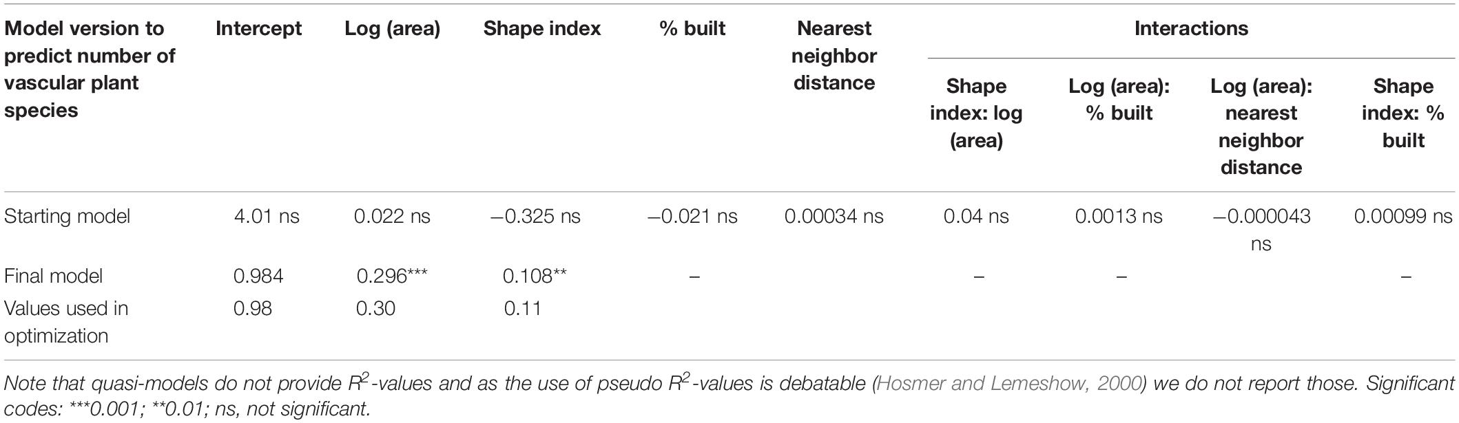
Table 3. Generalized linear model for count data [in R: glm (y ∼ x, family = quasipoisson)], explaining vascular plant species richness.

$$\log \left(species richness\left(i\right)\right)=intercept+slope area\times \log \left(area\left(i\right)\right)+slopeshape\times meanshapeindex(i)(1)$$

with i = green patch.

This simplified model provides an estimation of the logarithm of species richness per patch, with each patch consisting of either one or more adjacent cells of the same density class (sharing an edge, i.e., a von Neumann neighborhood). Thus, each green cell in a low-density block is considered one patch; likewise, a whole park block surrounded by built-up blocks is considered one patch. In order to derive a value to be fitted for the optimization, species richness per patch is normalized by the number of cells for that patch. The arithmetic mean of these normalized patch-level species richness values (i.e., the overall mean per green cell) shall be maximized during optimization. Species richness for built-up patches is set to zero.

Quantifying Local Climate Regulation

Here, we use air temperature measurements to quantify the cooling effects of urban green onto residential areas (e.g., Bowler et al., 2010), as this is directly relevant for urban inhabitants. By doing so, we focus on the flow of this ecosystem service and not solely on its supply. For the optimization, we re-analyzed data sampled by Jaganmohan et al. (2016) for Leipzig, Germany. The authors measured temperature gradients from green spaces into residential surroundings. They quantified cooling effects with (a) maximum temperature difference (delta T max) between a green space and its surroundings and (b) distance at which the cooling effect levels off (cooling distance). In the original empirical study (Jaganmohan et al., 2016), linear regression models were employed to estimate the effects of the following predictors onto maximum temperature difference and cooling distance: size, shape, and type (park versus forest) of urban green spaces and their interactions, percentage of tree/shrub cover within the green space, area of waterbody, distance to city center, type of housing, percentage of tree/shrub cover in 25-m buffer, month of sampling and average wind speed. Adjusted R²-values were 0.42 (cooling distance) and 0.26 (maximum temperature difference).

Since many of these factors were not meaningful in our stylized city (e.g., water bodies, wind speed, or month of sampling), we used the original data to run a simplified linear regression model with only two predictors and their interaction, namely area and shape index (Table 4). The results are used to estimate maximum temperature difference and cooling distance for urban green spaces, i.e., green patches, in the virtual city. In line with the quantification of biodiversity, neighboring cells were combined into patches based on the von Neumann neighborhood, leading to either one cell being one patch (within a low-density block) or at least 100 green cells combined into one park block. Green patches can also consist of more than 100 green cells, if a park block is next to one or more other parks or a low-density block. Thus, the following equations are used to determine the cooling effect of a green patch:

TABLE 4

Table 4. Linear regression model results as basis for the quantification of cooling effects.

$$deltaT\max \left(i\right)=4.7-0.4\times \log \left(area\left(i\right)\right)-3.9\times meanshapeindex\left(i\right)+0.4\times meanshapeindex\left(i\right)\times \log \left(area\left(i\right)\right)(2)$$

with i = green patch.

$$coolingdistance\left(i\right)=-957.3+122.4\times \log \left(area\left(i\right)\right)+363.0\times meanshapeindex\left(i\right)-42.8\times meanshapeindex\left(i\right)\times \log \left(area\left(i\right)\right)(3)$$

with i = green patch.

Results of Eqs 2 and 3 were combined to determine the temperature decrease induced by a specific green patch, assuming a square root function between distance and temperature decrease (Eq. 4).

$$temperaturedecrease\left(x\right)=\frac{deltaT\max \left(i\right)}{\sqrt{coolingdistance\left(i\right)}}\times \sqrt{x}-deltaT\text{\hspace{0.17em}max}(i)(4)$$

with i = green patch and x = distance to green patch i; x < cooling distance.

This simplified model implies, for instance, that a 4 km²-park (four blocks) has a stronger cooling effect at its boundary than smaller parks, and its cooling effect also extends further into the surroundings (Supplementary Figure S2.2). Supplementary Figure S2.2 also indicates the cooling effects of a 1 km²-park surrounded by four high-density blocks and a 1 km²-park surrounded by three high-density blocks, and one low-density block. The latter makes a slightly larger green patch due to the neighboring green cells stemming from the low-density block and has a higher shape index. This leads to cooler temperatures at the boundary, but its cooling effect levels off earlier than for the compact park. In our stylized landscape, a maximal cooling distance of almost 1000 m can be reached if all park blocks are combined in one patch.

The optimization approach requires any target function to deliver a single number at landscape scale. Therefore, the individual temperature effects of individual green patches, first, were mapped onto built-up cells. If a single built-up cell experiences a cooling effect by more than one green patch, the largest cooling effect is considered only, in other words, temperature decreases by several green patches onto the same built-up cell are not added up. After that, the total cooling effect on the landscape scale is quantified as the sum of the cooling effect on built-up cells, divided by the total number of cells. The optimization maximizes the total cooling effect.

Quantifying Urban Compactness

As a third target function, we included urban compactness since a compact city is a goal often pursued in urban planning, for instance to reduce exhaust fumes and soil sealing. Multiple indicators exist to measure urban compactness (Burton, 2002; Tsai, 2005). One of the common indicators to compare compactness across cities is edge density, the total edge of built-up areas divided by the total built-up area (Herold et al., 2002; Schwarz, 2010; Cortinovis et al., 2019). Here, we compare the spatial configuration of the same total built-up area which is divided into low- and high-density blocks, and the proportions of these blocks vary across simulations with different landscape compositions. Thus, we adapt the edge density metric as follows: First, we recode low- and high-density blocks into the same category of built-up blocks, create patches out of them and compute the total edge of these patches. By considering also inner edges (e.g., of a donut-shaped patch), compact patches without holes have smaller values. In order to compare results across different landscape compositions, we normalized the value to range from 0 (maximally dispersed pattern) to 1 (most compact) (Eq. 5). Optimization was then pursued by maximization.

$$compactness=1-\frac{\sum totaledge(j)-minimumedge}{maximumedge-minimumedge}(5)$$

with j = built-up patch; minimum edge = theoretical minimum edge in the landscape given the number of built-up blocks, assuming all built-up blocks are combined in one compact patch; maximum edge = theoretical maximum edge in the landscape for the given number of built-up blocks, assuming all built-up blocks are arranged in a chessboard-style pattern.

Optimizing Landscapes

We employed a multi-objective genetic algorithm (NSGA-II, Deb et al., 2002) to search for optimal spatial configurations regarding the three target functions. Therefore, we used a recently developed landscape optimization tool, CoMOLA (Verhagen et al., 2018; Strauch et al., 2019), that implements inspyred, a free, open source framework for creating biologically inspired computational intelligence algorithms in Python. CoMOLA supports user-defined models or target functions and allows for basic land use constraints, such as limiting the total proportion of each land use class. The software is available at https://github.com/michstrauch/CoMOLA.

Based on an initial landscape and pre-defined constraints, CoMOLA starts an evolutionary process by first creating a set of different yet constraint-satisfying (so-called “feasible”) landscapes. As the algorithm is inspired by biological evolution, its terminology and principles are likewise: Each landscape is called an individual and is represented by a genome, i.e., a string of integers encoding the land use of each grid cell. All landscapes of one generation form a population which changes over generations due to selection and variation (i.e., combination and mutation): Using the target functions described above, each individual is assigned fitness values representing the achieved values for the three targets. The genetic algorithm then applies a Pareto ranking for each individual based on its fitness values. The algorithm archives best individuals and selects individuals for mating to generate a new (offspring) population. In mating, each offspring individual is generated by a random combination (crossover) of two genomes. The likelihood of mating increases for individuals with a higher Pareto rank. Additional random mutations increase the diversity of genomes to consider a wide range of different spatial configurations. Mating can result in constraint-violating (so-called “infeasible”) offspring individuals. Hence, genomes of infeasible individuals are modified using a repair operation specifically developed for land allocation optimization with small tolerance in terms of land use class proportions. The entire procedure, from fitness value calculation to offspring generation and genome repairing, is repeated for a pre-defined number of generations.

Over generations, the Pareto front, i.e., the set of points where no further increase of one target function is possible without decreasing another, successively moves away from the coordinate origin. Considering the vast number of possible landscapes, no optimization algorithm can guarantee to find the global optimum in a finite number of generations; yet, genetic algorithms are known for their good performance in reasonable run-time (Deb et al., 2002). The combination of crossover and mutation prevents them from getting stuck at local optima. To tackle the question of how much run-time/how many generations are needed, we observed the above-mentioned movement of the Pareto front. Technically, we measured the volume (“hypervolume,” Zitzler and Thiele, 1999) the Pareto front spans with the coordinate origin. As its increase slows down, we take that as an indicator for approaching global optima.

To always host the same number of inhabitants in the city and not change city size, we did not allow for changing landscape composition on the cell scale, meaning that always 50% of all cells are green and 50% are built-up. However, on the block scale, landscape composition can vary from 100% low-density blocks to 50% high-density, and 50% park blocks (Figure 1). The optimization algorithm works on the block scale, meaning that the spatial arrangement of blocks is varied, not the cell scale pattern. This allowed us to work with the city size as described in section “Virtual City” with a constrained landscape composition. We ran the optimization for 10 different settings of landscape composition: Low-density blocks in a range from 0 to 90% in intervals of 10%, and high-density and park blocks in a range from 5 to 50% in intervals of 5%, respectively (see also Figure 2). In order to constrain landscape composition in each of the 10 settings, we applied the repair mutation algorithm implemented in CoMOLA (Strauch et al., 2019). For each setting, we ran the optimization for a total of 250 generations with a population size of 50, a crossover rate of 0.9, and a mutation rate of 0.01.

To determine whether two target functions form a trade-off, synergy or do not have a relationship, we investigate pairwise correlations. To account for non-linear relationships (scatterplots in Supplementary Material S1), we use Spearman’s rank correlations.

Results and Discussion

In the following, we present and discuss results of our optimization runs. To ease understanding, we first explore one example simulation (section “Exploring One Example Simulation”), before analyzing whether we find trade-offs or synergies between the target functions (section “Trade-Offs or Synergies in the Virtual City?”) Afterward, we investigate the relations between landscape configuration and the targets (section “Relations With Landscape Configuration”). We close with limitations of our study (section “Limitations of the Study and Future Research”).

Exploring One Example Simulation

Figure 3 depicts the front of non-dominated solutions for plant species richness, cooling and compactness for a park block proportion of 20%, and proportions of 20% high-density, and 60% low-density blocks. The scatterplot indicates a negative relationship, i.e., trade-off, between cooling and plant richness, which is confirmed by a strong negative correlation of r_S = −0.96, p < 0.001 (Table 5). Also, a weaker negative relationship between cooling and compactness is visible (r_S = −0.36, p < 0.001); while the slightly positive relationship between plant richness and compactness is hard to detect (r_S = 0.12, p < 0.05).

FIGURE 3

Figure 3. Front of non-dominated solutions for an example composition of 20% park blocks, 20% high- density, and 60% low-density built-up blocks and maps for solutions with maximum values for cooling (1), compactness (2), and biodiversity (3). The maps indicate the location of parks in white, low-density blocks in gray, and high-density blocks in black.

TABLE 5

Table 5. Correlation matrix for all optimization runs (varying park block proportions) based on Spearman’s rank correlations among the three target functions.

For maximum plant richness, Figure 3 (map 3) shows park blocks organized in four patches, with a Moran’s I value of 0.5 indicating clustering. Parks and low-density blocks (Moran’s I = 0.6) are separated from each other by high-density blocks (Moran’s I = 0.1). This pattern avoids merging individual green cells within the low-density blocks with park blocks. Therefore, the influence of individual green cells on species richness is maximized.

The spatial pattern for maximum compactness (Figure 3, map 2) is easily related back to its target function, which abstracts high- and low-density blocks to built-up. The maximum value is reached for a compact city with a park partly surrounding the built-up center (Moran’s I park = 0.6; Moran’s I for high- and low-density blocks combined = 0.6).

The spatial pattern for maximum cooling (Figure 3, map 1) is different, since here also high-density blocks tend to cluster in one large patch. Thus, all three block types are clustered, which is reflected in similar Moran’s I values of 0.5. When quantifying cooling, low-density blocks are translated to chessboard-like patterns of green and high-density cells at the cell scale. Hence, the green structure at the bottom right is one large green patch with a maximum cooling of 6.6 K at its edge. The large temperature difference is also due to the larger shape index, since the individual green cells of the neighboring low-density blocks are assigned to the large green patch. This is supposedly the reason why the large high-density patch is not adjacent to the large green patch but instead separated by low-density blocks. To further explore this pattern, we compared its cooling effect with a landscape consisting of fully segregated block types, i.e., without any low-density blocks in both the park and the high-density blocks. We found smaller cooling effects onto built-up cells in this landscape, which suggests that the low-density blocks inserted in the park and high-density patches are not accidental results of the mutation but rather stem from the cooling effects of green cells included in the low-density blocks.

Trade-Offs or Synergies in the Virtual City?

When exploring the fronts of non-dominated solutions and the trade-offs/synergies among the three target functions for all optimization runs (Figures 3, 4 and Table 5), the first obvious pattern to notice is the effect of landscape composition at block scale on the target functions, especially plant species richness: A decrease in park blocks, implying at the same time an increasing proportion of low-density blocks, increases plant richness and compactness, but slightly limits the cooling effect. This is reflected in the correlations between the three target functions and proportion of park blocks (Table 5). For compactness, this result is consistent with its definition, i.e., the number of combined patches comprising low- or high-density blocks shall be minimized. The lower the proportion of park blocks in a landscape, the easier it is to achieve high compactness. For cooling, decreasing the proportion of park blocks in the landscape limits its effect since scattered green cells in low-density blocks have a lower capability of extending their cooling effect into the surroundings than park blocks. For plant richness, an increase in richness with a decrease in park block proportion first seems counterintuitive; however, the convex shape of the species-area relationship (Gleason’s exponential curve as a widely used approach for calculating the relationship; Scheiner, 2003) implies that the increase in species richness with an increase in area slows down the larger the area gets. Thus, theoretically, a single green area of e.g., 100 m² surrounded by built-up areas should harbor more species than a green 100 m² area nested within a larger green area (note that neither did the optimization allow accounting for nestedness, nor was the biodiversity data underlying our calculations nested). Chessboard pattern-like low-density blocks will thus be favored, i.e., many single green cells. A range of case studies on the urban-rural gradient showed peaks of species richness at low-density sites [as summarized by Pautasso (2007)], which is in line with our quantification of the target function and the resulting spatial patterns. Green corridors support urban biodiversity across taxa (Beninde et al., 2015), so low-density areas have the potential to support a high number of species as long as they are well connected among each other. Generally, however, there is no standard response of biodiversity to increasing density. Rather, depending on their functional traits, some taxa will decline and some will increase in richness with density, while others will peak in richness at intermediate density (McDonnell and Hahs, 2008). Accordingly, while several studies concluded that urban biodiversity responds less negatively to land sparing than land sharing, they indicate that this response will vary depending on species’ habitat preferences (Soga et al., 2014; Jokimäki et al., 2020) and sensitivity to urbanization (Sushinsky et al., 2013). It needs to be emphasized that we did neither distinguish among groups of plant species (e.g., native versus non-native, rare versus common species or different functional groups) nor did we consider other taxa. Still, the strong relationships of biodiversity and compactness with landscape composition are in line with other studies documenting influences of landscape composition on biodiversity and ecosystem services (Burkman and Gardiner, 2014; Stott et al., 2015).

FIGURE 4

Figure 4. Fronts of non-dominated solutions for cooling, biodiversity, and compactness differentiated by landscape composition with different shares of park blocks (10–50%) in the landscape. Note that the absolute values for biodiversity strongly depend on the share of park blocks in the landscape.

The second, and at a first glance surprising, result is the change of relationships among the three target functions for different landscape compositions at block scale (Figure 4). In fact, the trade-off between plant richness and cooling is the only stable relationship among the three, and highly significant for all park block proportions (Table 5). However, their correlation across all optimization runs is much lower (r_S = −0.19) than for the individual compositions, since the levels of plant richness change considerably with park proportion. Thus, averaging across all optimization runs – and thus different landscape compositions – can provide misleading results. We were only able to discern this by comparing correlations between different, fixed landscape compositions. One likely reason for these changes from synergies to trade-offs due to landscape composition is the different response of the individual target functions to landscape composition which we have discussed above. Since the literature also pointed out moderating effects of landscape composition onto the relationship of configuration and biodiversity, we also investigate these in the next section.

Relations With Landscape Configuration

For plant richness and compactness, we identified a transition from trade-off to synergy with increasing proportions of low-density blocks. Why is this the case? Given our target function, plant richness is highest when green cells are spread over as many patches as possible. For landscapes with a high proportion of parks, built-up blocks mainly consist of high-density blocks. When they form a single built-up block to maximize compactness, parks need to be arranged in a ring around it, thus, creating larger green patches. This is reflected in a strong positive correlation (Table 5) between Moran’s I for parks and compactness for landscapes with a high proportion of park blocks. This, in turn, leads to lower plant richness, and overall to a trade-off between compactness and plant richness for these landscapes. On the contrary, landscapes with a low park proportion achieve maximum values for plant richness when park blocks are separated from low-density blocks so as to avoid forming larger green blocks. One way of achieving this is to surround low-density blocks with high-density blocks, which is visualized in Figure 3. This leads to a synergy between plant richness and compactness for such landscapes.

We also identified such a change for cooling and compactness. For a landscape mainly consisting of parks and high-density blocks, compact, i.e., larger, parks have a positive influence on cooling, likely since their cooling effect at the border is stronger. This is underlined by a positive correlation between Moran’s I for parks and cooling, indicating that more clustered parks are better for cooling in landscapes with many park blocks. This correlation is reversed for low park block proportions (Table 5), meaning that dispersed, small parks have a positive impact on cooling for these landscapes. According to our formulation of the target function (Supplementary Material S2), an increase in shape index leads to a much stronger cooling effect at the boundary of the park for small green patches of almost similar size, while the loss of cooling distance is negligible. Averaging over many different landscape compositions at block scale blurred the effect of a transition between trade-off and synergy.

To complement our analysis, we ran linear regression models to predict the three target functions with the park proportion, Moran’s I for all three block types and one way interactions between park proportion and Moran’s I (Supplementary Material S3). The adjusted R²-values suggest that plant richness and compactness can be completely predicted, while for cooling, at least one predictor is missing.

This finding has a clear implication for the land sharing versus land sparing debate in cities: There is no single answer to the question how to grow the world’s cities, since an optimal spatial configuration of the city depends on its composition. So far, only few other studies have investigated interaction effects between landscape composition and configuration onto biodiversity. For instance, Villaseñor et al. (2014) found interaction effects between landscape composition (housing density) and configuration (urban edge) on forest-dwelling mammals in Australia; and the direction of effects differed per species. Soga et al. (2014) investigated butterflies and ground beetles in Tokyo, Japan, and also found interactions between composition (building density) and configuration, and the responses were different for both taxa. We are not aware of other empirical studies explicitly testing interaction effects between landscape composition and configuration for explaining urban ecosystem services. Also, the two optimization studies that allow for a complete reshuffling of the landscape (Feng and Lin, 1999; Cao et al., 2012) did not investigate changing landscape composition and its effects. The findings of our optimization study thus clearly point out a need for further research.

Limitations of the Study and Future Research

Clearly, we have had to simplify tremendously in order to create the virtual city and quantify our target functions. We took on the challenge of trying to base our target functions on empirical data where possible. Each target function could also be quantified in a different way, for instance by using other indicators for biodiversity than plant species richness; taking into account daytime versus night time cooling (Zhang et al., 2017); or weighting compactness of low- versus high-density blocks differently. Also, since the optimization only varied area and shape of patches in the virtual landscape, many other factors influencing the target functions were not considered, thus limiting the explanatory power of the target functions. Thus, reality is – of course – more complex than the virtual landscape simulated here. What is more, we did not consider how different target functions might interact. For instance, biodiversity can also influence ecosystem services (Schwarz et al., 2017) such as cooling – different habitat types, for example, differ in their cooling potential (Lehmann et al., 2014; Jaganmohan et al., 2016). Further research could investigate to what extent other (also formulations of) target functions imply that trade-offs and synergies depend on landscape composition. Especially functional traits of species have the potential to explain responses of biodiversity to changing landscape composition (Tscharntke et al., 2012) and at the same time they can be linked to ecosystem services, helping us to better understand synergies and trade-offs among services and biodiversity (Schwarz et al., 2017).

Also, we needed to aggregate two of our target functions into one value each for the whole landscape to feed it into the optimization algorithm, since the target functions for plant richness and local climate regulation were quantified at the patch scale, i.e., the number of species per green patch and its cooling effect. Thus, for both indicants, we had to identify ways of integration across the landscape. This is challenging for plant richness, as species-area curves only consider the number of species, not their identity. Summing up the number of species per patch to a total number of species results in double-accounting many species. Our approach of first downscaling species richness of patches onto cells and then maximizing mean species richness per cell (section “Quantifying Biodiversity”) does not prevent that and in fact fosters fragmentation: The species-area relationship is not linear, but logarithmic. Therefore, dividing the estimated species richness per patch by the number of cells leads to high species richness per cell for small patches. For aggregating the cooling effect, it is not clear whether, and if so, to which extent the cooling effects of neighboring green patches onto a specific built-up area are adding up. We decided to use the largest cooling effect onto a single built-up cell stemming from any of the neighboring green patches, but did not add them up as Zhang et al. (2017) did since we had no reliable data on that. Potentially, using process models instead of simple, empirical relationships could circumvent these challenges. However, such process models would pose serious challenges for computation time when used within a genetic algorithm.

For our virtual city, we chose a very simple, stylized landscape. Even within this stylized approach, there is room for further investigation. By introducing an equivalent of high-rise buildings, we may introduce more heterogeneity in terms of block types and thus landscape compositions. This is extremely relevant since urbanization in many parts of the world also means a strong increase in building heights (e.g., Frolking et al., 2013). A challenge related to this is to conceptualize empirical studies that explicitly take into account building height as a covariate. What is more, green infrastructure such as green walls and green roofs (Pauleit et al., 2018) indicate that the differentiation into built-up and green areas is also simplistic, as is the assumption that all green cells are equal, not distinguishing into different habitat types and qualities. Finally, effects of city size need to be explored, as small cities might inhibit patterns that can only evolve in larger cities; also topographic features, average wind directions et cetera would be useful to include.

Finally, we believe more research on modeling stylized cities by building them from scratch (our study, Feng and Lin, 1999; Cao et al., 2012) would be a promising avenue to investigate generic relationships. Also other modeling methods, for instance agent-based modeling, could be worthwhile to explore further, as for instance done by Orsi (2019).

Conclusion

We showed that ecosystem services (here: local climate regulation), biodiversity (here: vascular plant species richness) and one of the main strategies for urban development, i.e., a compact city, do not have a stable relationship but either form synergies or trade-offs, depending on landscape composition. Recent reviews investigating the relationships among biodiversity and a range of ecosystem services showed that these can be positive, neutral, negative, or inexistent (Harrison et al., 2014; Ziter, 2016; Schwarz et al., 2017). While these studies indicated that synergies among different targets of urban planning cannot be taken for granted, we show that landscape composition is a key factor to be considered. Therefore, we strongly suggest researchers to investigate trade-offs and synergies for different landscape compositions, also when using more complex target functions. Such research can result in recommendations to urban policy and planning, especially in countries where rising shares of urban population necessitate re-thinking the allocation of green and built spaces within cities or even the construction of novel cities from scratch. Also, in addition to landscape composition, the size of the landscape/urban region could be varied to see whether basic patterns change.

Urban planning often encounters “wicked problems” (Rittel and Webber, 1973) that, among other issues, do not allow for one single solution that fits all needs. This is also the case here, and even worse, target functions that go hand in hand in one type of landscape are conflicting in others. Our findings also imply that the resolution of the land sharing versus land sparing debate might depend, in large part, on the composition of a given city. This poses an even greater challenge for decision-making in real world situations: For instance, our study suggests that empirical findings on trade-offs and synergies for a specific landscape composition (e.g., city district with specific building density) cannot easily be transferred to another with much higher or lower building density – or another city, for that matter. More research, also including meta-studies (van Vliet et al., 2016), is required to further disentangle the effects of landscape composition onto trade-offs and synergies for urban landscapes.

Data Availability Statement

The datasets generated by the genetic algorithm and analyzed for this study are published on Zenodo (http://doi.org/10.5281/zenodo.3233339). The data on vascular plant species in 27 protected areas within the city of Halle are available under http://www.halle.de/push.aspx?s=downloads/de/Verwaltung/Umwelt/Natur-und-Artenschutz/Schutzgebiete//Landschaftsschutzgebiete/buschendorf_klotz_1996_teil-2_flora_kl.pdf.

Author Contributions

NS, FH, SK, and MS contributed conception and design of the study. NS and SK formalized the target functions. FH and MS simulated optimization runs. FH, MS, and NS performed the statistical analysis. NS wrote the first draft of the manuscript. FH, SK, and MS wrote sections of the manuscript. All authors contributed to manuscript revision, read and approved the submitted version.

Funding

We gratefully thank Helmholtz Centre for Environmental Research – UFZ, Germany, for financial support within the Helmholtz Association’s program-oriented research period III (2014–2020).

Conflict of Interest

The authors declare that the research was conducted in the absence of any commercial or financial relationships that could be construed as a potential conflict of interest.

Acknowledgments

We acknowledge Madhumitha Jaganmohan and Claudia Bräuniger for providing us with the data of their empirical studies. We acknowledge the valuable feedback from the participants of the conference “Modelling Complex Urban Environments” in Waterloo, ON, Canada, June, 2018. Finally, we would like to thank the two reviewers for very constructive comments which helped us to improve the quality of the manuscript.

Supplementary Material

The Supplementary Material for this article can be found online at: https://www.frontiersin.org/articles/10.3389/fenvs.2020.00016/full#supplementary-material

References

Abu Hatab, A., Cavinato, M. E. R., Lindemer, A., and Lagerkvist, C. J. (2019). Urban sprawl, food security and agricultural systems in developing countries: a systematic review of the literature. Cities 94, 129–142. doi: 10.1016/j.cities.2019.06.001

CrossRef Full Text | Google Scholar

Aronson, M. F. J., La Sorte, F. A., Nilon, C. H., Katti, M., Goddard, M. A., Lepczyk, C. A., et al. (2014). A global analysis of the impacts of urbanization on bird and plant diversity reveals key anthropogenic drivers. Proc. R. Soc. B Biol. Sci. 281:20133330. doi: 10.1098/rspb.2013.3330

PubMed Abstract | CrossRef Full Text | Google Scholar

Balling, R., Taber, J. T., Day, K., and Brown, M. R. (1999). Multiobjective urban planning using genetic algorithm. Manager 125, 86–99. doi: 10.1061/(asce)0733-9488(1999)125:2(86)

CrossRef Full Text | Google Scholar

Beninde, J., Veith, M., and Hochkirch, A. (2015). Biodiversity in cities needs space: a meta-analysis of factors determining intra-urban biodiversity variation. Ecol. Lett. 18, 581–592. doi: 10.1111/ele.12427

PubMed Abstract | CrossRef Full Text | Google Scholar

Bennett, E. M., Peterson, G. D., and Gordon, L. J. (2009). Understanding relationships among multiple ecosystem services. Ecol. Lett. 12, 1394–1404. doi: 10.1111/j.1461-0248.2009.01387.x

PubMed Abstract | CrossRef Full Text | Google Scholar

Bowler, D. E., Buyung-Ali, L., Knight, T. M., and Pullin, A. S. (2010). Urban greening to cool towns and cities: a systematic review of the empirical evidence. Landsc. Urban Plan. 97, 147–155. doi: 10.1016/j.landurbplan.2010.05.006

CrossRef Full Text | Google Scholar

Bräuniger, C., Knapp, S., Kühn, I., and Klotz, S. (2010). Testing taxonomic and landscape surrogates for biodiversity in an urban setting. Landsc. Urban Plan. 97, 283–295. doi: 10.1016/j.landurbplan.2010.07.001

CrossRef Full Text | Google Scholar

Burkman, C. E., and Gardiner, M. M. (2014). Urban greenspace composition and landscape context influence natural enemy community composition and function. Biol. Control 75, 58–67. doi: 10.1016/j.biocontrol.2014.02.015

CrossRef Full Text | Google Scholar

Burton, E. (2002). Measuring urban compactness in UK towns and cities. Environ. Plan. BPlann. Des. 29, 219–250. doi: 10.1068/b2713

CrossRef Full Text | Google Scholar

Cao, K., Huang, B., Wang, S., and Lin, H. (2012). Sustainable land use optimization using boundary-based fast genetic algorithm. Comput. Environ. Urban Syst. 36, 257–269. doi: 10.1016/j.compenvurbsys.2011.08.001

CrossRef Full Text | Google Scholar

Caryl, F. M., Lumsden, L. F., van der Ree, R., and Wintle, B. A. (2016). Functional responses of insectivorous bats to increasing housing density support “land-sparing” rather than “land-sharing” urban growth strategies. J. Appl. Ecol. 53, 191–201. doi: 10.1111/1365-2664.12549

CrossRef Full Text | Google Scholar

Chapman, S., Watson, J. E. M., Salazar, A., Thatcher, M., and McAlpine, C. A. (2017). The impact of urbanization and climate change on urban temperatures: a systematic review. Landsc. Ecol. 32, 1921–1935. doi: 10.1007/s10980-017-0561-4

CrossRef Full Text | Google Scholar

Cliff, A. D., and Ord, J. K. (1973). Spatial Autocorrelation. London: Pion.

Google Scholar

Cord, A., Bartkowski, B., Beckmann, M., Dittrich, A., Hermans, K., Kaim, A., et al. (2017). Towards systematic analyses of ecosystem services trade-offs and synergies: current concepts, methods and research gaps. Ecosyst. Serv. 28, 264–272. doi: 10.1016/j.ecoser.2017.07.012

CrossRef Full Text | Google Scholar

Cortinovis, C., Haase, D., Zanon, B., and Geneletti, D. (2019). Is urban spatial development on the right track? Comparing strategies and trends in the European Union. Landsc. Urban Plan. 181, 22–37. doi: 10.1016/j.landurbplan.2018.09.007

PubMed Abstract | CrossRef Full Text | Google Scholar

Crawley, M. (2007). The R Book. Chichester: John Wiley & Sons Ltd.

Google Scholar

Deb, K., Pratap, A., Agarwal, S., and Meyarivan, T. (2002). A fast and elitist multiobjective genetic algorithm: NSGA-II. IEEE Trans. Evol. Comput. 6, 182–197. doi: 10.1109/4235.996017

PubMed Abstract | CrossRef Full Text | Google Scholar

Duh, J., and Brown, D. G. (2007). Knowledge-informed Pareto simulated annealing for multi-objective spatial allocation. Comput. Environ. Urban Syst. 31, 253–281. doi: 10.1016/j.compenvurbsys.2006.08.002

CrossRef Full Text | Google Scholar

Feng, C. M., and Lin, J. J. (1999). Using a genetic algorithm to generate alternative sketch maps for urban planning. Comput. Environ. Urban Syst. 23, 91–108. doi: 10.1016/s0198-9715(99)00004-6

CrossRef Full Text | Google Scholar

Frolking, S., Milliman, T., Seto, K. C., and Friedl, M. A. (2013). A global fingerprint of macro-scale changes in urban structure from 1999 to 2009. Environ. Res. Lett. 8:024004. doi: 10.1088/1748-9326/8/2/024004

CrossRef Full Text | Google Scholar

Gaston, K. J. (2000). Global patterns in biodiversity. Nature 405, 220–227. doi: 10.1038/35012228

PubMed Abstract | CrossRef Full Text | Google Scholar

Haque, A., and Asami, Y. (2011). Optimizing urban land-use allocation: case study of Dhanmondi Residential Area, Dhaka, Bangladesh. Environ. Plan. B Plan. Des. 38, 388–410. doi: 10.1068/b35041

CrossRef Full Text | Google Scholar

Haque, A., and Asami, Y. (2014). Optimizing urban land use allocation for planners and real estate developers. Comput. Environ. Urban Syst. 46, 57–69. doi: 10.1016/j.compenvurbsys.2014.04.004

CrossRef Full Text | Google Scholar

Harrison, P. A., Berry, P. M., Simpson, G., Haslett, J. R., Blicharska, M., Bucur, M., et al. (2014). Linkages between biodiversity attributes and ecosystem services: A systematic review. Ecosyst. Serv. 9, 191–203. doi: 10.1016/j.ecoser.2014.05.006

CrossRef Full Text | Google Scholar

Herold, M., Scepan, J., and Clarke, K. C. (2002). The use of remote sensing and landscape metrics to describe structures and changes in urban land uses. Environ. Plan. A 34, 1443–1458. doi: 10.1068/a3496

CrossRef Full Text | Google Scholar

Hosmer, W. H., and Lemeshow, S. (2000). Applied Logistic Regression, 2nd Edn. Hoboken, NJ: Wiley-Interscience Publication.

Google Scholar

Jaganmohan, M., Knapp, S., Buchmann, C. M., and Schwarz, N. (2016). The bigger, the better? the influence of urban green space design on cooling effects for residential areas. J. Environ. Qual. 45:134. doi: 10.2134/jeq2015.01.0062

PubMed Abstract | CrossRef Full Text | Google Scholar

Jokimäki, J., Suhonen, J., Benedetti, Y., Diaz, M., Kaisanlahti-Jokimäki, M. L., Morelli, F., et al. (2020). Land-sharing vs. land-sparing urban development modulate predator–prey interactions in Europe. Ecol. Appl. e02049. doi: 10.1002/eap.2049

PubMed Abstract | CrossRef Full Text | Google Scholar

Kaim, A., Cord, A. F., and Volk, M. (2018). A review of multi-criteria optimization techniques for agricultural land use allocation. Environ. Model. Softw. 105, 79–93. doi: 10.1016/j.envsoft.2018.03.031

CrossRef Full Text | Google Scholar

Knapp, S., Kühn, I., Mosbrugger, V., and Klotz, S. (2008). Do protected areas in urban and rural landscapes differ in species diversity? Biodivers. Conserv. 17, 1595–1612. doi: 10.1007/s10531-008-9369-5

CrossRef Full Text | Google Scholar

Lautenbach, S., Volk, M., Strauch, M., Whittaker, G., and Seppelt, R. (2013). Optimization-based trade-off analysis of biodiesel crop production for managing an agricultural catchment. Environ. Model. Softw. 48, 98–112. doi: 10.1016/j.envsoft.2013.06.006

CrossRef Full Text | Google Scholar

Lehmann, I., Mathey, J., Rößler, S., Bräuer, A., and Goldberg, V. (2014). Urban vegetation structure types as a methodological approach for identifying ecosystem services - Application to the analysis of micro-climatic effects. Ecol. Ind. 42, 58–72. doi: 10.1016/j.ecolind.2014.02.036

CrossRef Full Text | Google Scholar

Li, X., and Parrott, L. (2016). An improved genetic algorithm for spatial optimization of multi-objective and multi-site land use allocation. Comput., Environ. Urban Syst. 59, 184–194. doi: 10.1016/j.compenvurbsys.2016.07.002

CrossRef Full Text | Google Scholar

Ligmann-Zielinska, A., Church, R., and Jankowski, P. (2005). “Sustainable urban land use allocation with spatial optimization,” in 8th ICA Workshop on Generalisation and Multiple Representation, (Tokyo). Available at: http://www.geocomputation.org/2005/Ligmann.pdf

Google Scholar

Lin, B. B., and Fuller, R. A. (2013). Sharing or sparing? How should we grow the world’s cities? J. Appl. Ecol. 50, 1161–1168. doi: 10.1111/1365-2664.12118

CrossRef Full Text | Google Scholar

Liu, Y., Tang, W., He, J., Liu, Y., Ai, T., and Liu, D. (2015). A land-use spatial optimization model based on genetic optimization and game theory. Comput. Environ. Urban Syst. 49, 1–14. doi: 10.1016/j.compenvurbsys.2014.09.002

CrossRef Full Text | Google Scholar

Lososová, Z., Chytrý, M., Tichý, L., Danihelka, J., Fajmon, K., Hájek, O., et al. (2012). Native and alien floras in urban habitats: a comparison across 32 cities of central Europe. Glob. Ecol. Biogeogr. 21, 545–555. doi: 10.1111/j.1466-8238.2011.00704.x

CrossRef Full Text | Google Scholar

Mace, G. M., Norris, K., and Fitter, A. H. (2012). Biodiversity and ecosystem services: a multilayered relationship. Trends Ecol. Evol. 27, 19–26. doi: 10.1016/j.tree.2011.08.006

PubMed Abstract | CrossRef Full Text | Google Scholar

McDonald, R. I., Mansur, A. V., Ascensão, F., Colbert, M., Crossman, K., Elmqvist, T., et al. (2020). Research gaps in knowledge of the impact of urban growth on biodiversity. Nat. Sustain 3, 16–24. doi: 10.1038/s41893-019-0436-6

CrossRef Full Text | Google Scholar

McDonnell, M. J., and Hahs, A. K. (2008). The use of gradient analysis studies in advancing our understanding of the ecology of urbanizing landscapes: current status and future directions. Landsc. Ecol. 23, 1143–1155. doi: 10.1007/s10980-008-9253-4

CrossRef Full Text | Google Scholar

Millennium Ecosystem Assessment (2005). Ecosystems and Human Well-Being: Synthesis. Washington, DC: Island Press.

Google Scholar

Moran, P. A. P. (1950). Notes on continuous stochastic phenomena. Biometrika 37

Google Scholar

Mouchet, M. A., Lamarque, P., Martín-López, B., Crouzat, E., Gos, P., Byczek, C., et al. (2014). An interdisciplinary methodological guide for quantifying associations between ecosystem services. Glob. Environ. Chang. 28, 298–308. doi: 10.1016/j.gloenvcha.2014.07.012

CrossRef Full Text | Google Scholar

Nilon, C. H., Aronson, M. F., Cilliers, S. S., Dobbs, C., Frazee, L. J., Goddard, M. A., et al. (2017). Planning for the future of urban biodiversity?: a global review of city-scale initiatives. Bioscience 67, 332–342. doi: 10.1093/biosci/bix012

CrossRef Full Text | Google Scholar

Orsi, F. (2019). Centrally located yet close to nature: a prescriptive agent-based model for urban design. Comput., Environ. Urban Syst. 73, 157–170. doi: 10.1016/j.compenvurbsys.2018.10.001

CrossRef Full Text | Google Scholar

Pauleit, S., Ambrose-Oji, B., Andersson, E., Anton, B., Buijs, A., Haase, D., et al. (2018). Advancing urban green infrastructure in Europe: outcomes and reflections from the GREEN SURGE project. Urban For. Urban Green. 40, 4–16. doi: 10.1016/j.ufug.2018.10.006

CrossRef Full Text | Google Scholar

Pautasso, M. (2007). Scale dependence of the correlation between human population presence and vertebrate and plant species richness. Ecol. Lett. 10, 16–24. doi: 10.1111/j.1461-0248.2006.00993.x

PubMed Abstract | CrossRef Full Text | Google Scholar

Porta, J., Parapar, J., Doallo, R., Rivera, F. F., Santé, I., and Crecente, R. (2013). High performance genetic algorithm for land use planning. Comput. Environ. Urban Syst. 37, 45–58. doi: 10.1016/j.compenvurbsys.2012.05.003

CrossRef Full Text | Google Scholar

Ricketts, T. H., Dinerstein, E., Boucher, T., Brooks, T. M., Butchart, S. H. M., Hoffmann, M., et al. (2005). Pinpointing and preventing imminent extinctions. Proc. Natl. Acad. Sci. U.S.A. 102, 18497–18501. doi: 10.1073/pnas.0509060102

PubMed Abstract | CrossRef Full Text | Google Scholar

Rittel, H. W. J., and Webber, M. M. (1973). Dilemmas in a general theory of planning. Policy Sci. 4, 155–169. doi: 10.1007/bf01405730

CrossRef Full Text | Google Scholar

Scheiner, S. M. (2003). Six types of species-area curves. Glob. Ecol. Biogeogr. 12, 441–447. doi: 10.1046/j.1466-822X.2003.00061.x

CrossRef Full Text | Google Scholar

Schwaab, J., Deb, K., Goodman, E., Lautenbach, S., van Strien, M., and Grêt-Regamey, A. (2017). Reducing the loss of agricultural productivity due to compact urban development in municipalities of Switzerland. Comput. Environ. Urban Syst. 65, 162–177. doi: 10.1016/j.compenvurbsys.2017.06.005

CrossRef Full Text | Google Scholar

Schwarz, N. (2010). Urban form revisited-Selecting indicators for characterising European cities. Landsc. Urban Plan. 96, 29–47. doi: 10.1016/j.landurbplan.2010.01.007

CrossRef Full Text | Google Scholar

Schwarz, N., Moretti, M., Bugalho, M. N., Davies, Z. G., Haase, D., Hack, J., et al. (2017). Understanding biodiversity-ecosystem service relationships in urban areas: A comprehensive literature review. Ecosyst. Serv. 27, 161–171. doi: 10.1016/j.ecoser.2017.08.014

CrossRef Full Text | Google Scholar

Schwarz, N., Schlink, U., Franck, U., and Großmann, K. (2012). Relationship of land surface and air temperatures and its implications for quantifying urban heat island indicators - An application for the city of Leipzig (Germany). Ecol. Indic. 18, 693–704. doi: 10.1016/j.ecolind.2012.01.001

CrossRef Full Text | Google Scholar

Secretariat of the Convention on Biological Diversity (2012). Cities and Biodiversity Outlook. Stockholm: Stockholm University.

Google Scholar

Seto, K. C., Güneralp, B., and Hutyra, L. R. (2012). Global forecasts of urban expansion to 2030 and direct impacts on biodiversity and carbon pools. Proc. Natl. Acad. Sci. U.S.A. 109, 16083–16088. doi: 10.1073/pnas.1211658109

PubMed Abstract | CrossRef Full Text | Google Scholar

Silvertown, J. (2015). Have ecosystem services been oversold? Trends Ecol. Evol 30, 641–648. doi: 10.1016/j.tree.2015.08.007

PubMed Abstract | CrossRef Full Text | Google Scholar

Soga, M., Yamaura, Y., Aikoh, T., Shoji, Y., Kubo, T., and Gaston, K. J. (2015). Reducing the extinction of experience: association between urban form and recreational use of public greenspace. Landsc. Urban Plan. 143, 69–75. doi: 10.1016/j.landurbplan.2015.06.003

CrossRef Full Text | Google Scholar

Soga, M., Yamaura, Y., Koike, S., and Gaston, K. J. (2014). Land sharing vs. land sparing: does the compact city reconcile urban development and biodiversity conservation?. J. Appl. Ecol. 51, 1378–1386. doi: 10.1111/1365-2664.12280

CrossRef Full Text | Google Scholar

Stewart, T. J., Janssen, R., and Van Herwijnen, M. (2004). A genetic algorithm approach to multiobjective land use planning. Comput. Oper. Res. 31, 2293–2313. doi: 10.1016/s0305-0548(03)00188-6

CrossRef Full Text | Google Scholar

Stott, I., Soga, M., Inger, R., and Gaston, K. J. (2015). Land sparing is crucial for urban ecosystem services. Front. Ecol. Environ. 13:387–393. doi: 10.1890/140286

CrossRef Full Text | Google Scholar

Strauch, M., Cord, A., Pätzold, C., Sven, L., Kaim, A., Christian, S., et al. (2019). Constraints in multi-objective optimization of land use allocation – repair or penalize? Environ. Model. Softw. 118, 241–251. doi: 10.1016/j.envsoft.2019.05.003

CrossRef Full Text | Google Scholar

Sushinsky, J. R., Rhodes, J. R., Possingham, H. P., Gill, T. K., and Fuller, R. A. (2013). How should we grow cities to minimize their biodiversity impacts? Glob. Chang. Biol. 19, 401–410. doi: 10.1111/gcb.12055

PubMed Abstract | CrossRef Full Text | Google Scholar

Tsai, Y. H. (2005). Quantifying urban form: compactness versus “sprawl.”. Urban Stud. 42, 141–161. doi: 10.1080/0042098042000309748

CrossRef Full Text | Google Scholar

Tscharntke, T., Tylianakis, J. M., Rand, T. A., Didham, R. K., Fahrig, L., Batáry, P., et al. (2012). Landscape moderation of biodiversity patterns and processes - eight hypotheses. Biol. Rev. 87, 661–685. doi: 10.1111/j.1469-185X.2011.00216.x

PubMed Abstract | CrossRef Full Text | Google Scholar

United Nations Department of Economic and Social Affairs Population Division [UN DESA] (2018). World Urbanization Prospects: The 2018 Revision. New York, NY: UN DESA.

Google Scholar

van Vliet, J., Magliocca, N. R., Büchner, B., Cook, E., Rey Benayas, J. M., Ellis, E. C., et al. (2016). Meta-studies in land use science: current coverage and prospects. Ambio 45, 15–28. doi: 10.1007/s13280-015-0699-8

PubMed Abstract | CrossRef Full Text | Google Scholar

Verhagen, W., Zanden, E. H., Van Der, Strauch, M., Teeffelen, A. J. A., and Van, et al. (2018). Optimizing the allocation of agri-environment measures to navigate the trade-offs between ecosystem services, biodiversity and agricultural production. Environ. Sci. Policy 84, 186–196. doi: 10.1016/j.envsci.2018.03.013

CrossRef Full Text | Google Scholar

Villaseñor, N. R., Driscoll, D. A., Escobar, M. A. H., Gibbons, P., and Lindenmayer, D. B. (2014). Urbanization impacts on mammals across urban-forest edges and a predictive model of edge effects. PLoS One 9:7036. doi: 10.1371/journal.pone.0097036

PubMed Abstract | CrossRef Full Text | Google Scholar

Wania, A., Kühn, I., and Klotz, S. (2006). Plant richness patterns in agricultural and urban landscapes in central Germany - Spatial gradients of species richness. Landsc. Urban Plan. 75, 97–110. doi: 10.1016/j.landurbplan.2004.12.006

CrossRef Full Text | Google Scholar

Yao, J., Zhang, X., and Murray, A. T. (2017). Spatial optimization for land-use allocation. Int. Reg. Sci. Rev. 41:016001761772855. doi: 10.1177/0160017617728551

CrossRef Full Text | Google Scholar

Zhang, Y., Murray, A. T., and Turner, B. L. (2017). Optimizing green space locations to reduce daytime and nighttime urban heat island effects in Phoenix. Arizona. Landsc. Urban Plan. 165, 162–171. doi: 10.1016/j.landurbplan.2017.04.009

CrossRef Full Text | Google Scholar

Ziter, C. (2016). The biodiversity–ecosystem service relationship in urban areas: a quantitative review. Oikos 125, 761–768. doi: 10.1111/oik.02883

CrossRef Full Text | Google Scholar

Zitzler, E., and Thiele, L. (1999). Multiobjective evolutionary algorithms: a comparative case study and the strength Pareto approach. IEEE Trans. Evol. Comput. 3, 257–271. doi: 10.1109/4235.797969

CrossRef Full Text | Google Scholar