On the Role of Biogeochemical Coupling Between Sympagic and Pelagic Ecosystem Compartments for Primary and Secondary Production in the Barents Sea

Introduction

The Arctic Ocean is one of the environments experiencing the most severe changes due to ongoing climate change (Anisimov and Fitzharris, 2001; Bennett et al., 2015), exemplified by the extent of summer sea ice retreat (Stroeve and Notz, 2018). The current rate of decrease in summer ice cover is estimated to be 13.5% (Peng and Meier, 2018) per decade, with commensurate changes in ice thickness (Lindsay and Schweiger, 2015). Forecasts predict an Arctic Ocean completely free of ice within 30 years (Wang and Overland, 2012) and possibly by 2030 (Diebold and Rudebusch, 2019). These factors all contribute to an earlier exposure of the ocean surface to the atmosphere in spring and ice-free conditions over a longer season (Stroeve et al., 2012; Meier, 2017). All of these changes impact on the physical and ecological characteristic of the Arctic Ocean (Darnis et al., 2012), and its role in the air-sea interface interaction (Cottier et al., 2017; McPhee, 2017).

Sea ice is an essential component of Arctic ecosystems, acting both as a physical barrier to light, wind and dispersion (Clark et al., 2017; Bouchard et al., 2018), and as a substrate for living organisms. The presence of ice modifies and influences exchanges between the atmosphere and the water column such as nutrient deposition, wind stress, water mixing, and light availability, which in turn affects primary production. Moreover, sea ice represents a habitat for a rich microorganism community, mainly composed of microalgae (Thomas, 2017). Ice algae communities play an important role in Arctic ecosystems by contributing to primary production. Sympagic production contributes 3–25%, and in some regions such as the central Arctic, more than 50% of the total primary production (Legendre et al., 1992; Gosselin et al., 1997; Kohlbach et al., 2016). Ice algae also represent a valuable resource for zooplankton grazers, such as copepods (Runge and Ingram, 1991; Leu et al., 2011), amphipods (Werner, 1997), or krill (Stretch et al., 1988; Kohlbach et al., 2017a). In the Arctic shelves, ice algae can also be a key resource early in the season for benthic organisms when they settle to the seabed after ice melt (Søreide et al., 2013; Schollmeier et al., 2018). Ice algae are important for the phenology of pelagic and benthic organisms which rely on this additional energy source for reproduction and growth in spring (McMahon et al., 2006; Søreide et al., 2010), and have a key role in the benthic communities’ structure and dynamic (Kohlbach et al., 2019).

An especially productive Arctic region is the Barents Sea (Sakshaug et al., 2009). In the Barents Sea, sea-ice algae can locally represent around 20% of the total primary production (Hegseth, 1998). However, winter sea ice extent in the Barents Sea has substantially decreased especially since around 1990 (Årthun et al., 2012). Impacts of the sea ice decrease on the primary and secondary production phenology and amplitude remain poorly understood in the Arctic and in the Barents Sea. Some studies already highlight a potential mismatch between ice algae production and zooplankton production and suggest important consequences for the reproduction of copepods (Leu et al., 2011; Dezutter et al., 2019). For example, the reproduction of Calanus glacialis has been found to coincide with the spring ice algae bloom while hatching of eggs coincides with the phytoplankton bloom (Søreide et al., 2010). In the Barents Sea around 80% of zooplanktonic biomass consists of copepod species, of which most, such as C. glacialis and Calanus finmarchicus, can actively feed on sea-ice algae attached to the ice (Runge and Ingram, 1988, 1991), as well as on ice algae released to the water column during the melting process (Michel et al., 1996). While living ice algae cells are important for the zooplankton, dead cells are of relevance for benthic organisms. Few ice algae can survive in the water column and most of them are rapidly exported to the sea floor after ice melt where they contribute to benthic production (Ambrose et al., 2005; Juul-Pedersen et al., 2008; Boetius et al., 2013). Rich in polyunsaturated fatty acids, ice algae represent a valuable food for benthos and play a key role in the detritivorous feed web (McMahon et al., 2006; Sun et al., 2007). For example, Søreide et al. (2013) showed that benthos principally uses particulate organic matter originating from ice algae in the Svalbard region and highlighted that changes in the ice algae production can affect the pelagic and benthic systems. In this context it is essential to thoroughly understand sea-ice algae phenology and its linkage with the pelagic and benthic ecosystems when aiming to identify future changes in the Arctic ecosystem.

Because the Arctic is an extreme environment, in situ observations are not readily available and are often limited to the spring-summer season. Under these circumstances numerical models become a tool of choice for studies covering large spatial and temporal scales. In the last 20 years, there have been important improvements in the modeling of sea ice biogeochemistry (Steiner et al., 2016; Vancoppenolle and Tedesco, 2017). First models were developed and parametrized in a 1D framework focusing on specific locations (Arrigo et al., 1993; Lavoie et al., 2005) and particular processes, for example, the complex brine dynamic and nutrient exchange across the ice-ocean interface (Vancoppenolle et al., 2010). These 1D studies were supported by improvements in understanding of the biogeochemistry and dynamic of the Arctic ecosystem (Yakubov et al., 2019). The studies highlighted instances where ice algae could seed pelagic phytoplankton growth and modify the timing of pelagic primary production (Jin et al., 2006, 2007; Tedesco and Vichi, 2010), and how ice algae could control pelagic phytoplankton biomass by competing for nutrients in the surface water (Mortenson et al., 2017). Subsequently, sea ice modeling has been extended to a 3D framework simulating large-scale primary production in the whole Arctic basin (Deal et al., 2011) or more regional area such as the Hudson Bay System (Sibert et al., 2010). In spite of these recent improvements in the biogeochemical modeling, the linkages between the sympagic, pelagic and benthic systems are still poorly represented.

In order to improve knowledge and understanding of the linkage between the sympagic, pelagic and benthic ecosystems, we present here an enhanced version of the biogeochemical model ECOSMO II (Daewel and Schrum, 2013) implemented for the Barents Sea, to include a fully coupled sympagic system. With recent developments of the ECOSMO-E2E (Daewel et al., 2019), the model will then later allow us to explore ecosystem dynamic including predators such as fishes and macrobenthos. These two components (fish and macrobenthos) are dependent on high-quality sea-ice algae food source (Sun et al., 2009; Søreide et al., 2013) and should be linked to the sympagic system to accurately represent Arctic ecosystem dynamic. We used the model in a 1D application to comparatively assess three characteristic regions of the Barents Sea and investigated (1) the importance of linkages between the pelagic and the sympagic systems for ecosystem dynamics; (2) the relative contribution of the ice algae on the total primary and secondary production; and (3) how variability in ice coverage affects Arctic food-web dynamics.

Materials and Methods

We present here a new version of the ECOSMO II (Daewel et al., 2019) model including a new sympagic (sea-ice biogeochemistry) module and its application to the Barents Sea region. The biogeochemical model was built with the Fortran-based Framework for Aquatic Biogeochemical Models (FABM) (Bruggeman and Bolding, 2014) in order to facilitate coupling to the physical model described below (section Physical model and forcing data). Here we work in a 1D numerical framework, which allows model parameterization, verification, sensitivity tests to study process level with a low computation effort without add complex hydrodynamic processes. Therefore, this approach neglects horizontal transport and only take into account vertical exchange processes.

Model Description

Physical Model and Forcing Data

Physical processes in the water column are calculated by the 1D General Ocean Turbulence Model (GOTM) (Burchard et al., 1999). The simulation resolves the profiles of velocities, temperature, salinity, turbulent mixing, and transport of ecosystem state variables in 50 vertical layers. The physical environment affects the ecosystem dynamics, while an ecosystem feedback to the physics, e.g., heating or albedo is switched off. Photosynthetically available radiation is calculated based on the ecosystem tracers in water and ice as described below. At the surface, the model is forced with atmospheric conditions from the NCEP-R2 reanalysis [NCEP-DOE AMIP-II Reanalysis (R-2); Kanamitsu et al., 2002], and sea ice thickness, sea ice concentration and snow thickness are prescribed from a hindcast simulation with the HYCOM (HYbrid Coordinate Ocean Model) (Bleck, 2002) using a setup based on a model version described in Samuelsen et al. (2015). Tidal currents are prescribed M2 and S2 components of the horizontal velocity in order to parameterize tidal mixing and a spring-neap cycle. Tidal variability of the sea surface elevation is neglected for the present study. Physical conditions are initialized from the World Ocean Atlas v2013 (Boyer et al., 2013), which is also used for a filtered restoring of salinities to the climatological conditions in order to parameterize horizontal fluxes of fresh water. The ecosystem model dynamics are coupled with the FABM framework (Bruggeman and Bolding, 2014) into the 1D model, integrated with a third-order Runge–Kutta ODE solver (Schober et al., 2014), and transported in the vertical due to sinking, vertical advection, and turbulent mixing. The 1D model framework provides a consistent scheme for the analysis of ice-ocean ecosystem exchange fluxes, while horizontal triggers are included only through nudging of salinities and forcing with ice conditions.

Biogeochemical Sea Ice Processes

The ECOSMO II model (Schrum et al., 2006; Daewel and Schrum, 2013), including pelagic and benthic biological and geochemical components, has been adapted here for the Arctic ecosystem. One of the most important characteristics of the Arctic ecosystem is the presence of a sea ice cover and the associated microbial communities, forming a sympagic system (Thomas, 2017). To make the existing ecosystem model applicable to the Arctic, a sympagic system model is required that allows online coupling to the existing model for the pelagic and benthic systems. To achieve this, we added six state variables to the original ECOSMO II model framework, accounting for: one sea-ice algae functional group (IA), four nutrients variables (phosphate PO₄, nitrate NO₃, ammonium NH₄, and silicate SiO₂), and one detritus variable (ID) (Figure 1).

FIGURE 1

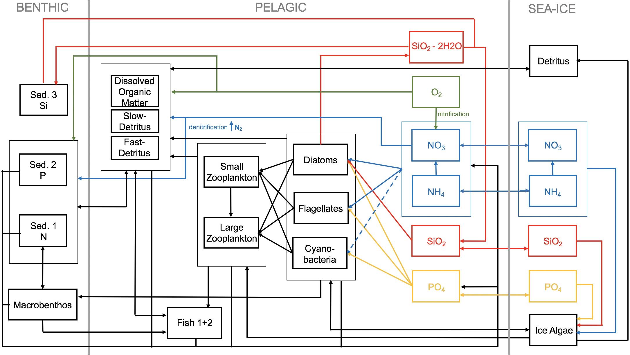
Figure 1. Schematic diagram of the coupled sea-ice ocean model ECOSMO-E2E. The three system (benthic, pelagic, and sympagic) are included. Sed. 1, nitrate/carbon sediment pool; Sed. 2, phosphate sediment pool; Sed. 3, silicate sediment pool.

Arctic sea ice supports a highly diverse microbial community (Arrigo, 2014; Thomas, 2017). Many species of algae bloom in succession throughout the annual season (Hegseth, 1992; Ambrose et al., 2005). Several studies have emphasized the dominance of diatoms (Werner et al., 2007), especially Nitzschia frigida and Melosira arctica (Horner and Alexander, 1972; Gosselin et al., 1997). However, the ECOSMO II model represents functional groups instead of species, and the entire ice algae community approach is represented by a single state variable. Following the assumption that diatoms are dominant in the system, the group processes are parametrized for diatom species.

Similar to the pelagic environment, ice algae dynamics are influenced by various abiotic and biotic factors such as temperature, salinity, light, nutrients, and consumption by microorganisms (Arrigo et al., 1993; Werner, 1997; Arrigo, 2014; Galindo et al., 2017; Oziel et al., 2019). The rate of change in the ice algae biomass is calculated as follows:

$$\frac{\partial IA}{\partial t}=\mathrm{\sigma }\left[IA\right]-\text{M}\left[IA\right]-G\left[IA\right]+G_{\mathrm{ice}\mathrm{\_}\mathrm{flux}}[IA](1)$$

where IA is the sea-ice algae biomass in mgC m^–2. The first term in Eq. 1 represents the gross primary production of ice algae, the second and third term account for the loss of ice algae and the fourth term parametrizes the exchange between ice and water column. The ice algae growth σ depends on the ambient temperature and salinity of brine in the cracks and channels in the ice and can be limited by light and nutrient. We assume a single limiting factor approach rather than multiplicative limitation, such that the specific growth rate is given by:

$$\mathrm{\sigma }\left[IA\right]=\left({\mathrm{\sigma }}_{\text{max}}\times f_T\times f_S\times \text{min}(N_{\text{lim}},L_{\text{lim}})\right)\times \left[IA\right](2)$$

Where σ_max is the maximum growth rate (Table 1). f_T and f_S are respectively, the temperature and salinity dependence of the sea-ice algae growth, and N_lim and L_lim account for nutrient and light limitation respectively. Laboratory experiments have shown that algal growth is influenced by these two factors especially when salinities reach high values in the brine (Arrigo and Sullivan, 1992). According to Vancoppenolle and Tedesco (2017) temperature and salinity dependencies are expressed as following:

$$f_T=e^{r_g\times T}(3)$$

$$f_S=e^{-{\left(2.16-{8.310}^{-5}\times S^{2.11}-0.55\times \ln \left(S\right)\right)}^2}(4)$$

TABLE 1

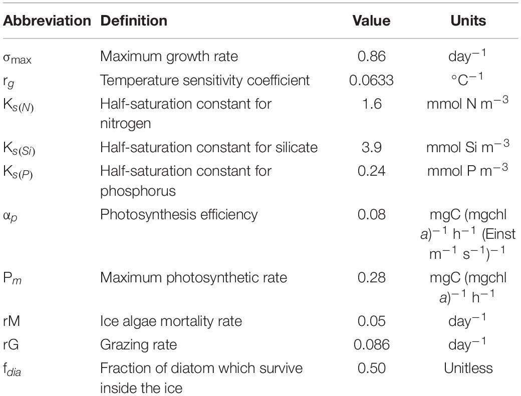
Table 1. List of parameters, corresponding description, and units used in the model for ice algae dynamic.

The terms T and S are, respectively, the ambient temperature in °C and salinity, r_g is the temperature sensitivity coefficient (Table 1). The availability of light and nutrients are the two main factors limiting the ice algae growth with different seasonal relevance (during the polar night in winter for light, and during the summer season for nutrients). The ice algae growth is therefore limited by the four nutrients (NO₃, NH₄, PO₄, and SiO₂) following a Monod-formulation (Monod, 1949). Even though nutrient stoichiometry inside the ice algae is known to be variable, we assume a fixed Redfield stoichiometry (Vancoppenolle and Tedesco, 2017; Selz et al., 2018).

$$N_{\text{lim}}=\frac{N_i}{N_i+K_{S_{(i)}}}(5)$$

where N_i is the concentration of a specific nutrient (NO₃, NH₄, PO₄, and SiO₂) in the sea ice in mmol m^–2, and K_s(i) is the half-saturation constant of the nutrient. Ks values for each nutrient are taken from Sarthou et al. (2005) (see Table 1). Light limitation follows a hyperbolic tangent function as described in previous studies (Lavoie et al., 2005; Tian, 2006; Castellani et al., 2017):

$$L_{\text{lim}}=\mathrm{\hspace{0.33em}1}-e^{\frac{{\mathrm{\alpha }}_{p}PAR}{P_m}}(6)$$

where PAR (photosynthetically active radiation) is the light available for ice algal photosynthesis, α_p is the photosynthetic efficiency and P_m is the maximum photosynthetic rate. Values and units for α and P_m (Table 1) are taken from Castellani et al. (2017).

The second term in Eq. 1 correspond to the mortality loss term in mgC m^–2. Loss of ice algae includes losses due to lysis, exudation and respiration and is given as a constant loss rate, rM (Table 1; Lavoie et al., 2005; Vancoppenolle and Tedesco, 2017).

$$M\left[IA\right]=rM\times [IA](7)$$

The third term in Eq. 1 refers to the loss of ice algae by zooplankton grazing. Little is known about the grazing on ice algae, but observational evidence highlights the importance of carbon pathways from ice algae to zooplankton in Arctic ecosystems (Michel et al., 1996). Even though ice algae can be grazed inside the ice matrix (Gradinger et al., 1999), Michel et al. (2002) concludes that the ice grazing constitutes only a minor proportion of the ice algae loss. Therefore we consider grazing by pelagic grazers only following previous modeling approaches assuming a constant uptake rate by pelagic grazers, rG (Table 1; Lavoie et al., 2005; Tedesco, 2014).

$$G\left[IA\right]=rG\times \left[IA\right](8)$$

This simplified consideration of zooplankton grazing is justifiable as ice algae concentrations are generally relatively low and, during the ice algae bloom, ice algae constitute almost the only food source for zooplankton in the model and prey selectivity can be neglected.

The fourth term in Eq. 1 refers to the exchange at the sea ice/ocean interface and it depends on rate of change of sea ice thickness $\frac{d{H}_i}{dt}$. This term is positive during sea-ice growth and negative during sea ice melt.

$$\begin{array}{c}{G}_{\mathrm{ice}\mathrm{\_}\mathrm{flux}}\left[IA\right]=\max (0.0,\frac{d{H}_i}{dt})\times \max (0.0,f_{\text{dia}}\times \mathrm{Dia})\times \frac{{\mathrm{\rho }}_{\text{ice}}}{{\mathrm{\rho }}_{\text{water}}}\hfill \\ +\min (0.0,\frac{d{H}_i}{dt}/H_i)\times \max (0.0,[IA])\hfill \end{array}(9)$$

where Dia is diatom concentration in mgC m^–3, and ρ_ice and ρ_water the density of ice and sea water respectively. Even though the sympagic and the pelagic diatom communities feature some similarities they are different in structure. It has been shown that the main source of the ice algae communities stem from the water column, the benthic system and the sea ice itself, but the origin, the amount and the seasonality of the ice algae origin is still unclear (Kauko et al., 2018). It seems, however, sensible to consider that not all the algae entrapped during sea ice formation are adapted to survive inside the sea ice. Therefore, we advance the assumption that the quantity of algae entering in the sympagic system is controlled by a factor f_dia (Table1), corresponding to the fraction of algae which continue to develop after being entrapped in the ice. As pelagic algae are not the only source of ice algae in the sea ice, we fixed a minimum threshold of ice algae in the ice (0.01 mgC m^–2), to avoid a complete depletion during winter and to decrease the delay of the ice algae bloom at spring. The remaining part does not survive and contributes directly to the sea-ice detritus pool. Because of the lack of observations and knowledge, we arbitrary set this value at 0.5, after a sensitivity analysis (see section “Results: Role of Sympagic System: Implementation, Verification and Sensitivity”).

The rate of change in the ice detritus biomass is calculated as follows:

$$\frac{\partial ID}{\partial t}=M\left[IA\right]-({\epsilon }_D\times \left[ID\right])+G_{\mathrm{ice}\mathrm{\_}\mathrm{flux}}[ID](10)$$

where ID is the sea-ice detritus biomass in mgC m^–2. The first term in Eq. 10 represents the loss of ice algae, the second term account for the remineralization process, with a constant remineralization rate ε_D (Table 2). The third term parametrizes the exchange between ice and water column.

TABLE 2

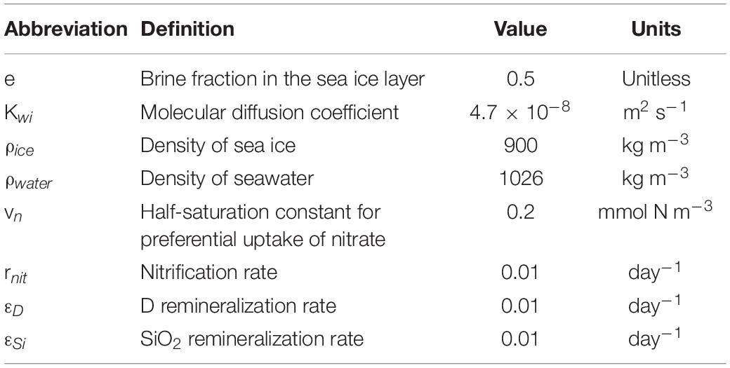
Table 2. List of parameters, corresponding description, and units used in the model for nutrients dynamic.

As for ice algae, the exchange at the sea ice/ocean interface and it depends on rate of change of sea ice thickness $\frac{d{H}_i}{dt}$. This term is positive during sea-ice growth and negative during sea ice melt.

$$\begin{array}{c}{G}_{\mathrm{ice}\mathrm{\_}\mathrm{flux}}\left[ID\right]=\max (0.0,\frac{d{H}_i}{dt})\times \max (0.0,D_f)\times \frac{{\mathrm{\rho }}_{\text{ice}}}{{\mathrm{\rho }}_{\text{water}}}\hfill \\ +\max (0.0,\frac{d{H}_i}{dt})\times \max (0.0,(1-f_{\text{dia}})\times \mathrm{Dia})\times \frac{{\mathrm{\rho }}_{\text{ice}}}{{\mathrm{\rho }}_{\text{water}}}\hfill \\ +\min (0.0,\frac{d{H}_i}{dt}/H_i)\times \max (0.0,[ID])\hfill \end{array}(11)$$

where D_f is fast sinking detritus concentration in mgC m^–3.

Nutrient Dynamics

Inside sea ice, biological communities exist within a complex network of brine channels, extending into the ice layer, with brine volume varying according to the thermohaline characteristics of the ice. Brine volumes are at maximum in the first few centimeters from the ice-ocean interface (Arrigo, 2014; Thomas, 2017), and this is mainly where biological activity is concentrated (Tedesco, 2014). In this present study, we follow an approach suggested in earlier modeling studies (Arrigo et al., 1993; Duarte et al., 2015). Thus, instead of considering a complex brine network dynamic, we assume a bottom layer with biological activity with about 5 cm thickness. The relative brine volume e in this layer is assumed to be 50% (e = 0.5) as suggested by Duarte et al. (2015).

The ice-ocean interface is a dynamic area where exchanges of salt, organic, and inorganic material occur between the two systems (sympagic and pelagic), determining the salinity and nutrient, detritus, and algae concentrations in the sea ice and the water body below. Exchanges occur due to convection, diffusion, ice formation, and ice melting processes (Vancoppenolle et al., 2010; Arrigo, 2014). In the absence of biological activity, it is customary to consider the dynamics of the majority of macro-elements in sea ice following the same dynamical changes as salinity. Meaning that, during the formation of sea ice crystalline lattice impurities and salt are not entrapped in the structure and nutrients and other components are as well rejected in the brines network where they will exchange with the water underneath.

The bulk formulation N_i^bk for each of the aforementioned types of nutrients i is characterized as follows (Belém, 2002; Vancoppenolle et al., 2010):

$$N_i^{bk}=e\times N_i^{br}(12)$$

where N_i^br is the nutrient content for nutrient i in the brine (mmol m^–2) and e is the brine volume fraction (Table 2). Ammonia is an exception to this rule, being entrapped in the crystalline lattice of the ice and expelled to the brine channels (Weeks, 2010; Vancoppenolle et al., 2013). Therefore, the brine concentration of ammonia, unlike the other nutrients, is equal to the bulk mass of ammonia. The rate of change of the respective nutrients in the brine is described as Duarte et al. (2015):

$$\frac{\partial N_{N{O}_3}^{br}}{\partial t}=B{r}_{\text{flux}}+G_{\mathrm{ice}\mathrm{\_}\mathrm{flux}}-\mathrm{\sigma }\left[IA\right]p_{N{O}_3}\frac{\left[N_{N{O}_3}^{br}\right]}{[N_{N{O}_3}^{br}]+[N_{N{H}_4}^{br}]}+r_{\mathit{nit}}\left[N_{N{H}_4}^{br}\right](13)$$

$$\begin{array}{c}\frac{\partial N_{N{H}_4}^{br}}{\partial t}=B{r}_{\text{flux}}+{\mathrm{G}}_{\mathrm{ice}\mathrm{\_}\mathrm{flux}}-\mathrm{\sigma }\left[IA\right]\left(1-p_{N{O}_3}\right)\frac{\left[N_{N{O}_3}^{br}\right]}{[N_{N{O}_3}^{br}]+[N_{N{H}_4}^{br}]}\hfill \\ -r_{nit}[N_{N{H}_4}^{br}]+{\epsilon }_D[D]\hfill \end{array}(14)$$

$$\frac{\partial N_{Si{O}_2}^{br}}{\partial t}=B{r}_{\text{flux}}+G_{\mathrm{ice}\mathrm{\_}\mathrm{flux}}-\mathrm{\sigma }\left[IA\right]+{\epsilon }_{Si}[D](15)$$

$$\frac{\partial N_{P{O}_4}^{br}}{\partial t}=B{r}_{\text{flux}}+G_{\mathrm{ice}\mathrm{\_}\mathrm{flux}}-\mathrm{\sigma }\left[IA\right]+{\epsilon }_D[D](16)$$

The first terms in Eqs 13–16 represent the nutrient transport at the interface due to the diffusion mechanism.

$$B{r}_{\text{flux}}=e\times K_{wi}\times \frac{\partial N_i^{br}}{\partial z}(17)$$

where K_wi is the molecular diffusion coefficient (Jin et al., 2006; Table 2) and dN_i^br/dz is the vertical gradient of the respective nutrient at the ice-ocean interface. The second terms G_{ice_flux} in Eqs 13–16 are either the entrapment of dissolved matter in the ice due to the congelation of water process or the release of nutrients during the ice melt. This entrapment/melting acts on the nutrient bulk. It is defined following the relationship defined as follows (Tedesco and Vichi, 2014):

$$\begin{array}{c}{G}_{\mathrm{ice}\mathrm{\_}\mathrm{flux}}=\max (0.0,\frac{d{H}_i}{dt})\times \max (0.0,N_i^w)\times \frac{{\mathrm{\rho }}_{\text{ice}}}{{\mathrm{\rho }}_{\text{water}}}\times e\hfill \\ +\min (0.0,\frac{d{H}_i}{dt}/H_i)\times \max (0.0,N_i^{bk})\hfill \end{array}(18)$$

where N_i^w is the water concentration of nutrient i (mmol m^–3). For ammonium, during the congelation process the quantity is not divided by the brine fraction due to the entrapment into the crystalline lattice as well in the brine. The third terms of the Eqs 13–16 are the uptake of nutrients by ice algae. Here p_NO3 in Eqs 13 and 14 differentiate the uptake of nitrate from that of ammonium based on Mortenson et al. (2017):

$$p_{N{O}_3}=\frac{v_n}{v_n+[N_{N{H}_4}^{br}]}(19)$$

where v_n is the half-saturation constant for preferential uptake of nitrate (Table 2). The fourth terms in Eqs 13 and 14 are the nitrification rate, which is fixed as constant here (Table 2). The last terms in Eqs 14–16 represent the remineralization process from the detritus pool in sea ice. The remineralization rate is constant (Table 2).

Biogeochemical Pelagic Modifications

The ocean biogeochemical model ECOSMO includes 13 state variables describing three nutrient cycles (NO₃, NH₄, SiO₂, and PO₄), two phytoplankton groups (diatoms, flagellates), two zooplankton groups (mesozooplankton and microzooplankton), oxygen, biogenic opal, detritus (fast and slow), and dissolved organic matter. In the here used setup, the benthic system is included in the model formulation consisting of three state variables, of which each corresponds to a respective nutrient pool in the sediment (nitrogen, silicate, and phosphate). Model equations and parameterization are described in detail elsewhere (Daewel and Schrum, 2013; Daewel et al., 2019). To study the Arctic system and the sympagic-pelagic-benthic interactions, some changes have been made. These changes are explained in the section below. In particular we split the detritus group into a fast (D_f) and a slow (D_s) sinking class. Similar to diatom entrapment into sea ice, during the melting phase not all the ice algae are transferred to the diatom pool but only a fraction, corresponding to the surviving algae. The same fraction f_dia as for the entrapment is used. The remaining part is added to the fast sinking detritus pool. Additionally, the sea-ice detritus is released into the fast sinking detritus pool in the water column during ice melt. The reaction equations for two detritus groups are given as:

$$\begin{array}{rcl}{R}_{D_f}& & =(1-a_{\mathrm{dom}})R_{D_f}^{+}-R_{D_f}^{-}+[{\lambda }_{s2d}{C}_{S{E}_1}\\ & & {-{\lambda }_{d2s}{C}_{D_f}/dz]}_{z=\mathrm{bottom}}\end{array}(20)$$

$$R_{D_f}^{+}=G_{\mathrm{ice}\mathrm{\_}\mathrm{flux}}[ID](21)$$

$$R_{D_f}^{-}=\sum _{i=1}^2{C}_{Z_i}{G}_i\left(C_{D_f}\right)+{\mathrm{\epsilon }}_D\left(T\right)C_{D_f}(22)$$

$$\begin{array}{rcl}{R}_{D_s}& & =(1-a_{\mathrm{dom}})R_{D_s}^{+}-R_{D_s}^{-}+[{\lambda }_{s2d}{C}_{S{E}_1}\\ & & {-{\lambda }_{d2s}{C}_{D_s}/dz]}_{z=\mathrm{bottom}}\end{array}(23)$$

$$\begin{array}{rcl}{R}_{D_s}^{+}& & =(1-{\gamma }_1)(\sum _{i=1}^2{C}_{Z_i}\sum _{j=2}^2{G}_i\left(C_{P_j}\right)+G_2\left(C_{Z_1}\right))\\ & & +(1-{\gamma }_2)\sum _{i=1}^2{C}_{Z_i}{G}_i\left(C_{D_s}\right)\\ & & +\sum _{j=1}^2{m}_{P_j}{C}_{P_j}+\sum _{i=1}^2{m}_{Z_i}{C}_{Z_i}\end{array}(24)$$

$$R_{D_s}^{-}=\sum _{i=1}^2{C}_{Z_i}{G}_i\left(C_{D_s}\right)+{\mathrm{\epsilon }}_D\left(T\right)C_{D_s}(25)$$

where, T is the temperature in °C and z the depth in m. C_X is biomass of the state variable of the X in mgC m^–3, where X represents P_j [phytoplankton group with j = 1, 2 denotes the phytoplankton type (1: diatom, 2: flagellate)]; Z_i [zooplankton group with i = 1, 2 denotes the zooplankton type (1: micro-, 2: meso-zooplankton] and SE₁ is the sediment group representing the sediment carbon pool. G_i–1,2 is the zooplankton grazing rate. A sensitivity analysis (not included in the results) on the different sinking speed for the fast sinking detritus group showed that a sinking speed of 50 m d^–1 leads to the best representation of the ecosystem dynamics. This value has also been chosen in earlier modeling studies by Lavoie et al. (2005) and Mortenson et al. (2017). The parameters values for Eqs 18–23 are given in Table 3. Additionally, we added a temperature dependence to the phytoplankton growth rate following an exponential function as described by Eppley (1972):

$$f_T=e^{T_{\text{lim}}\times T}(26)$$

TABLE 3

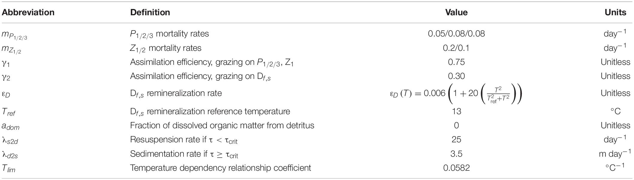
Table 3. List of parameters, corresponding description, and units used in the model for pelagic dynamic.

where, T is the ambient temperature in°C and T_lim is the reference temperature (Table 3).

Light

Light is one major factor controlling growth of both sea-ice algae and phytoplankton in the water column. Light that penetrates in and through the ice reaching the sea-ice algal communities depends on the snow and ice thickness following the Beer–Lambert law as Castellani et al. (2017):

$$I(H_{\text{ice}},H_{\text{snow}})=I_0\left(1-{\mathrm{\alpha }}_{(\mathrm{ice},\mathrm{snow})}\right)C_0{e}^{-k_{\text{ice}}{H}_{\text{ice}}-k_{\text{snow}}{H}_{\text{snow}}}(27)$$

where I₀ is the shortwave incoming solar radiation, α is the albedo of the surface component ice or snow, C₀ is the fraction of incoming radiation absorbed in the first centimeters of snow or ice layer, k_ice and k_snow are the ice and snow attenuation coefficient respectively and H_ice and H_snow are the ice and snow thickness, respectively. All parameter values and units are referred in Table 4.

TABLE 4

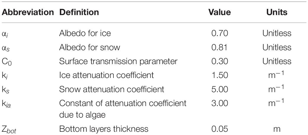
Table 4. List of parameters, corresponding description, and units used in the model for light calculation (most of parameters values come from Castellani et al., 2017).

Light available for phytoplankton in the water column below the ice depends on the snow and ice thickness but also on the ice algae concentration. In a given grid cell, however, the available light for primary production in the water column is additionally determined by what fraction of the area is covered by ice A (Slagstad et al., 2015). Light intensity reaching the water column below ice is expressed as:

$$\begin{array}{rcl}I(H_{\mathrm{ice}},H_{\mathrm{snow}},Z_{\mathrm{bot}})& & =I_0(1-{\alpha }_{\left(\mathrm{ice},\mathrm{snow}\right)})\\ & & C_0{e}^{-k_{\mathrm{ice}}{H}_{\mathrm{ice}}-k_{\mathrm{snow}}{H}_{\mathrm{snow}}-k_{\mathrm{ia}}{Z}_{\mathrm{bot}}\left[IA\right]}\end{array}(28)$$

where Z_bot is the thickness of the biologically active bottom sea ice layer. The total light available in a grid cell is then given by:

$$I_{\text{tot}}=A\times I(H_i,H_s,Z_{\text{bot}})+\left(1-A\right)\times I_0(29)$$

Numerical Experiments and Sensitivity Analysis

With the 1D model setup we performed numerical experiments to understand primary and secondary production in the Barents Sea. Even though the Barents Sea is one of the most productive areas in the Arctic Ocean it features a high spatial variability in ecosystem productivity with less production in the northern than in the southern areas (Sakshaug, 1997; Dalpadado et al., 2014). To address the spatial dynamics, we ran simulations at three separate locations (Figure 2) that differ in ice dynamics and environmental conditions. The southernmost station was located in an area where the ocean is free of ice all year round (SBS: 39.25 E; 71.41 N). A second station in the center of the Barents Sea (MBS: 38.58 E; 76.44 N) represents the area with a seasonal cycle in ice coverage where the ocean is free of ice during late summer. The third station represented the area with year-round ice coverage, located in the northern Barents Sea (NBS: 35 E; 81.6 N). All the simulations were performed with a 30 min time step and daily means were provided for analysis. As initial concentration for the modeled state variables for ice algae, diatom, flagellate, microzooplankton, mesozooplankton, and two detritus pools very small values were chosen (0.0, 0.1, 0.1, 0.01, 0.01, and 0.05 mgC m^–2, respectively) for all three stations. The state variables for nitrate, ammonium, phosphate, and silicate were initialized based on observed winter concentrations in the central Barents Sea (Reigstad et al., 2002; Sakshaug et al., 2009) (10.5, 2, 0.8, and 4.5 mmol m^–3).

FIGURE 2

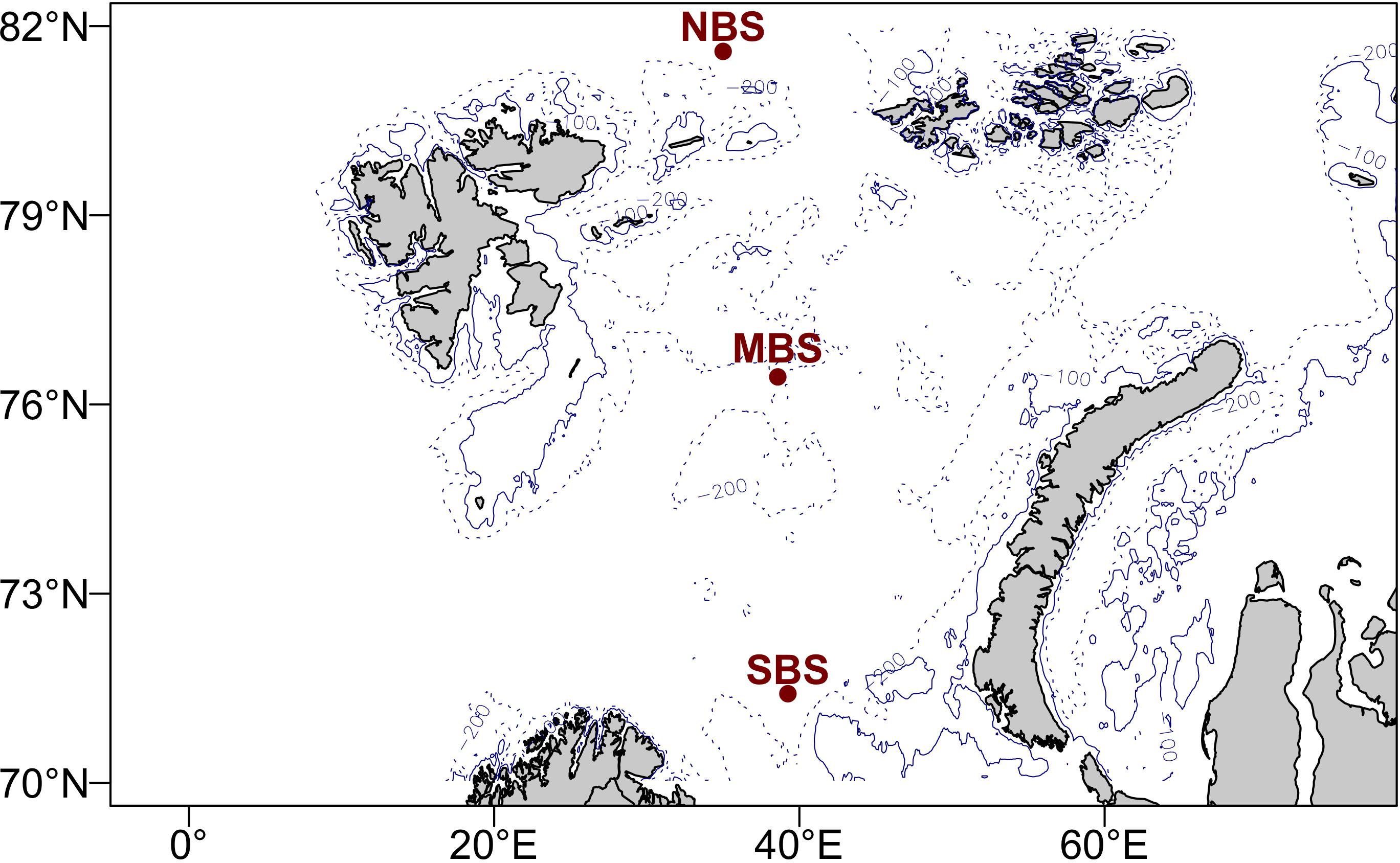
Figure 2. Map of the Barents Sea area. Red dots indicate the three stations where environmental forcing are extracted to run experimental simulation. NBS means north Barents Sea station, MBS means central Barents Sea station, and SBS means south Barents Sea station.

We performed three sets of scenarios to evaluate the primary and secondary production in the Barents Sea area at different spatial and temporal scale. The first set of experiments was designed to understand the response of the pelagic production system to implementation of the sympagic ecosystem dynamics in the model. These scenarios were run at MBS location during 1997. In this first set of experiments, we ran the same setup (i) including all the biogeochemical components and interaction between the sympagic and the pelagic systems (fullBGC scenario), (ii) neglecting the biogeochemical interaction between the sympagic and the pelagic system but including the sea ice physics (noBGC scenario), and (iii) neglecting the sea ice completely (noICE scenario), which allowed us to dissociate the role of the sea ice presence itself and the role of the sea ice biogeochemistry on the pelagic system. This last experiment also explores the ice free environment, which is expected in the next decades considering climate induced sea ice retreat (Onarheim and Årthun, 2017).

The second set of scenario experiments described the spatial variability of the primary and secondary production at three stations (NBS, MBS, and SBS) following a north-south gradient.

The third set of scenario experiments addressed the interannual variability of the primary and secondary production at the MBS station. We ran each simulation for a 10 years’ time period (1990–1999), where the first 2 years were considered as spin-up period and were disregarded for analysis.

Since the Arctic ecosystem is difficult to access and data on parameters relevant for the sympagic ecosystem are sparse, we additionally performed a sensitivity study to investigate the models’ response to some of the most uncertain parameters in the ice-ecosystem formulation. The proportion of phytoplankton entrapped in the ice during freezing determines the initialization of the sea-ice algae and thus consequently ice algae biomass but is hardly measurable and thus difficult to identify. Some evidence shows that ice algae stem from different sources (multi-year ice, pelagic system, benthic system; Syvertsen, 1991; Ratkova and Wassmann, 2005; Werner et al., 2007; Olsen et al., 2017). But it remains unclear how much exactly originates from the pelagic system and finally survives inside the ice. On the other hand, the proportion of ice algae released into the water during the sea ice melt contributes to the algal biomass in the water column and can be used by zooplankton as a valuable food source (Michel et al., 1996; Søreide et al., 2006, 2013). Moreover, some studies highlight the potential of some ice algae species to seed phytoplankton production during the ice melt (Haecky et al., 1998; Galindo et al., 2014; Szymanski and Gradinger, 2016). Through a sensitivity analysis, we evaluated the impact of the amount of phytoplankton entrapped in sea ice on ice algae phenology and, of the amount of ice algae released to the pelagic system on the primary and secondary production. We ran four scenarios for this experiment:

1. control run: 100% of diatoms entrapped is transferred into the ice algae pool and 100% of ice algae is release to the diatom pool;

2. 75% of the diatoms entrapped are transferred to the ice algae pool while the remaining 25% are transferred to the ice detritus pool and, 75% of the ice algae released are transferred in the diatoms pool while the remaining 25% are transferred to the pelagic fast sinking detritus pool;

3. where the proportion of algae:detritus is 50:50%;

4. where the proportion of algae:detritus is 25:75%.

The main assumption of the 1D modeling approach described here is that lateral advection in both the ice and water layers is negligible compared to other fluxes. We used forcing data retrieved from outputs of a 3D hydrodynamic model – which includes advection – to define the seasonality of temperature, vertical mixing, and ice properties. However, the 1D model itself does account for net lateral fluxes of state variables at the given location. This limitation does not invalidate the approach as deployed in this article for exploring hypotheses on the linkage between sympagic-pelagic-benthic systems provided the deployment locations are chosen carefully to avoid areas with strong horizontal gradients in the model variables so that advection is of secondary importance. However, it could become an issue for interpretation of responses to climate change. Climate warming is not only accompanied by loss of sea ice, but also by changes in wind patterns, water mass characteristics and circulation (Skagseth et al., 2020). These could change net horizontal fluxes, especially of ice at our study sites in the Barents Sea (Kimura and Wakatsuchi, 2001; Koenigk et al., 2009; Kwok, 2009). Hence advection could become a significant term in the rate of change of ice algae biomass at model locations. Thus, in the next step of our work we will apply the model in a fully coupled 3D biological-physical model to account for the dynamics nature of the system. This will additionally account for sea ice dynamic forced by the atmospheric conditions, which has clear implications for both sympagic as well as pelagic productivity.

Results and Discussion

Role of Sympagic System: Implementation, Verification, and Sensitivity

In Figure 3 we show the seasonal variations of estimated ice algae dynamics (fullBGC scenario) and the related external and internal properties. The results show that ice algae growth started slowly at the beginning of March as soon as sufficient light became available (Figure 3E), and prevailed until mid-June when biomass started to decrease (Figure 3C) controlled by both ice melting (Figures 3A,B) and grazing by pelagic zooplankton. The ice algae growth dynamic was characterized by three blooms. The two first occurred in early and mid-May, both followed by a sharp decrease of biomass due to two melting events, generating a strong ice algae release (Figure 3B). A third bloom, which was the most important, occurred in mid-June (Figure 3C), during which the biomass increased up to 378 mgC m^–2 with a maximum daily ice algae production rate about 89 mgC m^–2 d^–1. Our biomass estimates were consistent with data from field measurement in the Barents Sea area (69–620 mgC m^–2; Tamelander et al., 2009) and in the Arctic region (3–460 mgC m^–2; Gosselin et al., 1997). The results on daily ice algae production rate, however, appear to be higher than measured production rates in the northern Barents sea (0.16–55 mgC m^–2 d^–1; Hegseth, 1998; McMinn and Hegseth, 2007). On the other hand, our results showed low biomass of ice algae when compared with data from Rózañska et al. (2009) and Fernández-Méndez et al. (2018), who reported ice algae biomasses up to 2250 mgC m^–2, indicating that our model might underestimate ice algae biomass. The abiotic environment (e.g., light, ice, and snow thickness) strongly influences the daily ice algae production rate. These environmental conditions vary strongly in the Barents Sea both spatially and temporally, which can explain these differences between model results and observations, particularly since our environmental forcing is only representative for one specific location. Moreover, we only consider ice algae originating from entrapment of pelagic algae, which neglecting ice algae advection from other area. As this provide a relatively small quantity of algae it impacts the growth of biomass and might explain the slow growth between March and May, and the potentially too low ice algae biomass. Nonetheless, over the large existing range of measured and simulated production rates (from 0.16 to 100 mgC m^–2 d^–1; Clasby et al., 1973; Mortenson et al., 2017) our simulated values are well in the range of previously reported production rates and our daily production rates appear acceptable.

FIGURE 3

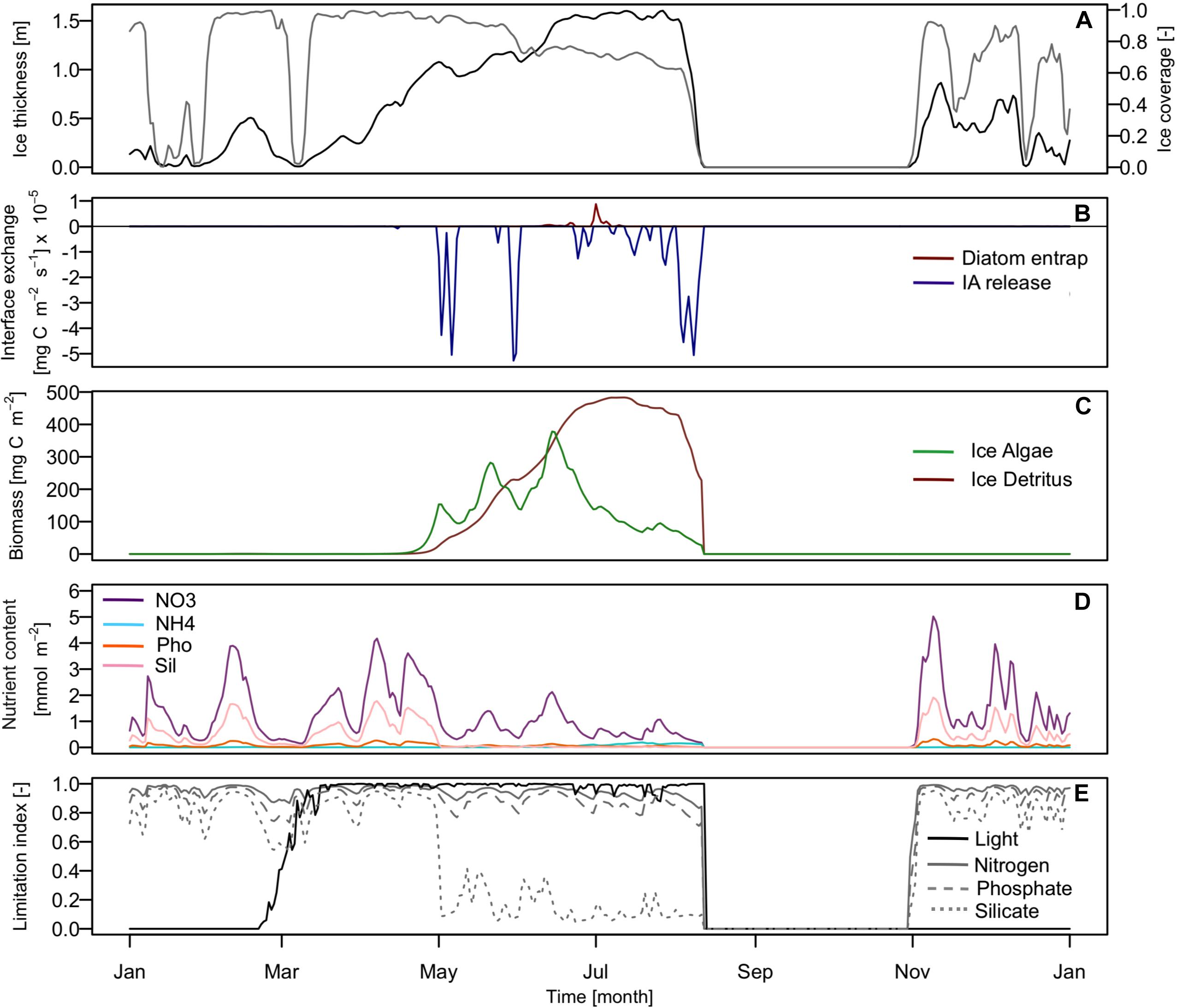
Figure 3. Seasonal variation in the environmental forcing (A) of ice thickness (black) and ice coverage (gray) in 1997; (B) diatoms/ice algae flux at the ice-ocean interface. (Red line represents the quantity of diatoms entrap into the sympagic system and the blue line represents the quantity of ice algae released into the pelagic system.); (C) the ice algae (green) and detritus in ice (red) biomass; (D) integrated nutrient content in the sea ice: nitrate (NO₃: purple), ammonium (NH₄: light green), phosphate (Pho: orange), and silicate (Sil: pink); (E) light (black) and nutrients (gray) ice algae growth limitation index. Nitrogen (solid), phosphate (dashed), and silicate (dotted) are represented.

The simulated ice algae bloom dynamic was not nutrient limited in our scenario (Figure 3E), even though the silicate concentration decreased sharply during the bloom event, it never became limiting (Figures 3D,E). Our simulations show two strong melt events during the ice algae bloom period which removed a substantial amount of ice algae biomass from the ice, which also reduced the nutrient requirements in the ice. In addition, the ice bottom layer at the ocean interface is highly dynamic and nutrients can be replenished by convective mixing (Vancoppenolle et al., 2010). This is in compliance with findings from Werner et al. (2007), who showed that ice algae do not appear to be limited by nutrients in the Barents Sea. The Barents Sea is a shallow area and is significantly influenced by winds and tidal mixing (Sundfjord et al., 2007). Hence nutrients are abundant and not generally a limiting factor for ice algae as also shown by Tamelander et al. (2009). The total annual production of the simulated ice algae was about 2.44 gC m^–2, which represented about 3.8% of the total primary production. This fraction is in the lower part of the range of the observations previously reported for the whole Arctic (3–57%; Gosselin et al., 1997). According to Sakshaug (1997) and Hegseth (1998) who reported estimated total annual production respectively around 6 and 7% of the total primary production in the northern Barents Sea, our total production estimation appeared to be slightly underestimated but reasonable.

In order to assess the role of the sympagic system on the overall ecosystem dynamics, we performed three numerical experiments to separate the impacts of the physical and biological forcing. The results are presented in Figure 4 for the fullBGC (Figures 4A,D,G,J), the noBGC (Figures 4B,E,H,K) and the noICE scenario (Figures 4C,F,I,L). Scenario explanations are given the methods section. The results highlight how the sympagic system generates important changes in the whole ecosystem by modifying the phytoplankton and zooplankton phenology.

FIGURE 4

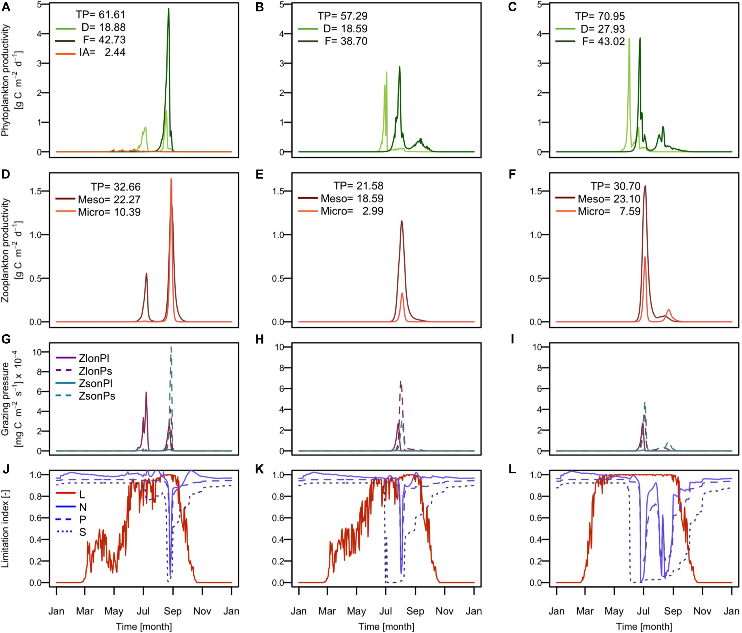
Figure 4. Simulated sympagic and pelagic primary and secondary production, predation pressure of zooplankton on phytoplankton and nutrient and light growth limitation in the surface layer (4 m depth) for full coupling experiment (A,D,G,J), physical coupling experiment (B,E,H,K), and free ice experiment (C,F,I,L). Time series of (A–C) primary production rates of ice algae (IA: orange), diatoms (D: light green), and flagellates (F: dark green), (D–F) secondary production rates of mesozooplankton (Meso: dark red) and microzooplankton (Micro: orange), (G–I) grazing rates of large and small zooplankton on large and small phytoplankton, and (J–L) growth limitation index for light (solid orange), nitrogen (solid blue), phosphate (dashed blue), and silicate (dotted blue). In the legend (A–F) are indicated the annual production in gC m² for total pelagic production (TP), diatoms (D), flagellates (F), ice algae (IA), mesozooplankton (Meso), and microzooplankton (Micro). In the legend (G–I) are indicated large zooplankton grazing rate on large phytoplankton (ZlonPl), large zooplankton grazing rate on small phytoplankton (ZlonPs), small zooplankton grazing rate on large phytoplankton (ZsonPl), and small zooplankton grazing rate on small phytoplankton (ZsonPs). In the legend (J–L) are indicated light limitation (L), nitrogen limitation (N), phosphate limitation (P), and silicate limitation (S) at the surface layer.

What we generally can see is that implementing ice biogeochemistry in the model formulation strongly impacts the dynamics of the pelagic ecosystem, both with respect to magnitude and timing of the different components. Most importantly, we found major differences in the dynamics of diatoms and zooplankton. In the fullBGC scenario, when the sympagic system was fully implemented, the model estimated two diatom blooms during the season (Figure 4A), while only one spring bloom was simulated in noBGC. The first bloom occurred in July in both scenarios, partly under ice, when the ice coverage started to decrease, allowing better light conditions in the water column. In case of fullBGC, this bloom was not limited by nutrients but instead controlled by zooplankton grazing (Figures 4G,J). In the noBGC scenario, on the other hand, this first diatom bloom developed until silicate became limiting. The major process leading to this difference was that generally the zooplankton benefits from feeding on ice algae prior to the first diatom bloom, leading to relatively high zooplankton biomasses early in the season (Figure 4D). Consequently, zooplankton and phytoplankton maximum biomass occurred at the same time (Figures 4A,D), which systematically modified the overall system dynamics. Therefore, silicate remained in the water column allowing a second diatom bloom in August during full open water condition following the ice break-up. Zooplankton grazing on ice algae, in the ice and in the water column just after being released, appears one of the most important links between the pelagic and sympagic component of the ecosystem leading in our results to a general increase in zooplankton biomass. This important link has earlier been reported on the basis of field observations (Stretch et al., 1988; Runge and Ingram, 1991; Werner, 1997; Juul-Pedersen et al., 2008). Observations indicate that the grazing on ice algae is partly used by female copepods to mature their gonads and produce eggs (Søreide et al., 2010; Durbin and Casas, 2014). In this case, there is an increase in biomass due to egg production. But because eggs do not feed directly on phytoplankton during their development and only participate in phytoplankton consumption later in the season after hatching, the control of our first phytoplankton bloom by the zooplankton grazing could potentially be overestimated. More investigations are necessary here to accurately understand the direct role of ice algae on zooplankton dynamics and vice versa. Nonetheless, the interaction between the pelagic zooplankton and ice algae remains an important process as it determines the fitness of these zooplankton species and includes other species that use ice algae such as amphipods and krill.

The flagellate bloom occurred after the ice break-up at the same time as the second diatoms bloom (Figure 4A) but with a much higher biomass. Flagellates generally dominated the primary production with a total annual production about 42.73 gC m^–2, which represent around two thirds of the total pelagic primary production (61.61 gC m^–2). Previous studies estimated annual primary production for the Barents Sea to be between 20 and 200 gC m^–2, depending on the area, with estimates around 76 gC m^–2 in the central Barents Sea (Luchetta et al., 2000; Sakshaug et al., 2009), which supports our model estimates. The high flagellate biomass results from the fact that the diatoms are mainly controlled by zooplanktonic grazing. This leads to relatively high nutrient concentrations (Figure 4J) and consequently allows a strong flagellate bloom in the fall. Also, for mesozooplankton a second maximum follows the spring maximum in July and is closely related to the diatom dynamics. Microzooplankton, on the other hand, followed the flagellate’s dynamic with a unique peak by the end of summer. Mesozooplankton dominated the secondary production.

In Figure 5, we showed differences between the fullBGC and the noBGC scenario in the vertical biomass profiles of the two detritus groups (Figure 5A: fast and Figure 5B: slow sinking rate). These results indicate a lower biomass of slow sinking detritus during summer (Figure 5B) when the sympagic system is coupled to the pelagic ecosystem, related to a smaller summer diatom bloom in the fullBGC scenario. This was followed by a second strong detritus production in autumn, which was exported to the benthic system in late autumn, and which corresponds to the strong flagellate production. Direct export of ice algae to the benthic system happened at the end of summer when ice melts. We observed a contribution of the fast sinking detritus group in September with a slightly higher export to the benthic system in the fullBGC scenario compared to the noBGC scenario (Figure 5A). It has already been shown that ice algae contributes to the export of matter to the benthos due to the fast sinking rate and it represents a valuable resource for benthic organisms early in the season (Søreide et al., 2013; Schollmeier et al., 2018). Due to the forcing data we used, the simulated ice break-up occurred late in the season at mid-June and we did not observe a spring contribution of ice algae to the benthos as was showed in previous studies (Boetius et al., 2013; Szymanski and Gradinger, 2016). However, our results pointed out that the ice algae are exported rapidly to the benthos and earlier than the phytoplankton in the productive season (Figure 5). In addition, our results highlight the indirect contribution to detritus export by changes in zooplankton dynamics (Figure 5B). Because of the feeding process on ice algae, zooplankton developed earlier and participated in an increase in the slow sinking detritus biomass. The results indicate temporal changes on the export of detritus biomass to the benthic system when sympagic biogeochemistry is included. The sympagic system therefore does not only play a role in pelagic dynamics but also influences both the amplitude and timing of detritus export to the benthic system. Here, we additionally hypothesize that the indirect contribution due to the zooplankton feeding on the ice algae is as important for the timing and magnitude of material export to the benthic system.

FIGURE 5

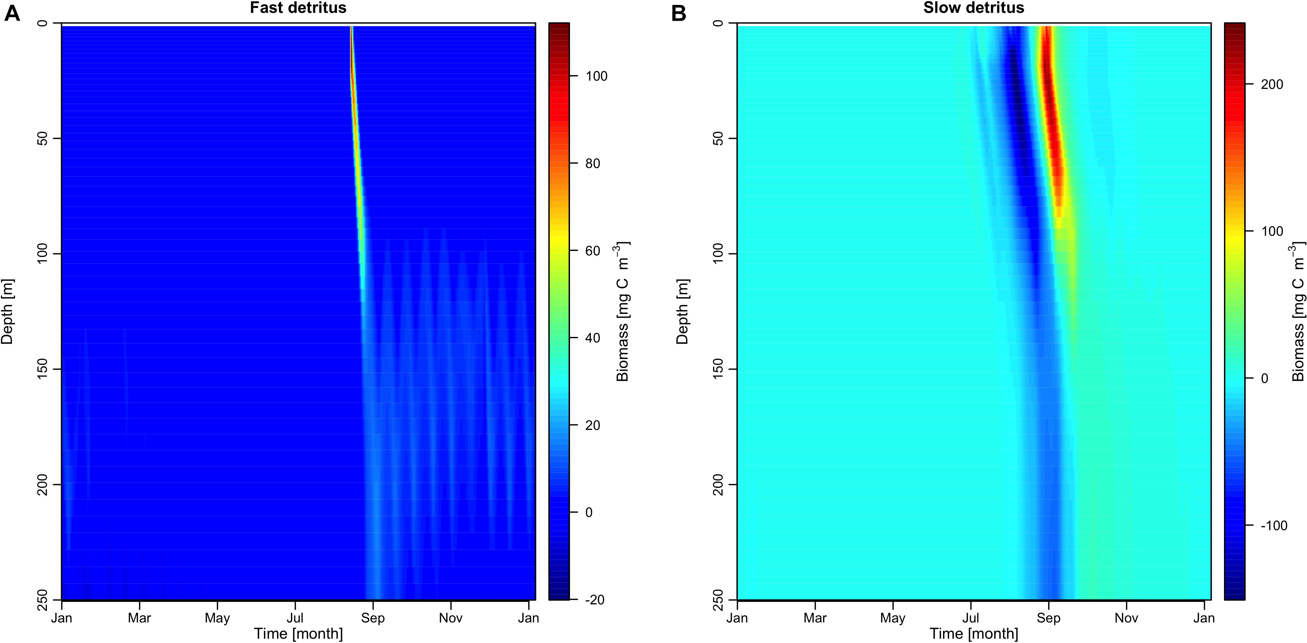
Figure 5. Vertical profile of difference in biomass concentration between full coupling experiment and physical coupling experiment for the fast sinking rate detritus group (A) and the slow sinking rate detritus group (B).

The noICE scenario shows similar dynamics to the noBGC scenario. The main difference observed is an earlier onset of spring bloom production with about one-month time difference (Figures 4B,C). This is due to the absence of ice cover leading to sufficient light conditions earlier in the year (Figures 4K,L). The other major difference is the increase of the total annual primary and secondary productivity in the noICE scenario. The structure of the ecosystem groups does not change between these two scenarios suggesting that the presence of ice only as a physical barrier does not seem to influence pelagic ecosystem functioning. Differences between fullBGC and noICE scenarios, i.e., earlier primary production and higher primary production, reflect changes expected for the Arctic region regarding an ice decrease. These changes are further discussed in the section Spatial variability in the Barents Sea, environmental drivers and ecosystem dynamics.

Results of the sensitivity analysis (Figures 6A,B) showed that the proportion of phytoplankton entrapped in the ice influenced slightly the total ice algae production with a change of about 0.25 gC m^–2 y^–1 between the 100 and 25% numerical experiments, which represent a decrease of about 10% for an entrapment proportion decrease of 75%. The sensitivity experiments did not indicate any changes in ice algae production in terms of timing and amplitude of the maximum growth rate. This principally resulted from the minimum threshold implemented in our model to allow a minimum proportion of ice algae to survive during winter in the ice when conditions are not favorable for growth. This assumption was made because the fate and origin of ice algae during winter remains poorly understood. Different hypotheses were suggested previously including the existence of resting cysts or spores, metabolism adaptation to low light, facultative heterotrophy, or origin of algae in the ice from nearby multi-year ice (Syvertsen, 1991; Niemi et al., 2011; Kauko et al., 2018). Even though the total amount of ice primary production changed only slightly, we found that the magnitude of the initial bloom in May was decreased by almost 50% when only 25% of the entrapped algae were used for production.

FIGURE 6

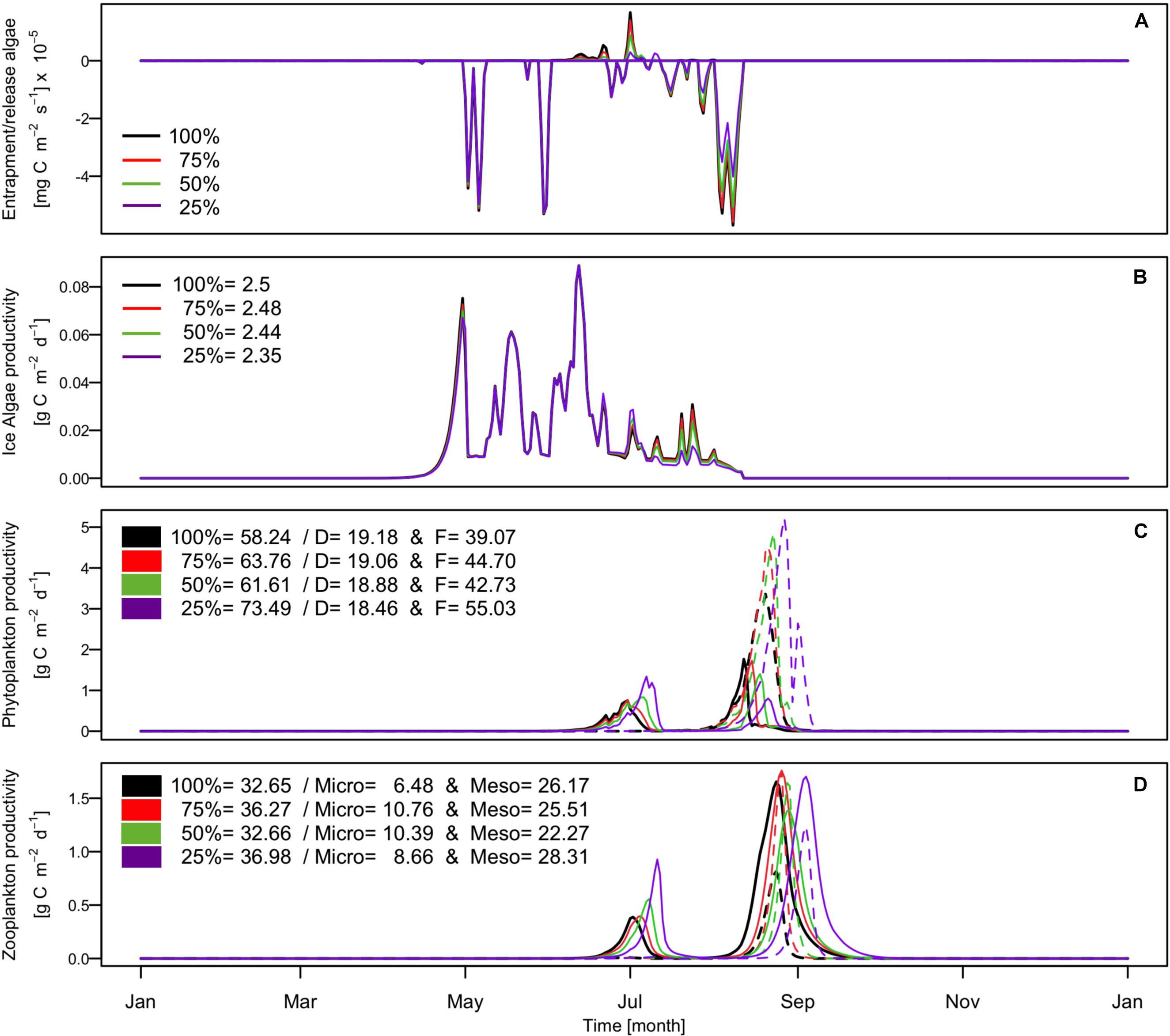
Figure 6. Simulated time series of (A) diatoms/ice algae flux at the ice-ocean interface; (B) production rates of ice algae; (C) production rates of phytoplankton including diatoms (D: solid line) and flagellates (F: dashed line), and (D) production rates of zooplankton including mesozooplankton (Meso: solid line) and microzooplankton (Micro: dashed line). Black color presents result for the 100% experiment, red color for the 75% experiment, green color for the 50% experiment, and purple color the 25% experiment. In the legend (B–D) are indicated the annual production in gC m^–2 for ice algae, phytoplankton including diatoms production (D) and flagellates production (F) and zooplankton including microzooplankton (Micro) and mesozooplankton (Meso).

Although variations in phytoplankton entrapment did not show a prominent effect on the sympagic production, the modeled pelagic system showed a clear response to the amount of ice algae released into the sympagic system during ice melt (Figures 6C,D). First, our results indicate that released ice algae seeded the diatoms blooms, both under ice and during the ice break-up. This is one of the main assumptions made in our approach. The hypotheses about the ice algae seeding are divergent and controversially discussed in the scientific community, because evidence is not clear. Some field samplings highlight that ice algae contribute to the start of the phytoplankton bloom, due to some species overlapping in both the sympagic and pelagic communities (Haecky et al., 1998; Lizotte, 2001; Mangoni et al., 2009). Contradictory field studies have indicated that ice and pelagic algae communities are distinct and that ice algae apparently do not seed phytoplankton blooms (Riebesell et al., 1991; Mundy et al., 2014). Our results showed that, under the condition of ice algae seeding, the proportion of ice algae released into the diatom pool has consequences for the phenology of the diatoms, with an earlier peak biomass the more ice algae are released. This consequently also results in a modified phenology of the secondary production. The maximum difference in peak bloom timing for the two most extreme experiments (100 and 25%) was about 1 week, both for the under-ice bloom and the late summer bloom. The results thereby showed that the peak production occurred later the less important the ice algae seeding is for the overall diatom biomass. This estimated change in diatom phenology systematically modified the primary producers’ dynamics. The associated environmental conditions, such as temperature, ice cover, and available light, in the water column change slightly within this 1-week period. This influences the growth rate of the diatoms such that, although the seeding of diatoms was lower, it led to a shorter bloom with higher peak biomass. After the ice break-up flagellates developed quickly, limiting the diatom bloom. Because ice algae seed the diatom blooms it allowed them to bloom earlier at the ice break-up. Therefore, the smaller the ice algae release is, the weaker the second bloom and the greater the flagellate’s production. The difference in total flagellate production between the 100 and 25% experiments was an increase of 40.8%. In light of our results and also model results published by Tedesco et al. (2012) and Jin et al. (2007) ice algae seeding appears to be a key process in the Arctic marine ecosystem dynamics and further investigations should be done in order to decrease uncertainties about this process. Especially as Lizotte (2001) highlighted, climate change can alter and modify algae communities and consequently potentially change the contribution of ice algae to the phytoplankton bloom.

The sensitivity analysis again highlights the importance of clarifying the current parameterization of sympagic components and the exchanges with the pelagic components underneath. Despite ice algae representing a small proportion of the total primary production, we showed that its contribution to the phenology of all the pelagic groups is significant. The results also suggest important changes in the Arctic pelagic structure of planktonic communities might be related to ice algae changes, as already suggested before for copepods in an earlier study (Tedesco et al., 2019). Indeed, there is evidences that females of C. finmarchicus and C. glacialis, when barely out of diapause, benefit from feeding on ice algae to maturate their gonads and produce eggs (Hirche and Kosobokova, 2003; Søreide et al., 2010; Leu et al., 2011). Although, the factors of entry and exit in a diapause state remain not well identified, some evidence about a mismatch between the presence of individuals at the surface and algal bloom have already been highlighted, showing significant consequences for fitness and next generations of these species (Dezutter et al., 2019). Diapause behavior is not yet a part of our model formulation and should be integrated in future work to identify more accurately the planktonic phenology in the Arctic system as modeling work of Pourchez (2018) showed for the Beaufort Sea. We previously discussed a possible model artifact of zooplankton controlling the first phytoplankton bloom due to an earlier growing phase feeding on ice algae. If we consider that a significant zooplankton biomass migrates from the bottom to the surface at springtime, it seems realistic that such a grazing control takes place. It could also help to explain the second phytoplankton bloom in autumn, when naturally zooplankton migrates back to the bottom and relieves the grazing pressure (Pourchez, 2018). Identification of these key parameters becomes all the more urgent in the context of rapid climate change in order to properly understand and manage the near future Arctic ecosystem.

Spatial Variability in the Barents Sea, Environmental Drivers and Ecosystem Dynamic

The Barents Sea area exhibits strong seasonal contrasts as well as high spatial variability, as illustrated in Figure 7 regarding the light availability at the ocean surface (Figure 7A) and the sea ice thickness (Figure 7B). This high variability in environmental conditions results in very different ecosystem dynamics and follows mainly a south-north gradient related to temperature and ice cover (Figures 8, 9). For the northernmost station (NBS), which is covered by ice all year round, our results showed the lowest productivity, with a total annual primary production of 2.86 gC m^–2 yr^–1, while at the central and southernmost location our model estimated 64.05 gC m^–2 yr^–1 and 96.89 gC m^–2 yr^–1, respectively (Figure 8). This was due to the presence of a thick ice coverage in the north leading to low light availability at the ice-ocean interface. Our results are consistent with field observations provided by Sakshaug et al. (2009), who estimated that primary production varied from <20 to 200 gC m^–2 yr^–1 over the Barents Sea. Even though ice algae production was relatively small in the north when compared to the central Barents Sea area, it was more important for the overall productivity in the region representing around 42% of the total primary production at this location. In contrast, in the central Barents Sea the ice algae accounted only for 3.8% of the overall primary production (Figure 8A). Light conditions not only determined the magnitude but also the phenology of the productivity resulting in an onset of spring diatom bloom in the beginning of June in the southern Barents Sea, beginning of July in the central Barents Sea, and middle of August in the northern station (Figure 8B). A second diatom bloom developed only in the central Barents Sea area in the middle of August when ice break-up allowed more favorable light conditions. Flagellates bloomed twice (end of June and beginning of August) in the south, whereas in the central Barents Sea only one bloom occurred in the middle of August. Environmental conditions at the northern location are generally not favorable for primary production and flagellates were outcompeted by diatoms. In contrast, flagellates dominated the primary production in the south and central part of the Barents Sea by around two thirds.

FIGURE 7

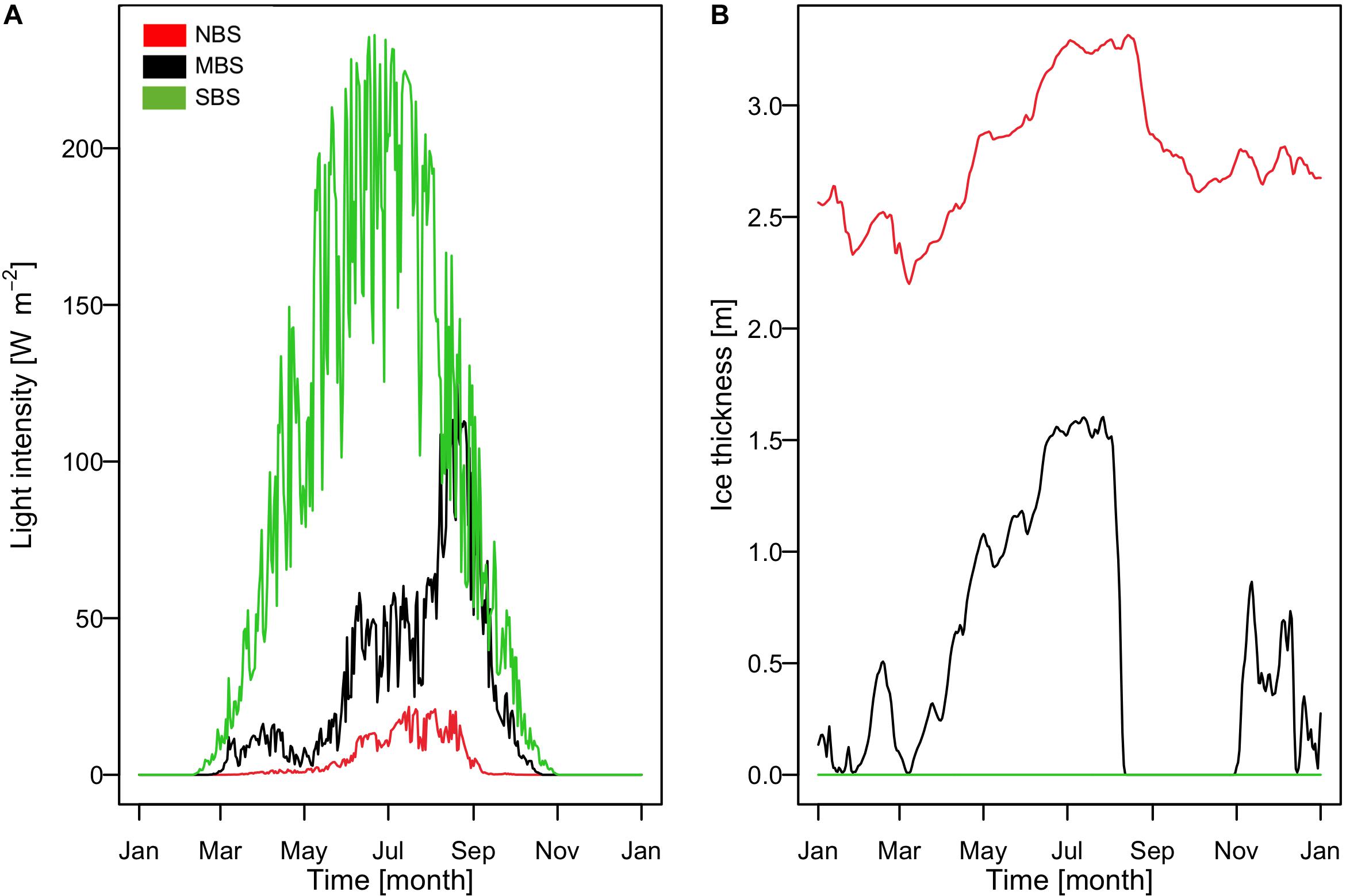
Figure 7. Simulated time series of (A) light intensity (W m^–2) at the ocean surface (includes ice and ice algae attenuation) and (B) extracted sea ice thickness (m) forcing. Black color presents result for the central Barents Sea station over the 1997, red color for the north Barents Sea station over the 1997, and green color for the south Barents Sea station over the 1997.

FIGURE 8

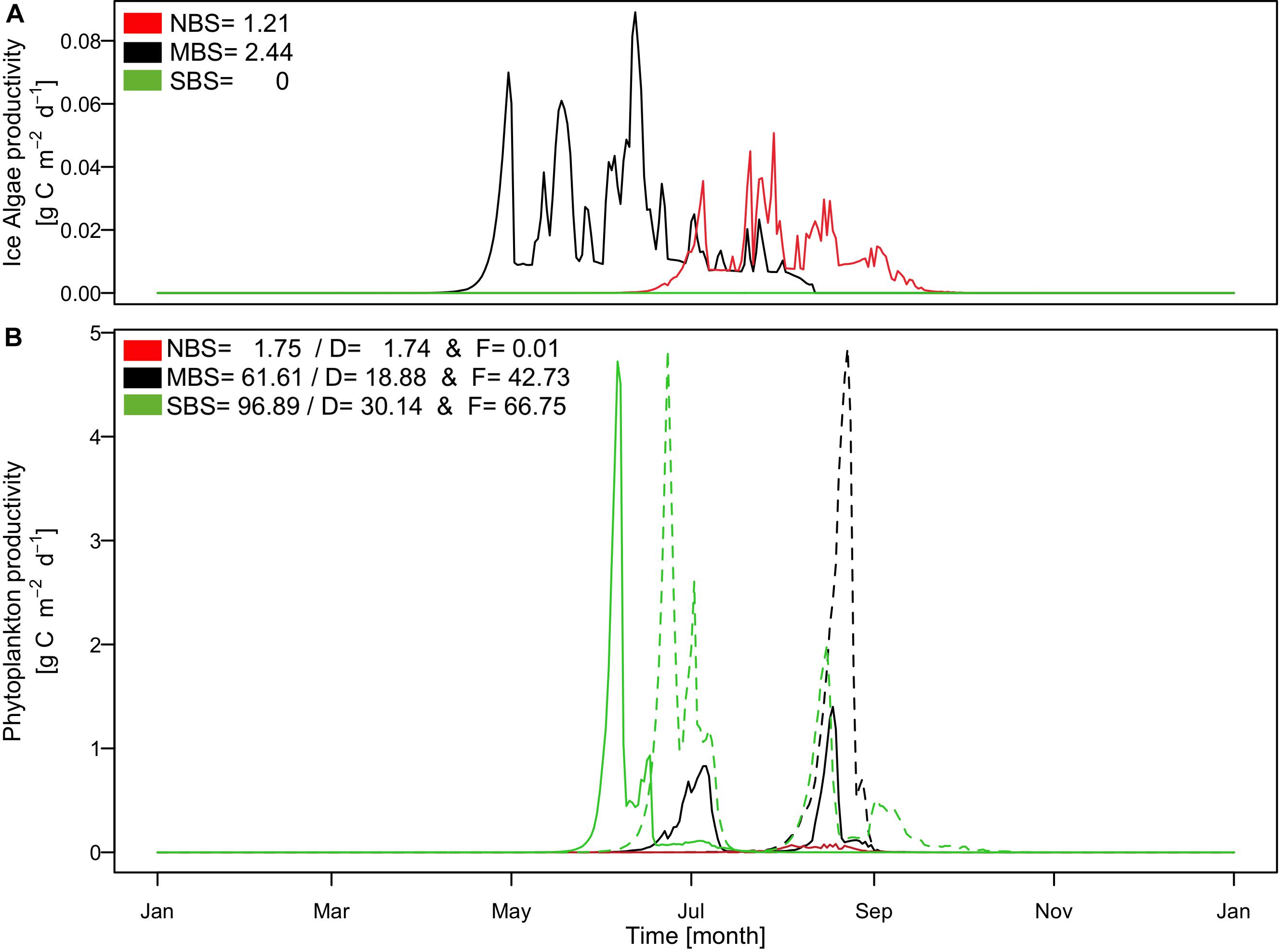
Figure 8. Simulated time series of (A) production rates of ice algae; (B) production rates of phytoplankton including diatoms (D: solid line) and flagellates (F: dashed line). Black color presents result for the central Barents Sea station over the 1997, red color for the north Barents Sea station over the 1997, and green color for the south Barents Sea station over the 1997. In the legend (A,B) are indicated the annual production in gC m^–2 for ice algae and phytoplankton including diatoms production (D) and flagellates production (F).

FIGURE 9

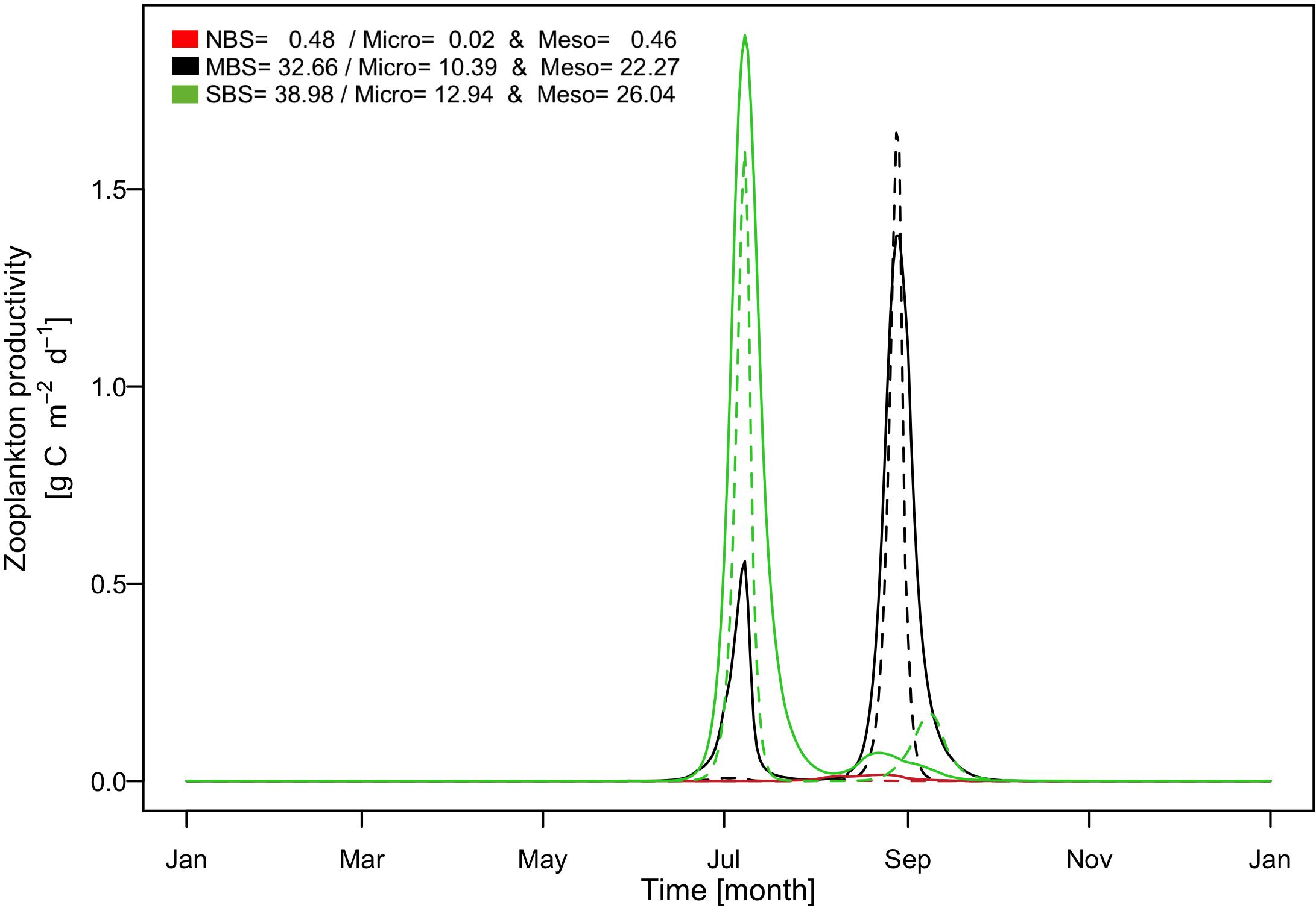
Figure 9. Simulated time series of production rates of zooplankton including mesozooplankton (solid line) and microzooplankton (dashed line). Black color presents result for the central Barents Sea station over the 1997, red color for the north Barents Sea station over the 1997, and green color for the south Barents Sea station over the 1997. In the legend are indicated the annual production in gC m^–2 for zooplankton including microzooplankton (Micro) and mesozooplankton (Meso).

For mesozooplankton and microzooplankton the seasonal dynamics followed closely phytoplankton blooms (Figure 9). Thereby, in the south zooplankton were mainly concentrated at the beginning of July following the diatoms and first flagellate blooms and slightly developed at the fall. In the north, only very little mesozooplankton developed in August following the diatom bloom. In the central area the seasonal dynamics were very different featuring two major zooplankton peaks in July and September, respectively. Contrary to the phytoplankton phenologies our results indicated that no phenological shift occurred in secondary production between the southern and the central Barents Sea location. The reason was that the zooplankton also feeds on ice algae allowing an increase in zooplankton biomass even before the pelagic diatom bloom starts and therefore promoting an early peak in zooplankton biomass.

Another interesting emergent result is that although primary production in the south was around 30% higher than in the central Barents Sea, the zooplankton annual total production was not significantly different between these two regions suggesting a more efficient trophic transfer from phytoplankton to zooplankton, again caused by the feeding process of zooplankton on ice algae.

Going from north to south in the Barents Sea may also be indicative of the Barents Sea ecosystem through time. Considering the expected sea ice retreat in the light of climate change during the next decades in the Barents Sea, we can expect a change toward a more southern ecosystem in terms of structure and functioning. This means an increase in primary production for the central Barents Sea and an increase of both primary and secondary productions for the northernmost regions. Previous modeling studies have already highlighted the potential increase of primary production in the Arctic and in the Barents Sea due to climate change and sea ice reduction and support our study results (Arrigo et al., 2008; Holt et al., 2016). Because the Arctic ecosystem structure has a relatively low complexity with few key players (Darnis et al., 2012), changes in the sea ice extent and ecosystem can greatly affect the whole Arctic food-web structure and functioning. As an example, according to the modeling study of Suprenand et al. (2018) important changes in zooplankton have already happened in the Beaufort Sea, and suggest greater changes in the marine ecosystem will occur in the next decades due to the sea ice decrease and temperature increase presently ongoing. Several species directly or indirectly depend on the ice algae, especially female Calanus for the eggs production as already discussed before.

Interannual Variability Pattern of Primary and Secondary Production

An additionally performed multi-year simulation experiment in the central Barents Sea highlights the interannual variability in this area (Sakshaug et al., 2009) with respect to magnitude and seasonality in primary and secondary production (Table 5). Within the simulated 7 year time period total annual primary production varied in the range of 34.33–95.92 gC m^–2 y^–1, with associated response in secondary production, which varies in the range of 13.61–49.76 gC m^–2 y^–1. Over these years the ice algae production represented always less than 10% of the total annual primary production also with strong interannual variation. The results indicated that years with long ice seasons, but thin ice thickness were the most productive for the ice algae (e.g., 1998). Our results did not demonstrate a clear and recurring seasonal pattern over the years due to the high variability of the ice cover dynamic. We can highlight the existence of a relationship between the length of the ice season and productivity of the ecosystem, which was already described by Rysgaard et al. (1999), showing a clear linear relationship between the annual pelagic primary production and length of productive open water period. Figure 10 shows clearly how the timing of the ice break-up drives the magnitude of the primary production. It becomes evident that the earlier in the season the ice breaks up, the higher the total annual primary production, which is consistent with findings by Arrigo and van Dijken (2015). This result also implies an increase of the total primary production in the next decade with the decrease of sea ice coverage and thickness and with a shorter period of ice coverage. This trend is already ongoing and observed in the Barents Sea and the other Arctic Seas (Frey et al., 2018) and is expected to be extended northward in future. Our results however suggested that the maximum productivity did not occur in an ice-free year, but rather during a year showing thin ice coverage and an early ice break-up, as it happens in 1995. This finding indicates that primary production in the Barents Sea may not necessarily increase under upcoming ice-free conditions but could even decrease especially in areas with seasonal sea ice dynamics. Additional numerical experiments in a 3D context will help to explore this pattern further with respect to regional scales. Previous modeling work from Holt et al. (2016) agreed with the heterogeneous effects of the climate change and ice retreat on the Barents Sea productivity and showed for instance that, in contrast to the northern and north-eastern Barents Sea, in the coastal southern Barents Sea production is expected to decrease.

TABLE 5

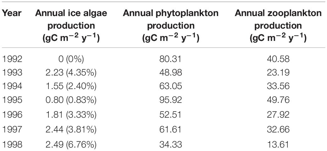
Table 5. Annual production of ice algae, phytoplankton (diatom + flagellate), and zooplankton (microzooplankton + mesozooplankton) for the central Barents Sea station over the 7 years simulated (1992–1998).

FIGURE 10

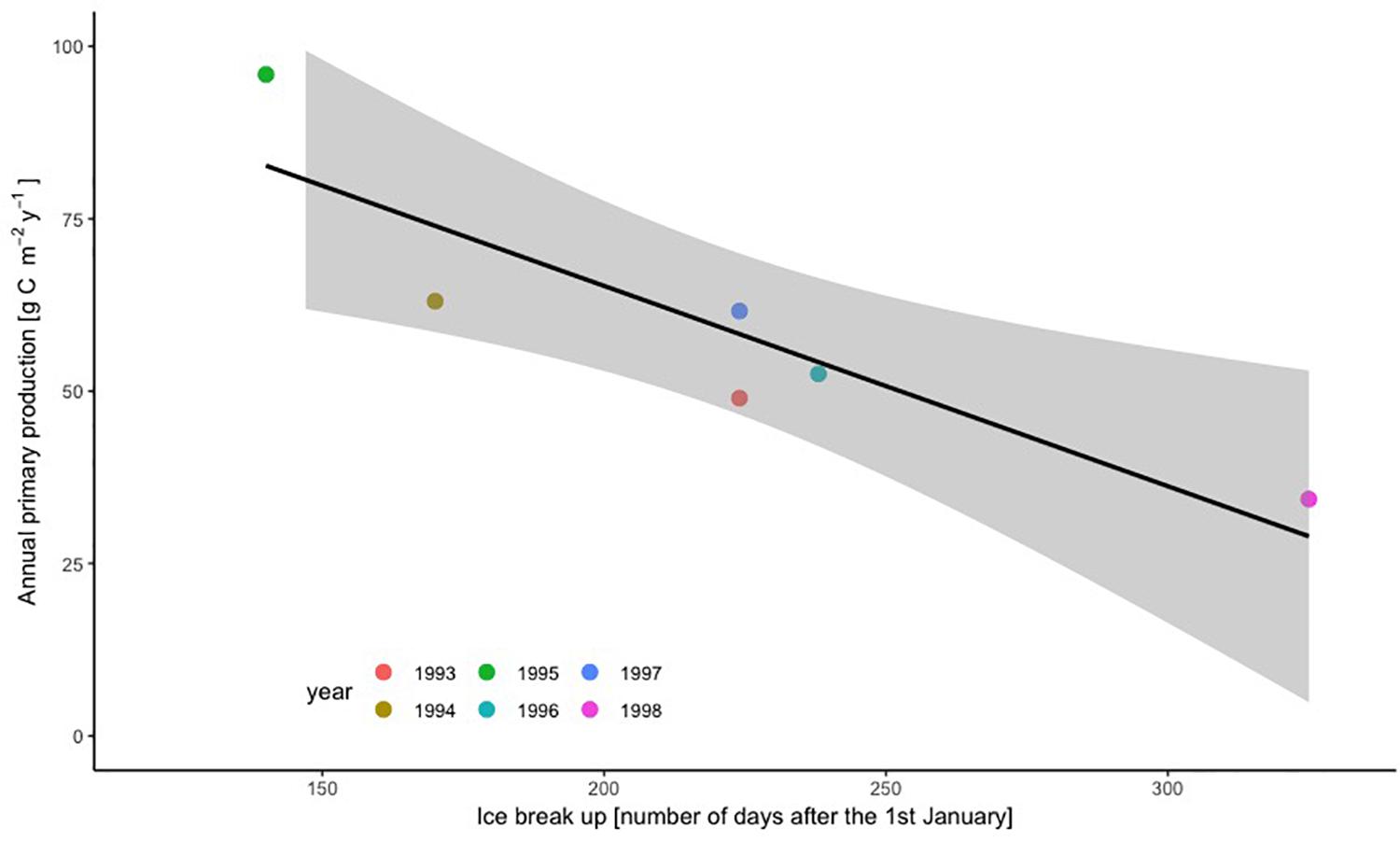
Figure 10. Relationship between annual primary production and ice break-up timing for the 7 years simulated at the central Barents Sea station. Values (p = 0.0159, R² adjusted = 0.75).

Conclusion

The overarching objective of our modeling approach was to understand the linkage between sympagic and pelagic ecosystem components by implementing a sympagic component to the biogeochemical model ECOSMO. We used the model in 1D at different locations in the Barents Sea ecosystem and analyzed spatial and interannual differences in ecosystem dynamics. The sympagic model component was based on previous developments (Lavoie et al., 2005; Tedesco and Vichi, 2014; Castellani et al., 2017; Vancoppenolle and Tedesco, 2017) and meant to improve the ECOSMO model performance in the Arctic ecosystem. In general, our results showed that the simulated seasonality of the sympagic components were realistic and in line with the current knowledge of the Barents Sea ecosystem. Compared to earlier model applications, our study specifically highlighted the strong interactions between the sympagic and the pelagic ecosystems. Most importantly, we could show that the ice algae play an important role for zooplankton phenology as it allows zooplankton biomass growth prior to the onset of the pelagic spring bloom. This process consequently determines the whole ecosystem structure as the zooplankton impacts the amplitude and the timing of the pelagic primary and secondary production. Additional relevant processes are the timing of the ice break-up and that ice algae production determine the phenologies of phytoplankton through seeding. Therefore, we propose that a fully coupled pelagic-sympagic ecosystem is a prerequisite to simulate the Arctic Ocean ecosystem and its changes correctly.

Exchange processes at the ice-ocean interface remain still poorly understood and our sensitivity analyses showed that the parametrization of these processes is a key component for our understanding of the Arctic ecosystem dynamics. With our approach we also found that the proportion of ice algae released and surviving in the pelagic system had an effect on the phytoplankton and zooplankton dynamics. Consequently, slight changes in the ice dynamic can disturb the whole structure of the present Arctic system and can modify phenologies not only of phytoplankton but also all the others species closely related of the ice algae, such as zooplankton (Werner, 1997; Søreide et al., 2010; Kohlbach et al., 2017a), fish (Kohlbach et al., 2017b; Steiner et al., 2019), or bird (Ramírez et al., 2017; Cusset et al., 2019). As an example, Polar cod (Boreogadus saida) is a central key species of the Arctic ecosystem and it is closely related to the ice algae especially during their larval development feeding on amphipods, which directly grazed on ice algae and sometimes directly feeding on ice algae itself (Gilbert et al., 1992; Kohlbach et al., 2017b). A decrease in the ice coverage will consequently affect the life cycle of Polar cod, by either creating a mismatch situation with the ice algae or changing the diet of larval Polar cod. We should expect changes in the Polar cod distribution in the next decades, with migration northward, and potentially an extension of the capelin population to replace the Polar cod as already suggested by Hop and Gjøsæter (2013) in the Barents Sea and Steiner et al. (2019) in the Western Canadian Arctic. Moreover, we can expect important change in the abundance and distribution of the predators feeding on both Polar cod and capelin. This example demonstrates, that further numerical experiments including higher trophic level of the marine ecosystem and coupling in a 3D framework will allow us to further explore these hypotheses.

Due to the harsh environmental conditions the Arctic remains a poorly sampled ecosystem leaving many uncertainties in the understanding of its ecosystem functioning. In the context of rapid climate changes, collaborative work becomes even more urgent to fill the knowledge gaps and improve our understanding of the Arctic system in order to establish sustainable management plan in the next decades.

Data Availability Statement

The raw data supporting the conclusions of this article will be made available by the authors, without undue reservation.

Author Contributions

DB performed and analyzed the biogeochemical model simulations. DB and UD wrote the main manuscript. All authors discussed the results and implications and participated in the manuscript improvement at all stages.

Funding

This work was jointly funded by the UK Research and Innovation Natural Environment Research Council (NERC) and the German Federal Ministry of Education and Research (BMBF).

Conflict of Interest

The authors declare that the research was conducted in the absence of any commercial or financial relationships that could be construed as a potential conflict of interest.

Acknowledgments

This work resulted from the MiMeMo projects (NE/R012571/1 and NE/R012679/1), part of the Changing Arctic Ocean program. We acknowledge particularly Richard Hofmeister for his valuable help on the model designing and programming process. We also acknowledge colleagues from the MiMeMo project, HZG institute and from the BEPSII (Biogeochemical Exchange Processes at the Sea-Ice Interfaces) for the useful discussions and comments. We are thankful for the insightful comments of the two reviewers and the editor.

References

Ambrose, W. G., von Quillfeldt, C., Clough, L. M., Tilney, P. V. R., and Tucker, T. (2005). The sub-ice algal community in the Chukchi sea: large- and small-scale patterns of abundance based on images from a remotely operated vehicle. Polar Biol. 28, 784–795. doi: 10.1007/s00300-005-0002-8

CrossRef Full Text | Google Scholar

Anisimov, O., and Fitzharris, B. (2001). “Polar Regions (Arctic and Antarctic). In Climate change 2001: Impacts, adaptation and vulnerability,” in Contribution of Working Group II to the Third Assesment Report of the Intergovernmental Panel on Climate Change, ed. K. S. White, (Cambridge: Cambridge University Press), 801–842.

Google Scholar

Arrigo, K. R. (2014). Sea Ice Ecosystems. Ann. Rev. Mar. Sci. 6, 439–467. doi: 10.1146/annurev-marine-010213-135103

PubMed Abstract | CrossRef Full Text | Google Scholar

Arrigo, K. R., Kremer, J. N., and Sullivan, C. W. (1993). A simulated Antarctic fast ice ecosystem. J. Geophys Res. 98, 6929–6946. doi: 10.1029/93JC00141

CrossRef Full Text | Google Scholar

Arrigo, K. R., and Sullivan, C. W. (1992). The influence of salinity and temperature covariation on the photophysiological characteristics of antarctic sea ice microalgae. J. Phycol. 28, 746–756. doi: 10.1111/j.0022-3646.1992.00746.x

CrossRef Full Text | Google Scholar

Arrigo, K. R., van Dijken, G., and Pabi, S. (2008). Impact of a shrinking Arctic ice cover on marine primary production. Geophys. Res. Lett. 35:L19603. doi: 10.1029/2008GL035028

CrossRef Full Text | Google Scholar

Arrigo, K. R., and van Dijken, G. L. (2015). Continued increases in arctic ocean primary production. Prog. Oceanogr 136, 60–70. doi: 10.1016/j.pocean.2015.05.002

CrossRef Full Text | Google Scholar

Årthun, M., Eldevik, T., Smedsrud, L. H., and Skagseth, Ø, and Ingvaldsen, R. B. (2012). Quantifying the influence of atlantic heat on barents sea ice variability and retreat. J. Clim. 25, 4736–4743. doi: 10.1175/JCLI-D-11-00466.1

CrossRef Full Text | Google Scholar

Belém, A. L. (2002). Modeling Physical and Biological Processes in Antarctic Sea Ice. Dissertation thesis. Bremen: Universitat Bremen.

Google Scholar

Bennett, J. R., Shaw, J. D., Terauds, A., Smol, J. P., Aerts, R., Bergstrom, D., et al. (2015). Polar lessons learned: long-term management based on shared threats in Arctic and Antarctic environments. Front. Ecol. Environ. 13:316–324. doi: 10.1890/140315

CrossRef Full Text | Google Scholar

Bleck, R. (2002). An oceanic general circulation model framed in hybrid isopycnic-Cartesian coordinates. Ocean Model. 4, 55–88. doi: 10.1016/S1463-5003(01)00012-9

CrossRef Full Text | Google Scholar

Boetius, A., Albrecht, S., Bakker, K., Bienhold, C., Felden, J., and Fernández-Méndez, M. (2013). Export of algal biomass from the melting arctic sea ice. Science 339, 1430. doi: 10.1126/science.1231346

PubMed Abstract | CrossRef Full Text | Google Scholar

Bouchard, C., Geoffroy, M., LeBlanc, M., and Fortier, L. (2018). Larval and adult fish assemblages along the Northwest Passage: the shallow Kitikmeot and the ice-covered Parry Channel as potential barriers to dispersal. Arct. Sci. 4, 781–793. doi: 10.1139/as-2018-0003

CrossRef Full Text | Google Scholar

Boyer, T. P., Antonov, J. I., Baranova, O. K., Coleman, C., Garcia, H. E., and Grodsky, A. (2013). “World Ocean Database 2013,” in NOAA Atlas NESDIS 72, eds S. Levitus and A. Mishonov, (Silver Spring, MD: National Oceanographic Data Center), 209. doi: 10.7289/V5NZ85MT

CrossRef Full Text | Google Scholar

Bruggeman, J., and Bolding, K. (2014). A general framework for aquatic biogeochemical models. Environ. Model. Softw. 61, 249–265. doi: 10.1016/j.envsoft.2014.04.002

CrossRef Full Text | Google Scholar

Burchard, H., Bolding, K., and Villarreal, M. R. (1999). GOTM, A General Ocean Turbulence Model. Theory, Implementation And Test Cases. Greece: Space Applications Institute,.

Google Scholar

Castellani, G., Losch, M., Lange, B. A., and Flores, H. (2017). Modeling Arctic sea-ice algae: physical drivers of spatial distribution and algae phenology. J. Geophys. Res. Ocean. 122, 7466–7487. doi: 10.1002/2017JC012828

CrossRef Full Text | Google Scholar

Clark, G. F., Stark, J. S., Palmer, A. S., Riddle, M. J., and Johnston, E. L. (2017). The roles of sea-ice, light and sedimentation in structuring shallow antarctic benthic communities. PLoS One 12:e0168391. doi: 10.1371/journal.pone.0168391

PubMed Abstract | CrossRef Full Text | Google Scholar

Clasby, R. C., Horner, R., and Alexander, V. (1973). An in situ method for measuring primary productivity of arctic sea ice algae. J. Fish Res. Board Can. 30, 835–838. doi: 10.1139/f73-139

CrossRef Full Text | Google Scholar

Cottier, F., Steele, M., and Nilsen, F. (2017). Sea ice and Arctic Ocean Oceanography. Hoboken, NJ: John Wiley &Sons, 197–215. doi: 10.1002/9781118778371.ch7

CrossRef Full Text | Google Scholar

Cusset, F., Fort, J., Mallory, M., Braune, B., Massicotte, P., and Massé, G. (2019). Arctic seabirds and shrinking sea ice: egg analyses reveal the importance of ice-derived resources. Sci. Rep. 9:15405. doi: 10.1038/s41598-019-51788-4

PubMed Abstract | CrossRef Full Text | Google Scholar

Daewel, U., and Schrum, C. (2013). Simulating long-term dynamics of the coupled North Sea and Baltic Sea ecosystem with ECOSMO II: model description and validation. J. Mar. Syst. 119, 30–49. doi: 10.1016/j.jmarsys.2013.03.008

CrossRef Full Text | Google Scholar

Daewel, U., Schrum, C., and Macdonald, J. (2019). Towards End-2-End modelling in a consistent NPZD-F modelling framework (ECOSMOE2E_vs1.0): application to the North Sea and Baltic Sea. Geosci. Model Dev. Discuss. 2019, 1–40. doi: 10.5194/gmd-2018-239

CrossRef Full Text | Google Scholar

Dalpadado, P., Arrigo, K. R., Hjøllo, S. S., Rey, F., Ingvaldsen, R. B., Sperfeld, E., et al. (2014). Productivity in the barents sea–response to recent climate variability. PLoS One 9:e095273. doi: 10.1371/journal.pone.0095273

PubMed Abstract | CrossRef Full Text | Google Scholar

Darnis, G., Robert, D., Pomerleau, C., Link, H., Archambault, P., Nelson, R. J., et al. (2012). Current state and trends in Canadian Arctic marine ecosystems: II. Heterotrophic food web, pelagic-benthic coupling, and biodiversity. Clim. Change 115, 179–205. doi: 10.1007/s10584-012-0483-8

CrossRef Full Text | Google Scholar

Deal, C., Jin, M., Elliott, S., Hunke, E., Maltrud, M., and Jeffery, N. (2011). Large-scale modeling of primary production and ice algal biomass within arctic sea ice in 1992. J. Geophys, Res. Ocean 116, 148–227. doi: 10.1029/2010JC006409

Google Scholar

Dezutter, T., Lalande, C., Dufresne, C., Darnis, G., and Fortier, L. (2019). Mismatch between microalgae and herbivorous copepods due to the record sea ice minimum extent of 2012 and the late sea ice break-up of 2013 in the Beaufort Sea. Prog. Oceanogr. 173, 66–77. doi: 10.1016/j.pocean.2019.02.008

CrossRef Full Text | Google Scholar

Diebold, F. X., and Rudebusch, G. D. (2019). Probability Assessments Of An Ice-Free Arctic: Comparing Statistical And Climate Model Projections. PIER Working Paper No. 20-001, University of Pennsylvania, Philadelphia, PA. doi: 10.2139/ssrn.3513025

PubMed Abstract | CrossRef Full Text | Google Scholar

Duarte, P., Assmy, P., Hop, H., Spreen, G., Gerland, S., and Hudson, S. R. (2015). The importance of vertical resolution in sea ice algae production models. Mar. J. Syst. 145, 69–90. doi: 10.1016/j.jmarsys.2014.12.004

CrossRef Full Text | Google Scholar

Durbin, E. G., and Casas, M. C. (2014). Early reproduction by Calanus glacialis in the Northern Bering Sea: the role of ice algae as revealed by molecular analysis. J. Plankton Res. 36, 523–541. doi: 10.1093/plankt/fbt121

PubMed Abstract | CrossRef Full Text | Google Scholar

Eppley, R. W. (1972). Temperature and phytoplankton growth in the sea. Fish. Bull. 70, 1063–1085.

Google Scholar

Fernández-Méndez, M., Olsen, L. M., Kauko, H. M., Meyer, A., Rösel, A., and Merkouriadi, L. (2018). Algal hot spots in a changing Arctic Ocean: sea-ice ridges and the snow-ice interface. Front. Mar. Sci. 5:75. doi: 10.3389/fmars.2018.00075

CrossRef Full Text | Google Scholar

Frey, K. E., Comiso, J. C., Cooper, L. W., Grebmeier, J. M., and Stock, L. V. (2018). “Arctic ocean primary productivity: The response of marine algae to climate warming and sea ice decline,” in Arctic Report Card Update 2018, eds E. Osborne, J. Richter-Menge, and M. Jeffries, (Washingdon, DC: NOAA).

Google Scholar

Galindo, V., Gosselin, M., Lavaud, J., Mundy, C. J., Else, B., Ehn, J., et al. (2017). Pigment composition and photoprotection of Arctic sea ice algae during spring. Mar. Ecol. Prog. Ser. 585, 49–69. doi: 10.3354/meps12398

CrossRef Full Text | Google Scholar

Galindo, V., Levasseur, M., Mundy, C. J., Tremblay, J.-E., Scarratt, M., Gratton, Y., et al. (2014). Biological and physical processes influencing sea ice, under-ice algae, and dimethylsulfoniopropionate during spring in the Canadian Arctic Archipelago. J. Geophys. Res. Ocean. 119, 3746–3766. doi: 10.1002/2013JC009497

CrossRef Full Text | Google Scholar

Gilbert, M., Fortier, L., Ponton, D., and Drolet, R. (1992). Feeding ecology of marine fish larvae across the Great Whale River plume in seasonally ice-covered southeastern Hudson Bay. Mar. Ecol. Prog. Ser. Oldend. 84, 19–30.

Google Scholar

Gosselin, M., Levasseur, M., Wheeler, P. A., Horner, R. A., and Booth, B. C. (1997). New measurements of phytoplankton and ice algal production in the Arctic Ocean. Deep. Res. Part II Top. Stud. Oceanogr. 44, 1623–1644. doi: 10.1016/S0967-0645(97)00054-4

CrossRef Full Text | Google Scholar

Gradinger, R., Friedrich, C., and Spindler, M. (1999). Abundance, biomass and composition of the sea ice biota of the Greenland Sea pack ice. Deep Sea Res. Part II Top. Stud. Oceanogr. 46, 1457–1472. doi: 10.1016/S0967-0645(99)00030-2

CrossRef Full Text | Google Scholar

Haecky, P., Jonsson, S., and Andersson, A. (1998). Influence of sea ice on the composition of the spring phytoplankton bloom in the northern Baltic Sea. Polar Biol. 20, 1–8. doi: 10.1007/s003000050270

CrossRef Full Text | Google Scholar

Hegseth, E. N. (1992). Sub-ice algal assemblages of the Barents Sea: species composition, chemical composition, and growth rates. Polar Biol. 12, 485–496. doi: 10.1007/BF00238187

CrossRef Full Text | Google Scholar

Hegseth, E. N. (1998). Primary production of the northern Barents Sea. Polar Res. 17, 113–123. doi: 10.1111/j.1751-8369.1998.tb00266.x

CrossRef Full Text | Google Scholar

Hirche, H.-J., and Kosobokova, K. (2003). Early reproduction and development of dominant calanoid copepods in the sea ice zone of the Barents Sea—need for a change of paradigms? Mar. Biol. 143, 769–781. doi: 10.1007/s00227-003-1122-8

CrossRef Full Text | Google Scholar

Holt, J., Schrum, C., Cannaby, H., Daewel, U., Allen, I., Artioli, Y., et al. (2016). Potential impacts of climate change on the primary production of regional seas: a comparative analysis of five European seas. Prog. Oceanogr. 140, 91–115. doi: 10.1016/j.pocean.2015.11.004

CrossRef Full Text | Google Scholar

Hop, H., and Gjøsæter, H. (2013). Polar cod (Boreogadus saida) and capelin (Mallotus villosus) as key species in marine food webs of the Arctic and the Barents Sea. Mar. Biol. Res. 9, 878–894. doi: 10.1080/17451000.2013.775458

CrossRef Full Text | Google Scholar

Horner, R., and Alexander, V. (1972). Algal populations in Arctic sea ice: an investigation of heterotrophy. Limnol. Oceanogr. 17, 454–458. doi: 10.4319/lo.1972.17.3.0454

CrossRef Full Text | Google Scholar

Jin, M., Deal, C., Wang, J., Alexander, V., Gradinger, R., and Saitoh, S.-I. (2007). Ice-associated phytoplankton blooms in the southeastern Bering Sea. Geophys. Res. Lett. 34, 94–8276. doi: 10.1029/2006GL028849

CrossRef Full Text | Google Scholar

Jin, M., Deal, C. J., Wang, J. K., Shin, H., Tanaka, N., Whitledge, T. E., et al. (2006). Controls of the landfast ice–ocean ecosystem offshore Barrow, Alaska. Ann. Glaciol. 44, 63–72. doi: 10.3189/172756406781811709

CrossRef Full Text | Google Scholar

Juul-Pedersen, T., Michel, C., Gosselin, M., and Seuthe, L. (2008). Seasonal changes in the sinking export of particulate material under first-year sea ice on the Mackenzie Shelf (western Canadian Arctic). Mar. Ecol. Prog. Ser. 353, 13–25. doi: 10.3354/meps07165

CrossRef Full Text | Google Scholar

Kanamitsu, M., Ebisuzaki, W., Woollen, J., Yang, S.-K., Hnilo, J. J., Fiorino, M., et al. (2002). NCEP–DOE AMIP-II Reanalysis (R-2). Bull. Am. Meteorol. Soc. 83, 1631–1644. doi: 10.1175/BAMS-83-11-1631

CrossRef Full Text | Google Scholar

Kauko, H. M., Olsen, L. M., Duarte, P., Peeken, I., Granskog, M. A., Johnsen, G., et al. (2018). Algal colonization of young arctic sea ice in spring. Front. Mar. Sci. 5:199. doi: 10.3389/fmars.2018.00199

CrossRef Full Text | Google Scholar

Kimura, N., and Wakatsuchi, M. (2001). Mechanisms for the variation of sea ice extent in the Northern Hemisphere. Geophys, J., Res. Ocean. 106, 31319–31331. doi: 10.1029/2000jc000739

CrossRef Full Text | Google Scholar

Koenigk, T., Mikolajewicz, U., Jungclaus, J. H., and Kroll, A. (2009). Sea ice in the Barents Sea: seasonal to interannual variability and climate feedbacks in a global coupled model. Clim. Dyn. 32, 1119–1138. doi: 10.1007/s00382-008-0450-2

CrossRef Full Text | Google Scholar

Kohlbach, D., Ferguson, S. H., Brown, T. A., and Michel, C. (2019). Landfast sea ice-benthic coupling during spring and potential impacts of system changes on food web dynamics in Eclipse Sound, Canadian Arctic. Mar. Ecol. Prog. Ser. 627, 33–48.

Google Scholar

Kohlbach, D., Graeve, M., Lange, B. A., David, C., Peeken, I., and Flores, H. (2016). The importance of ice algae-produced carbon in the central Arctic Ocean ecosystem: food web relationships revealed by lipid and stable isotope analyses. Limnol. Oceanogr. 61, 2027–2044. doi: 10.1002/lno.10351

CrossRef Full Text | Google Scholar

Kohlbach, D., Lange, B. A., Schaafsma, F. L., David, C., Vortkamp, M., Graeve, M., et al. (2017a). Ice algae-produced carbon is critical for overwintering of antarctic krill Euphausia superba. Front. Mar. Sci. 4:310. doi: 10.3389/fmars.2017.00310

CrossRef Full Text | Google Scholar

Kohlbach, D., Schaafsma, F. L., Graeve, M., Lebreton, B., Lange, B. A., David, C., et al. (2017b). Strong linkage of polar cod (Boreogadus saida) to sea ice algae-produced carbon: evidence from stomach content, fatty acid and stable isotope analyses. Prog. Oceanogr. 152, 62–74. doi: 10.1016/j.pocean.2017.02.003

CrossRef Full Text | Google Scholar

Kwok, R. (2009). Outflow of Arctic Ocean sea ice into the Greenland and Barent Seas: 1979-2007. Clim. J. 22, 2438–2457. doi: 10.1175/2008JCLI2819.1

CrossRef Full Text | Google Scholar

Lavoie, D., Denman, K., and Michel, C. (2005). Modeling ice algal growth and decline in a seasonally ice-covered region of the Arctic (Resolute Passage, Canadian Archipelago). J. Geophys. Res. Ocean 110:C11009. doi: 10.1029/2005JC002922

CrossRef Full Text | Google Scholar

Legendre, L., Ackley, S. F., Dieckmann, G. S., Gulliksen, B., Horner, R., and Hoshiai, T. (1992). Ecology of sea ice biota. Polar Biol. 12, 429–444. doi: 10.1007/BF00243114

CrossRef Full Text | Google Scholar

Leu, E., Søreide, J. E., Hessen, D. O., Falk-Petersen, S., and Berge, J. (2011). Consequences of changing sea-ice cover for primary and secondary producers in the European Arctic shelf seas: timing, quantity, and quality. Prog. Oceanogr. 90, 18–32. doi: 10.1016/j.pocean.2011.02.004

CrossRef Full Text | Google Scholar

Lindsay, R., and Schweiger, A. (2015). Arctic sea ice thickness loss determined using subsurface, aircraft, and satellite observations. Cryosphere 9, 269–283. doi: 10.5194/tc-9-269-2015

CrossRef Full Text | Google Scholar

Lizotte, M. P. (2001). The contributions of sea ice algae to antarctic marine primary production1. Am. Zool. 41, 57–73. doi: 10.1093/icb/41.1.57

CrossRef Full Text | Google Scholar

Luchetta, A., Lipizer, M., and Socal, G. (2000). Temporal evolution of primary production in the central Barents Sea. J. Mar. Syst. 27, 177–193. doi: 10.1016/S0924-7963(00)00066-X

CrossRef Full Text | Google Scholar

Mangoni, O., Saggiomo, M., Modigh, M., Catalano, G., Zingone, A., and Saggiomo, V. (2009). The role of platelet ice microalgae in seeding phytoplankton blooms in Terra Nova Bay (Ross Sea. Antarctica): a mesocosm experiment. Polar Biol. 32, 311–323. doi: 10.1007/s00300-008-0507-z

CrossRef Full Text | Google Scholar

McMahon, K. W., Ambrose, W. G. Jr, Johnson, B. J., Sun, M.-Y., Lopez, G. R., Clough, L. M., et al. (2006). Benthic community response to ice algae and phytoplankton in Ny Alesund. Svalbard. Mar. Ecol. Prog. Ser. 310, 1–14. doi: 10.3354/meps310001

CrossRef Full Text | Google Scholar

McMinn, A., and Hegseth, E. N. (2007). Sea ice primary productivity in the northern Barents Sea, spring 2004. Polar Biol. 30, 289–294. doi: 10.1007/s00300-006-0182-x

CrossRef Full Text | Google Scholar

McPhee, M. G. (2017). The Sea Ice–Ocean Boundary Layer. Hoboken, NJ: John Wiley & Sons, Ltd, 138–159. doi: 10.1002/9781118778371.ch5

CrossRef Full Text | Google Scholar

Meier, W. N. (2017). Losing Arctic Sea Ice: Observations of the Recent Decline and the Long-Term Context. Hoboken, NJ: John Wiley & Sons, Ltd, 290–303. doi: 10.1002/9781118778371.ch11

CrossRef Full Text | Google Scholar

Michel, C., Legendre, L., Ingram, R. G., Gosselin, M., and Levasseur, M. (1996). Carbon budget of sea-ice algae in spring: evidence of a significant transfer to zooplankton grazers. J. Geophys. Res. Ocean. 101, 18345–18360. doi: 10.1029/96JC00045

CrossRef Full Text | Google Scholar

Michel, C., Nielsen, T. G., Nozais, C., and Gosselin, M. (2002). Significance of sedimentation and grazing by ice micro-and meiofauna for carbon cycling in annual sea ice (northern Baffin Bay). Aquat. Microb. Ecol. 30, 57–68. doi: 10.3354/ame030057

CrossRef Full Text | Google Scholar

Monod, J. (1949). The growth of bacterial cultures. Annu. Rev. Microbiol. 3, 371–394. doi: 10.1146/annurev.mi.03.100149.002103

CrossRef Full Text | Google Scholar

Mortenson, E., Hayashida, H., Steiner, N., Monahan, A., Blais, M., Gale, M. A., et al. (2017). A model-based analysis of physical and biological controls on ice algal and pelagic primary production in Resolute Passage. Elem. Sci. Anth. 5:39. doi: 10.1525/elementa.229

PubMed Abstract | CrossRef Full Text | Google Scholar

Mundy, C., Gosselin, M., Gratton, Y., Brown, K., Galindo, V., Campbell, K., et al. (2014). Role of environmental factors on phytoplankton bloom initiation under landfast sea ice in Resolute Passage. Canada. Mar. Ecol. Prog. Ser. 497, 39–49. doi: 10.3354/meps10587

CrossRef Full Text | Google Scholar

Niemi, A., Michel, C., Hille, K., and Poulin, M. (2011). Protist assemblages in winter sea ice: setting the stage for the spring ice algal bloom. Polar Biol. 34, 1803–1817. doi: 10.1007/s00300-011-1059-1

CrossRef Full Text | Google Scholar

Olsen, L. M., Laney, S. R., Duarte, P., Kauko, H. M., Fernández-Méndez, M., Mundy, C. J., et al. (2017). The seeding of ice algal blooms in Arctic pack ice: the multiyear ice seed repository hypothesis. J. Geophys. Res. Biogeosci. 122, 1529–1548. doi: 10.1002/2016JG003668

CrossRef Full Text | Google Scholar

Onarheim, I. H., and Årthun, M. (2017). Toward an ice-free Barents Sea. Geophys. Res. Lett. 44, 8387–8395. doi: 10.1002/2017GL074304

CrossRef Full Text | Google Scholar

Oziel, L., Massicotte, P., Randelhoff, A., Ferland, J., Vladoiu, A., and Lacour, L. (2019). Environmental factors influencing the seasonal dynamics of spring algal blooms in and beneath sea ice in western Baffin Bay. Elem. Sci. Anthr. Univ. Calif. Press 7:34. doi: 10.1525/elementa.372

PubMed Abstract | CrossRef Full Text | Google Scholar

Peng, G., and Meier, W. N. (2018). Temporal and regional variability of Arctic sea-ice coverage from satellite data. Ann. Glaciol. 59, 191–200. doi: 10.1017/aog.2017.32

CrossRef Full Text | Google Scholar

Pourchez, A. (2018). Impact de la Diapause sur la Dynamique de Communautés Planctonique dans un Écosystème Arctique Numérique. Master’s thesis. Quebec, QL: Universté Laval.

Google Scholar

Ramírez, F., Tarroux, A., Hovinen, J., Navarro, J., Afán, I., Forero, M. G., et al. (2017). Sea ice phenology and primary productivity pulses shape breeding success in Arctic seabirds. Sci. Rep. 7:4500. doi: 10.1038/s41598-017-04775-6

PubMed Abstract | CrossRef Full Text | Google Scholar

Ratkova, T. N., and Wassmann, P. (2005). Sea ice algae in the White and Barents seas: composition and origin. Polar Res. 24, 95–110. doi: 10.3402/polar.v24i1.6256

CrossRef Full Text | Google Scholar

Reigstad, M., Wassmann, P., Wexels Riser, C., Øygarden, S., and Rey, F. (2002). Variations in hydrography, nutrients and chlorophyll a in the marginal ice-zone and the central Barents Sea. Mar, J., Syst. 38, 9–29. doi: 10.1016/S0924-7963(02)00167-7

CrossRef Full Text | Google Scholar

Riebesell, U., Schloss, I., and Smetacek, V. (1991). Aggregation of algae released from melting sea ice: implications for seeding and sedimentation. Polar Biol. 11, 239–248. doi: 10.1007/BF00238457

CrossRef Full Text | Google Scholar

Rózańska, M., Gosselin, M., Poulin, M., Jm, W., and Michel, C. (2009). Influence of environmental factors on the development of bottom ice protist communities during the winter–spring transition. Mar. Ecol. Prog. Ser. 386, 43–59. doi: 10.3354/meps08092

CrossRef Full Text | Google Scholar

Runge, J. A., and Ingram, R. G. (1988). Underice grazing by planktonic, calanoid copepods in relation to a bloom of ice microalgae in southeastern Hudson Bay. Limnol. Oceanogr. 33, 280–286. doi: 10.4319/lo.1988.33.2.0280

CrossRef Full Text | Google Scholar

Runge, J. A., and Ingram, R. G. (1991). Under-ice feeding and diel migration by the planktonic copepods Calanus glacialis and Pseudocalanus minutus in relation to the ice algal production cycle in southeastern Hudson Bay. Canada. Mar. Biol. 108, 217–225. doi: 10.1007/BF01344336

CrossRef Full Text | Google Scholar

Rysgaard, S., Nielsen, T. G., and Hansen, B. W. (1999). Seasonal variation in nutrients, pelagic primary production and grazing in a high-Arctic coastal marine ecosystem. Young Sound, Northeast Greenland. Mar. Ecol. Prog. Ser. 179, 13–25. doi: 10.3354/meps179013

CrossRef Full Text | Google Scholar

Sakshaug, E. (1997). Biomass and productivity distributions and their variability in the Barents Sea. ICES Mar. J. Sci. 54, 341–350. doi: 10.1006/jmsc.1996.0170

CrossRef Full Text | Google Scholar

Sakshaug, E., Johnsen, G. H., and Kovacs, K. M. (2009). Ecosystem Barents Sea, Tapir. Cambridge, MA: Academic Press.

Google Scholar

Samuelsen, A., Hansen, C., and Wehde, H. (2015). Tuning and assessment of the HYCOM-NORWECOM V2.1 biogeochemical modeling system for the North Atlantic and Arctic oceans. Geosci. Model Dev. 8, 2187–2202. doi: 10.5194/gmd-8-2187-2015

CrossRef Full Text | Google Scholar

Sarthou, G., Timmermans, K. R., Blain, S., and Tréguer, P. (2005). Growth physiology and fate of diatoms in the ocean: a review. J. Sea Res. 53, 25–42. doi: 10.1016/j.seares.2004.01.007

CrossRef Full Text | Google Scholar

Schober, M., Duvenaud, D. K., and Hennig, P. (2014). Probabilistic ODE solvers with Runge-Kutta means. Adv. Neural Inf. Process. Syst. 2014, 739–747.

Google Scholar

Schollmeier, T., Oliveira, A. C. M., Wooller, M. J., and Iken, K. (2018). Tracing sea ice algae into various benthic feeding types on the Chukchi Sea shelf. Polar Biol. 41, 207–224. doi: 10.1007/s00300-017-2182-4

CrossRef Full Text | Google Scholar

Schrum, C., Alekseeva, I., and St John, M. (2006). Development of a coupled physical–biological ecosystem model ECOSMO: part I: model description and validation for the North Sea. J. Mar. Syst. 61, 79–99. doi: 10.1016/j.jmarsys.2006.01.005

CrossRef Full Text | Google Scholar

Selz, V., Saenz, B. T., van Dijken, G. L., and Arrigo, K. R. (2018). Drivers of Ice Algal Bloom Variability between 1980 and 2015 in the Chukchi Sea. J. Geophys. Res. Ocean 123, 7037-7052. doi: 10.1029/2018JC014123

CrossRef Full Text | Google Scholar

Sibert, V., Zakardjian, B., Saucier, F., Gosselin, M., Starr, M., and Senneville, S. (2010). Spatial and temporal variability of ice algal production in a 3D ice – ocean model of the Hudson Bay, Hudson Strait and Foxe Basin system Spatial and temporal variability of ice algal production in a 3D ice – ocean model of the Hudson Bay, Hudson Strait. Polar Res. 29, 353–378. doi: 10.3402/polar.v29i3.6084

CrossRef Full Text | Google Scholar

Skagseth, Ø, Eldevik, T., Årthun, M., Asbjørnsen, H., Lien, V. S., and Smedsrud, L. H. (2020). Reduced efficiency of the Barents Sea cooling machine. Nat. Clim. Change 10, 661–666. doi: 10.1038/s41558-020-0772-6

CrossRef Full Text | Google Scholar

Slagstad, D., Wassmann, P. F. J., and Ellingsen, I. (2015). Physical constrains and productivity in the future Arctic Ocean. Front. Mar. Sci. 2:85. doi: 10.3389/fmars.2015.00085

CrossRef Full Text | Google Scholar

Søreide, J. E., Carroll, M. L., Hop, H., Ambrose, W. G. Jr., Hegseth, E. N., and Falk-Petersen, S. (2013). Sympagic-pelagic-benthic coupling in Arctic and Atlantic waters around Svalbard revealed by stable isotopic and fatty acid tracers. Mar. Biol. Res. 9, 831–850. doi: 10.1080/17451000.2013.775457

CrossRef Full Text | Google Scholar

Søreide, J. E., Hop, H., Carroll, M. L., Falk-Petersen, S., and Hegseth, E. N. (2006). Seasonal food web structures and sympagic–pelagic coupling in the European Arctic revealed by stable isotopes and a two-source food web model. Prog. Oceanogr. 71, 59–87. doi: 10.1016/j.pocean.2006.06.001

CrossRef Full Text | Google Scholar

Søreide, J. E., Leu, E., Berge, J., Graeve, M., and Falk-Petersen, S. (2010). Timing of blooms, algal food quality and Calanus glacialis reproduction and growth in a changing Arctic. Glob. Chang Biol. 16, 3154–3163. doi: 10.1111/j.1365-2486.2010.02175.x

CrossRef Full Text | Google Scholar

Steiner, N., Deal, C., Lannuzel, D., Diane, L., François, M., and Lisa, A. (2016). What sea-ice biogeochemical modellers need from observers. Elem. Sci. Anth. 4:000084. doi: 10.12952/journal.elementa.000084

CrossRef Full Text | Google Scholar

Steiner, N. S., Cheung, W. W. L., Cisneros-Montemayor, A. M., Drost, H., Hayashida, H., Hoover, C., et al. (2019). Impacts of the changing ocean-sea ice system on the key forage fish arctic cod (Boreogadus Saida) and subsistence fisheries in the western canadian arctic—evaluating linked climate. ecosystem and economic (CEE) Models. Front. Mar. Sci. 6:179. doi: 10.3389/fmars.2019.00179

CrossRef Full Text | Google Scholar

Stretch, J. J., Hamner, P. P., Hamner, W. M., Michel, W. C., Cook, J., and Sullivan, C. W. (1988). Foraging behavior of Antarctic krill Euphausia superba on sea ice microalgae. Mar. Ecol. Prog. Ser 44, 131–139.

Google Scholar

Stroeve, J., and Notz, D. (2018). Changing state of Arctic sea ice across all seasons. Environ. Res. Lett. 13:103001.

Google Scholar

Stroeve, J. C., Serreze, M. C., Holland, M. M., Kay, J. E., Malanik, J., and Barrett, A. P. (2012). The Arctic’s rapidly shrinking sea ice cover: a research synthesis. Clim. Change 110, 1005–1027. doi: 10.1007/s10584-011-0101-1

CrossRef Full Text | Google Scholar

Sun, M.-Y., Carroll, M. L., Ambrose, W. G., Clough, L. M., Zou, L., and Lopez, G. R. (2007). Rapid consumption of phytoplankton and ice algae by Arctic soft-sediment benthic communities: evidence using natural and 13C-labeled food materials. J. Mar, Res. 65, 561–588. doi: 10.1357/002224007782689094

CrossRef Full Text | Google Scholar

Sun, M.-Y., Clough, L. M., Carroll, M. L., Dai, J., Ambrose, W. G., and Lopez, G. R. (2009). Different responses of two common Arctic macrobenthic species (Macoma balthica and Monoporeia affinis) to phytoplankton and ice algae: will climate change impacts be species specific? Exp, J., Mar. Bio. Ecol. 376, 110–121. doi: 10.1016/j.jembe.2009.06.018

CrossRef Full Text | Google Scholar

Sundfjord, A., Fer, I., Kasajima, Y., and Svendsen, H. (2007). Observations of turbulent mixing and hydrography in the marginal ice zone of the Barents Sea. Geophys, J., Res. Ocean 112:C05008. doi: 10.1029/2006JC003524

CrossRef Full Text | Google Scholar

Suprenand, P. M., Ainsworth, C. H., and Hoover, C. (2018). Ecosystem model of the entire beaufort sea marine ecosystem: a temporal tool for assessing food-web structure and marine animal populations from 1970 to 2014. Marine Science Faculty Publications 261.

Google Scholar

Syvertsen, E. E. (1991). Ice algae in the Barents Sea: types of assemblages, origin, fate and role in the ice-edge phytoplankton bloom. Polar Res. 10, 277–288. doi: 10.1111/j.1751-8369.1991.tb00653.x

CrossRef Full Text | Google Scholar

Szymanski, A., and Gradinger, R. (2016). The diversity, abundance and fate of ice algae and phytoplankton in the Bering Sea. Polar Biol. 39, 309–325. doi: 10.1007/s00300-015-1783-z

CrossRef Full Text | Google Scholar

Tamelander, T., Reigstad, M., Hop, H., and Ratkova, T. (2009). Ice algal assemblages and vertical export of organic matter from sea ice in the Barents Sea and Nansen Basin (Arctic Ocean). Polar Biol. 32:1261. doi: 10.1007/s00300-009-0622-5

CrossRef Full Text | Google Scholar

Tedesco, L. (2014). Modelling Coupled Physical-Biogeochemical Processes in Ice-Covered Oceans. Ph.D. dissertation. University of Bologna.

Google Scholar

Tedesco, L., and Vichi, M. (2010). BFM-SI: A New Implementation of the Biogeochemical Flux Model in Sea Ice. CMCC Research Paper No. 81, University Ave, Rochester, NY.

Google Scholar

Tedesco, L., and Vichi, M. (2014). Sea ice biogeochemistry: a guide for modelers. PLoS One 9:e89217. doi: 10.1371/journal.pone.0089217

PubMed Abstract | CrossRef Full Text | Google Scholar

Tedesco, L., Vichi, M., and Scoccimarro, E. (2019). Sea-ice algal phenology in a warmer Arctic. Sci. Adv. 5:eaav4830. doi: 10.1126/sciadv.aav4830

PubMed Abstract | CrossRef Full Text | Google Scholar

Tedesco, L., Vichi, M., and Thomas, D. N. (2012). Process studies on the ecological coupling between sea ice algae and phytoplankton. Ecol. Model. 226, 120–138. doi: 10.1016/j.ecolmodel.2011.11.011

CrossRef Full Text | Google Scholar

Thomas, D. N. (2017). Sea ice. Hoboken, NJ: John Wiley & Sons.

Google Scholar

Tian, R. C. (2006). Toward standard parameterizations in marine biological modeling. Ecol. Model. 193, 363–386.

Google Scholar

Vancoppenolle, M., Goosse, H., de Montety, A., Fichefet, T., Tremblay, B., and Tison, J.-L. (2010). Modeling brine and nutrient dynamics in Antarctic sea ice: the case of dissolved silica. Geophys. J. Res. Ocean 115, 148–227. doi: 10.1029/2009JC005369

CrossRef Full Text | Google Scholar

Vancoppenolle, M., Meiners, K. M., Michel, C., Laurent, B., Frédéric, B., and Gauthier, C. (2013). Role of sea ice in global biogeochemical cycles: emerging views and challenges. Quat. Sci. Rev. 79, 207–230. doi: 10.1016/j.quascirev.2013.04.011

CrossRef Full Text | Google Scholar

Vancoppenolle, M., and Tedesco, L. (2017). Numerical Models of Sea Ice Biogeochemistry. Hoboken, NJ: John Wiley & Sons, 492–515. doi: 10.1002/9781118778371.ch20

CrossRef Full Text | Google Scholar

Wang, M., and Overland, J. E. (2012). A sea ice free summer Arctic within 30 years: n update from CMIP5 models. Geophys. Res. Lett. 39:18501. doi: 10.1029/2012GL052868

CrossRef Full Text | Google Scholar

Weeks, W. F. (2010). On Sea Ice. Fairbanks, AL: University of Alaska Press.

Google Scholar

Werner, I. (1997). Grazing of Arctic under-ice amphipods on sea-ice algae. Mar. Ecol. Prog. Ser. 160, 93–99. doi: 10.3354/meps160093

CrossRef Full Text | Google Scholar

Werner, I., Ikävalko, J., and Schünemann, H. (2007). Sea-ice algae in Arctic pack ice during late winter. Polar Biol. 30, 1493–1504. doi: 10.1007/s00300-007-0310-2

CrossRef Full Text | Google Scholar

Yakubov, S., Wallhead, P., Protsenko, E., Yakushev, E., Pakhomova, S., and Brix, H. (2019). A 1-dimensional sympagic–pelagic–benthic transport model (SPBM): coupled simulation of ice, water column, and sediment biogeochemistry, suitable for arctic applications. Water 11:1582. doi: 10.3390/w11081582

CrossRef Full Text | Google Scholar